João Pedro Correia Freire de Almeida
Licenciado em Ciências da Engenharia Electrotécnica e de Computadores
Support Framework For Building’s Electrical
Consumption Assessment
Dissertação para obtenção do Grau de Mestre em Engenharia Electrotécnica e de Computadores
Orientador :
Prof. Dr. João Francisco Alves Martins,
Professor Auxiliar, Universidade Nova de Lisboa
Júri:
Presidente: Prof. Dra. Anikó Katalin Horváth da Costa
Arguente: Prof. Dr. Pedro Miguel Ribeiro Pereira
iii
Support Framework For Building’s Electrical Consumption Assessment
Copyright cJoão Pedro Correia Freire de Almeida, Faculdade de Ciências e Tecnologia,
Universidade Nova de Lisboa
"Events in life are not negative or positive. They are completely neutral. The universe does not care about your fate; it is indifferent to the violence that may hit you or to death itself. Things merely happen to you. It is your mind that chooses to interpret them as negative or positive. And because you have layers of fear that dwell deep within you, your natural tendency is to interpret temporary obstacles in your path as something larger - setbacks and crises. (...) Understand: you are one of a kind. Your character traits are a kind of chemical mix that will never be repeated in history. There are ideas unique to you, a specific rhythm and perspective that are your strengths, not your weaknesses. You must not be afraid of your uniqueness and you must care less and less what people think of you."
Acknowledgements
Em primeiro lugar gostaria de agradecer ao Departamento de Engenharia Electrotécnica e à Faculdade de Ciências e Tecnologias da Universidade Nova de Lisboa pela oportu-nidade que me proporcionaram de crescer como pessoa, e futuro engenheiro, ao longo dos anos em que a frequentei.
Gostaria de agradecer ao meu professor e orientador, Prof. João Martins, por todo o apoio e ajuda que me deu não só ao longo do desenvolvimento deste trabalho, mas também ao longo do meu percurso académico.
Um agradecimento especial ao José A. Oliveira-Lima por todo o acompanhamento, explicações, sugestões, críticas e principalmente a paciência e amizade que sempre demon-strou.
Não poderia deixar de agradecer à Geratriz e ao Gustavo Pita, por todo o apoio dado no desenvolvimento desta dissertação, bem como pelas sugestões e conhecimen-tos disponibilizados.
Um agradecimento especial a todos os professores do Departamento de Engenharia Electrotécnica pela ajuda e simpatia que me demonstraram ao longo do meu percurso académico.
Um agradecimento é devido aos meus colegas de curso, que directa ou indirecta-mente contribuíram para o sucesso do meu percurso académico.
Gostaria também de agradecer aos meus colegas e amigos de sala, em especial o Fil-ipe Mimoso, Horácio Pires, o Luís Oliveira, a Mariana Côrte-Real, o Renato Assunção, e o Tiago Cardoso, não só por todos os bons momentos passados no "gabinete" e fora dele, mas também pelo acompanhamento e apoio recebido ao longo do meu percurso académico.
viii
dias e muitas noites de volta de trabalhos e de volta dos estudos, em que a entreajuda e o sentimento de amizade sempre reinaram. Não só as noites e dias de estudo e tra-balho, mas tudo o que vivenciámos dentro e fora da faculdade. Desde os almoços que começavam às 12:30 e acabavam às 15:00, independentemente do que houvesse para fazer nesse dia, dos momentos de lazer e conversas no banco do Prof. Leão a ver as vistas e a conversar tanto de coisas que não interessam a ninguém, como de coisas de todo o interesse, até às conversas mais sérias na escada do departamento que ao fim ao cabo, só serviam para não termos de ir trabalhar. Sem vocês certamente que o meu per-curso não tinha sido o mesmo. A todos vocês um bem haja.
Um agradecimento especial é devido a um grupo especial de pessoas, que fazem parte da minha família.
À minha "Avó" Custódia, pela paciência, o amor e o carinho, e por teres tomado conta de praticamente todas as crianças desta família.
Ao Manuel "Pipas" Aniceto, por me teres sempre acolhido e tratado como um filho. Nunca me esquecerei de todo o amor e carinho por ti sempre demonstrados. És e serás sempre família para mim.
À minha segunda mãe, Nanda, quero que saibas que apesar de tudo, não é a distância que atenua ou muda o que sinto por ti. Tenho te sempre no coração, e sei que me tens como um filho. Nunca esquecerei todo o amor, carinho, paciência, educação, ou seja, tudo e mais alguma coisa que sempre me deste.
Aos meus irmãos Pedro Aniceto e João Aniceto, um agradecimento muito especial para vocês. Foi também com vocês que cresci e fui educado. Foi por causa de vocês que levei uma ou outra palmada (mal dada). São vocês das poucas pessoas que me con-seguem tirar do sério, mas pelas quais nutro um sentimento especial de amor e carinho. Espero que saibam que podem contar sempre comigo.
Aos meus grandes amigos Paulo Costa, Paulo Fernandes e Stephane Costa, o meu especial agradecimento. Sem vocês, crescer, teria sido certamente mais difícil. Obrigado por todos os momentos que desde sempre passámos. Obrigado por toda a ajuda em momentos difíceis, pelos conselhos que sempre me ajudaram, e pelo apoio que desde sempre me deram. Para mim, são como família, e vocês sabem disso.
Não poderia deixar de agradecer aos meus irmãos Tiago Arriaga e Elisabete Arriaga, não só por serem quem são, mas também por serem como são. Obrigado por todo o amor, carinho, e apoio demonstrados. E acima de tudo, obrigado por me terem dado o meu sobrinho Guilherme.
Ao Guilherme, obrigado por seres a criança doce e gentil que és. Sabes que para o tio és como um filho, e podes sempre contar comigo para o que der e vier.
ix
me apoiaste e motivaste enquanto pudeste. O meu único lamento é não poder deixar-te orgulhoso com esta minha conquista. Nunca te esquecerei, onde quer que estejas.
Abstract
Predictions state that energy demand will rise about 53% until 2030. This fact, aligned with the problem of the on growing scarce nature of fossil fuels represents a serious is-sue because as it’s well known, energy sectors world wide face serious problems when the topic is energy production. To tackle this problem, the most commonly appointed solution is a sustainable energy development, or in other words, energy efficiency.
When energy efficiency is the topic, what comes to mind is energy efficiency in build-ings. With that being said, solutions that allow the monitoring of the energy consumption of a building, or that allows the visualization of the behavior of specific electrical devices, are a necessity.
With that in mind, a solution that has the purpose to relate the Active Power of spe-cific circuits from an electrical switchboard, to the total Active Power of that electrical switchboard is proposed. This will be achieved by the development of a module that has the capability of monitoring a number of electrical devices that are connected to an electrical switchboard using current and voltage sensors. All the data collected will then be processed with the help of Computational Intelligence (CI) methods, so the relation between the Active Power of specific circuits versus the Active Power from the entrance of the electrical switchboard can be established and then analyzed.
It’s important to note that the developed module will be a non-intrusive system, which is a great advantage when compared to other similar products already in the mar-ket.
Keywords: Sustainable energy development, energy efficiency, energy consumption,
Resumo
Previsões indicam que a procura energética a nível global vai aumentar cerca de 53% até ao ano 2030. Este factor aliado ao facto de que os combustíveis fósseis são cada vez mais escassos representa um assunto muito sério, pois como é sabido, os sectores ener-géticos em todo o mundo têm graves problemas nos dias de hoje quando o assunto é produção de energia. Para resolver este problema, a solução mais apontada tem sido um devenvolvimento de energia sustentável, ou por outras palavras, eficiência energética.
Quando a eficiência energética é o tópico, é costume pensar-se em eficiência energé-tica em edifícios. Assim o desenvolvimento de soluções que permitam a monitorização do consumo da energia de um edifício, ou que permitam a visualização dos comporta-mentos de certos equipacomporta-mentos eléctricos, são uma necessidade.
Desta forma, é proposta uma solução capaz de relacionar a potência activa de certos circuitos de um quadro eléctrico, com a potência activa total desse mesmo quadro. Para tal, é necessário o desenvolvimento de um módulo capaz de monitorizar circuitos eléc-tricos ligados a um quadro eléctrico através de sensores de corrente e de tensão. Todos os dados recolhidos são posteriormente processados com a ajuda de métodos compu-tacionais inteligentes, para que a relação entre a potência activa de circuitos específicos de um quadro eléctrico versus a potência activa total desse quadro eléctrico possa ser estabelecida e depois analisada.
É importante referir ainda que o módulo que irá ser desenvolvido é um sistema não-intrusivo, o que é uma grande vantagem quando comparado com outros produtos seme-lhantes que existem no mercado.
Palavras-chave: Devenvolvimento de energia sustentável, eficiência energética,
Contents
Acknowledgements vii
Abstract xi
Resumo xiii
Acronyms xxv
1 Introduction 1
1.1 Background and Motivation . . . 1
1.2 Objectives . . . 2
1.3 Thesis Organization . . . 3
2 State of The Art 5 2.1 Relevant Factors in Energy Consumption in Buildings . . . 5
2.1.1 Economical Factors and Environmental Issues . . . 5
2.1.2 Building’s Characteristics . . . 6
2.1.3 Building Usage . . . 6
2.1.4 Direct Consumption Systems . . . 6
2.1.5 Weather Conditions . . . 7
2.2 Energy Auditing . . . 8
2.2.1 Walk-through Audit . . . 8
2.2.2 Utility Cost Analysis . . . 8
2.2.3 Standard Energy Audit . . . 9
2.2.4 Detailed Energy Audit . . . 9
2.2.5 Energy Audit Example . . . 10
2.2.6 Energy Audit Application . . . 11
2.3 Non Intrusive Load Monitoring . . . 13
2.4 Electricity Monitoring Systems . . . 14
xvi CONTENTS
2.4.2 Full "household" Monitoring Systems . . . 14
2.4.3 Energy Meters and Energy Analyzers . . . 15
2.5 Computational Intelligence Methods . . . 18
2.5.1 Evolutionary Computing . . . 18
2.5.2 Swarm Intelligence . . . 19
2.5.3 Fuzzy Systems . . . 19
2.5.4 Artificial Neural Networks . . . 20
3 Proposed Solution 23 3.1 EmonTx Shield V1 . . . 24
3.2 Arduino Mega 2560 . . . 25
3.3 Complete System Assembled . . . 27
3.4 Data Acquisition, Data Storage and Data Processing . . . 28
3.4.1 Data Acquisition . . . 28
3.4.2 Data Storage . . . 30
3.4.3 Data Processing . . . 31
4 Implementation 33 4.1 Household Environment Case Study . . . 33
4.1.1 Duration of the Case Study . . . 35
4.1.2 Considered Variables . . . 35
4.1.3 Data Processing and Extrapolations . . . 40
5 Results and Discussion 43 5.1 Household Environment Case Study Results and Discussion . . . 44
5.1.1 Eight Weeks Duration - Using all variables as inputs . . . 44
5.1.2 Eight Weeks Duration - Using only the total Active Power from the electrical switchboard entrance as input . . . 50
5.1.3 Eight Weeks Duration - Using only the time of the day and day of the week as inputs . . . 55
5.2 Comparison between results . . . 59
5.2.1 Comparison between the results obtained in section 5.1 . . . 59
5.2.2 Comparison between results obtained from different time lengths . 60 6 Conclusions and Future Work 63 6.1 Conclusions . . . 63
6.2 Future Work . . . 65
A Appendix 73 A.1 Four Weeks Duration - Using all variables as inputs . . . 74
CONTENTS xvii
A.3 Four Weeks Duration - Using only the time of the day and day of the week
as inputs . . . 80
A.4 Developed Arduino Code . . . 83
List of Figures
2.1 Area wise energy consumption, adapted from [29] . . . 10
2.2 Equipment wise energy consumption, adapted from [29] . . . 10
2.3 Add data collection Tab [30] . . . 11
2.4 Energy savings Tab [30] . . . 12
2.5 Comparison between steady state and transient analyses, adapted from [31] 13 2.6 Examples of socket monitoring systems . . . 14
2.7 Wattson Solar Plus [39] . . . 15
2.8 Two different energy analyzers developed by Algodue . . . 16
2.9 Two different types of current transformers developed by Ram Meter Inc . 16 2.10 Chauvin Arnoux Qualistar+ 8331 [45] . . . 17
2.11 Example of an Evolutionary algorithm applied to a population . . . 18
2.12 Biological neuron [55] . . . 20
2.13 Artificial neuron, adapted from [56] . . . 20
2.14 Simple representation of an Artificial Neural Network . . . 21
3.1 Global view of the proposed solution . . . 23
3.2 Overview of the developed module . . . 24
3.3 Hardware solution - EmonTx Shield V1 and Arduino Mega 2560 . . . 24
3.4 Hardware solution - chosen Current Transformers (CT) and Alternating Current (AC) voltage sensor . . . 25
3.5 DS3231 AT24C32 Memory Module For Arduino I2C Real Time Clock . . . 26
3.6 SD Card Breakout Module . . . 26
3.7 Final system . . . 27
3.8 Example of data acquisition for two circuits being measured . . . 28
3.9 Example of one type of circuit being read before the other . . . 30
xx LIST OF FIGURES
4.2 Correlation between the Active Power from the entrance of the electrical switchboard and the Active Power from the circuits of CT B - 8 weeks
worth of data . . . 37
4.3 Correlation between the Active Power from the entrance of the electrical switchboard and the Active Power from the circuits of CT B - 1 week worth
of data . . . 37
4.4 Correlation between the Active Power from the entrance of the electrical switchboard and the Active Power from the circuits of CT C - 8 weeks
worth of data . . . 38
4.5 Correlation between the Active Power from the entrance of the electrical switchboard and the Active Power from the circuits of CT C - 1 week worth
of data . . . 38
4.6 Correlation between the Hour and the Active Power from the circuits of
CT B . . . 39
4.7 Correlation between the Hour and the Active Power from the circuits of
CT C . . . 39
4.8 Visualization of the base Artificial Neural Networks (ANN) used for the
case study . . . 40
4.9 ANN with only Active Power from the electrical switchboard entrance as
an input . . . 41
4.10 ANN with only day of the week and time of the day as inputs . . . 41
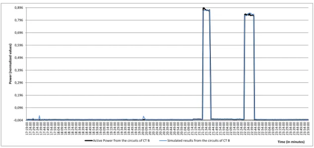
5.1 Simulation results versus the Active Power from circuits 2 and 4 from CT
B - all variables as inputs . . . 45
5.2 Error between the simulation results and the Active Power from circuits 2
and 4 from CT B - all variables as inputs . . . 45
5.3 Simulation results versus the Active Power from circuits 2 and 4 from CT
B - all variables as inputs (for 400 samples) . . . 46
5.4 Error between the simulation results and the Active Power from circuits 2
and 4 from CT B - all variables as inputs (for 400 samples) . . . 46
5.5 Simulation results versus the Active Power from circuits 5 and 7 from CT
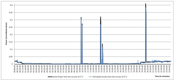
C - all variables as inputs . . . 47
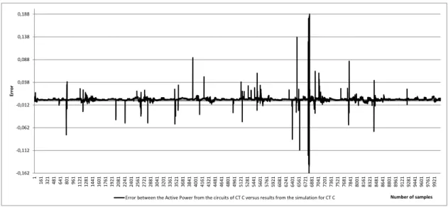
5.6 Error between the simulation results and the Active Power from circuits 5
and 7 from CT C - all variables as inputs . . . 47
5.7 Simulation results versus the Active Power from circuits 5 and 7 from CT
C - all variables as inputs (for 1440 samples) . . . 48
5.8 Error between the simulation results and the Active Power from circuits 5
and 7 from CT C - all variables as inputs . . . 48
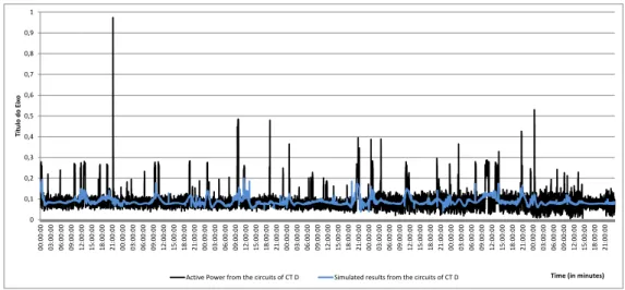
5.9 Simulation results versus the Active Power from circuits 8 and 9 from CT
LIST OF FIGURES xxi
5.10 Error between the simulation results and the Active Power from circuits 8
and 9 from CT D - all variables as inputs . . . 49
5.11 Simulation results versus the Active Power from circuits 2 and 4 from CT B - using the Active Power from the electrical switchboard as the only input 50 5.12 Error between the simulation results and the Active Power from circuits 2
and 4 from CT B - using the Active Power from the electrical switchboard
as the only input . . . 51
5.13 Simulation results versus the Active Power from circuits 2 and 4 from CT B - using the Active Power from the electrical switchboard as the only input
(for 450 samples) . . . 51
5.14 Error between the simulation results and the Active Power from circuits 2 and 4 from CT D - using the Active Power from the electrical switchboard
as the only input (for 450 samples) . . . 52
5.15 Simulation results versus the Active Power from circuits 5 and 7 from CT C - using the Active Power from the electrical switchboard as the only input 52 5.16 Error between the simulation results and the Active Power from circuits 5
and 7 from CT C - using the Active Power from the electrical switchboard
as the only input . . . 53
5.17 Simulation results versus the Active Power from circuits 5 and 7 from CT C - using the Active Power from the electrical switchboard as the only input
(for 850 samples) . . . 53
5.18 Error between the simulation results and the Active Power from circuits 5 and 7 from CT C - using the Active Power from the electrical switchboard
as the only input (for 850 samples) . . . 54
5.19 Simulation results versus the Active Power from circuits 8 and 9 from CT D - using the Active Power from the electrical switchboard as the only input 54 5.20 Error between the simulation results and the Active Power from circuits 8
and 9 from CT D - using the Active Power from the electrical switchboard
as the only input . . . 55
5.21 Simulation results versus the Active Power from circuits 2 and 4 from CT
B - using the date as the only input . . . 56
5.22 Error between the simulation results and the Active Power from circuits 2
and 4 from CT B - using the date as the only input . . . 56
5.23 Simulation results versus the Active Power from circuits 5 and 7 from CT
C - using the date as the only input . . . 57
5.24 Error between the simulation results and the Active Power from circuits 5
and 7 from CT C - using the date as the only input . . . 57
5.25 Simulation results versus the Active Power from circuits 8 and 9 from CT D 58 5.26 Error between the simulation results and the Active Power from circuits 8
xxii LIST OF FIGURES
A.1 Simulation results versus the Active Power from circuits 2 and 4 from CT
B - all variables as inputs . . . 74
A.2 Error between the simulation results and the Active Power from circuits 2
and 4 from CT B - all variables as inputs . . . 74
A.3 Simulation results versus the Active Power from circuits 5 and 7 from CT
C - all variables as inputs . . . 75
A.4 Error between the simulation results and the Active Power from circuits 5
and 7 from CT C - all variables as inputs . . . 75
A.5 Simulation results versus the Active Power from circuits 8 and 9 from CT
D - all variables as inputs . . . 76
A.6 Error between the simulation results and the Active Power from circuits 8
and 9 from CT D - all variables as inputs . . . 76
A.7 Simulation results versus the Active Power from circuits 2 and 4 from CT B - using the Active Power from the electrical switchboard as the only input 77 A.8 Error between the simulation results and the Active Power from circuits 2
and 4 from CT B - using the Active Power from the electrical switchboard
as the only input . . . 77
A.9 Simulation results versus the Active Power from circuits 5 and 7 from CT C - using the Active Power from the electrical switchboard as the only input 78 A.10 Error between the simulation results and the Active Power from circuits 5
and 7 from CT C - using the Active Power from the electrical switchboard
as the only input . . . 78
A.11 Simulation results versus the Active Power from circuits 8 and 9 from CT D - using the Active Power from the electrical switchboard as the only input 79 A.12 Error between the simulation results and the Active Power from circuits 8
and 9 from CT D - using the Active Power from the electrical switchboard
as the only input . . . 79
A.13 Simulation results versus the Active Power from circuits 2 and 4 from CT
B - using the date as the only input . . . 80
A.14 Error between the simulation results and the Active Power from circuits 2
and 4 from CT B - using the date as the only input . . . 80
A.15 Simulation results versus the Active Power from circuits 5 and 7 from CT
C - using the date as the only input . . . 81
A.16 Error between the simulation results and the Active Power from circuits 5
and 7 from CT C - using the date as the only input . . . 81
A.17 Simulation results versus the Active Power from circuits 8 and 9 from CT
D - using the date as the only input . . . 82
A.18 Error between the simulation results and the Active Power from circuits 8
List of Tables
3.1 Example of data stored and what each value represents . . . 31
3.2 Example of three samples of data stored . . . 31
3.3 Example of final data ready to be processed . . . 31
4.1 Correlation between the Active Power from the circuits of CTs B, C and D
and the different input variables . . . 36
5.1 Results for the simulation results versus the Active Power from circuits 2
and 4 of CT B - all variables as inputs . . . 44
5.2 Results for the simulation results versus the Active Power from circuits 5
and 7 of CT C - all variables as inputs . . . 47
5.3 Results for the simulation results versus the Active Power from circuits 8
and 9 of CT D - all variables as inputs . . . 48
5.4 Results for the simulation results versus the Active Power from circuits 2 and 4 of CT B - using the Active Power from the electrical switchboard as
input . . . 50
5.5 Results for the simulation results versus the Active Power from circuits 5 and 7 of CT C - using the Active Power from the electrical switchboard as
the only input . . . 52
5.6 Results for the simulation results versus the Active Power from circuits 8 and 9 of CT D - using the Active Power from the electrical switchboard as
the only input . . . 54
5.7 Results for the simulation results versus the Active Power from circuits 2
and 4 of CT B - using the date as the only input . . . 55
5.8 Results for the simulation results versus the Active Power from circuits 5
and 7 of CT C - using the date as the only input . . . 57
5.9 Results for the simulation results versus the Active Power from circuits 8
xxiv LIST OF TABLES
5.10 Comparison between the results obtained in section 5.1 for circuits 2 and 4
from CT B . . . 59
5.11 Comparison between the results obtained in section 5.1 for circuits 5 and 7
from CT B . . . 60
5.12 Comparison between the results obtained in section 5.1 for circuits 8 and 9
from CT D . . . 60
5.13 Comparison between results from 4 weeks worth of data and 8 weeks
worth of data - using all variables as inputs . . . 61
5.14 Comparison between results from 4 weeks worth of data and 8 weeks worth of data - using the Active Power from the electrical switchboard
entrance as the only input . . . 61
5.15 Comparison between results from 4 weeks worth of data and 8 weeks
Acronyms
AC Alternating Current
ANN Artificial Neural Networks
CFL Compact Fluorescent Light
CI Computational Intelligence
CT Current Transformers
EC Evolutionary Computing
FFT Fast Fourier Transform
HVAC Heating, Ventilation and Air Conditioning
I2C Inter-Integrated Circuit
LCD Liquid Crystal Display
NILM Non intrusive Load Monitoring
PSO Particle Swarm Optimization
RTC Real Time Clock
RMS Root Mean Square
SCL Serial Clock
SDA Serial Data
1
Introduction
1.1
Background and Motivation
Energy, as a whole, is a key element to modern civilization, and its consumption raises continuously due to several factors like the population growth or the increase of the stan-dards of life [1]. The energy consumption raises in such a continuous way, that predic-tions state that the energy demand will rise about 53% until the year 2030 [2]. This means that an increase in available energy is a necessity, which represents a problem because energy sectors world wide face serious problems when the topic is energy production, with the most commonly appointed solution being a sustainable energy development, mainly because this solution takes into account some of the most important factors, like the fight against climate changes, and also the increasingly scarce nature of fossil fuels [3, 4].
It’s mainly because of the on growing scarce nature of fossil fuels, and the impact of their applications on the environment, that governments worldwide are implementing energy saving measures, and so the need to implement new sources of energy increases [5, 6]. With this in mind, it’s important to tackle subjects like sustainable energy develop-ment, because its foundations are based on energy efficiency, and it’s widely agreed that energy efficiency is the most effective, and better way, to impact today’s environmental issues [3].
1. INTRODUCTION 1.2. Objectives
all the end-uses of energy, it’s easier to tackle energy efficiency in the end-use because ultimately changes in consumers behavior, whether industrial, commercial or domestic are easier to perform than to change entire systems already in place, because for instance, reducing the losses in the transformation processes is more of a technological problem (e.g. switching from fossil fuels to renewable energies, or improving the existing renew-able energy sources to better outputs) [3]. For instance, in studies like the one performed in [7], results showed that there is a lack of information with building users about how much energy is consumed by a building, or even by a specific electrical device, which is a big deal taking into account the fact that between 1997 and 2008, residential and in-dustrial buildings accounted for 56% of the European Union electrical consumption [8]. Nonetheless, it is easier to "educate" people, than to change entire systems that are already in place, as it was mentioned. Off course that changes in those two processes -educating people and changing/improving the systems that are already in place, is the ideal solution, but because technological setbacks prevents the enhancement of say for instance, a better usage and harnessing of renewable energies, it’s easier to provide solu-tions regarding energy efficiency on its end-use.
1.2
Objectives
With the objective of improving the energy efficiency in buildings, and to facilitate energy readings of those same buildings, this thesis has as its main objective the development of a module that, with the help of CI methods, has the ability to relate the Active Power of specific circuits from an electrical switchboard, to the total Active Power of that electrical switchboard.
In order to do this, the proposed solution is performed taking into account the fol-lowing steps:
• Development of a module - hardware and software - that has the ability to not only
collect data like the Active Power of a circuit, but that also has the ability to know at which time and day of the week the data is being collected;
• After the data is collected, there is a need to rearrange that data so it can be applied
to the chosen CI method;
• Once the data is rearranged, the chosen CI method is applied, along with
simula-tions to the results from the CI method applied, to see if a correlation between the total Active Power of an electrical switchboard and the Active Power of a circuit (or circuits) from that electrical switchboard can be established;
1. INTRODUCTION 1.3. Thesis Organization
1.3
Thesis Organization
Aside from this introductory chapter, this document is organized as follows:
Chapter 2:
In this chapter, an approach of the state of the art on subjects such as relevant fac-tors in energy consumption in buildings, energy auditing, Non intrusive Load Monitor-ing (NILM) systems, electricity monitorMonitor-ing systems and CI methods is performed.
Chapter 3:
In chapter 3, the proposed solution is presented as a whole. In other words, chap-ter 3 describes all that was necessary to develop the proposed module, as well as the CI method chosen.
Chapter 4:
Chapter 4 describes the implementation of the proposed solution. Most specifically, this chapter describes in detail the case study performed to validate the proposed solu-tion.
Chapter 5:
In this chapter, the obtained results are compared and discussed in detail.
Chapter 6:
2
State of The Art
This chapter has the purpose of reviewing a number of topics that are important to the developed work, such as relevant factors that influence energy consumption in buildings, energy audits, the analyses of similar products that can be found in markets, as well as several CI methods that can be applied to this specific work.
2.1
Relevant Factors in Energy Consumption in Buildings
Energy consumption in buildings depends on a number of factors, ranging from the weather conditions, to the direct consumption systems in the buildings (e.g. Heating, Ventilation and Air Conditioning (HVAC)), to the building’s characteristics (e.g. charac-teristics of the building’s structure), to the usage of the building itself (e.g. whether the building is commercial, residential, industrial or an office building), to the economical and environmental factors (e.g. electricity prices, environmental issues).
2.1.1 Economical Factors and Environmental Issues
2. STATE OFTHEART 2.1. Relevant Factors in Energy Consumption in Buildings
2.1.2 Building’s Characteristics
Another topic that influences energy consumption in buildings, is the building itself. In other words, the way the building is built, and also the materials used in it, affect energy consumption [11]. For instance, the better the heat storage capacity of an exterior wall of a building is, the less energy is going to be needed for heating because solar radiation can be stored during the day [12]. The building’s envelope also plays an important role in the energy consumption, because if the building’s envelope has an air leakage, people tend to raise or lower the temperature inside the building, depending on the time of the year. Another factor to be taken into account, is the fact of whether the building has a significant portion of its exposed surface covered by windows, in which case replacing the windows for more energy efficient windows (e.g. airtight, high-R value windows) has a significant effect on the building’s energy consumption [9, 13–15].
2.1.3 Building Usage
Whether the building is residential, commercial, industrial or an office, all of them are going to have different amounts of energy consumption, mainly because of what they’re meant to. It’s obvious that an industrial building is going to have a bigger energy con-sumption then a residential building for instance, mainly because industrial buildings have machinery/electrical devices that consume much more energy when compared to the typical electrical devices found in a household environment. It also becomes clear that the way in which people behave, is also going to have an impact on the building’s energy consumption. Whether it is the opening or closing of windows, lighting systems, or the personal regulation of HVAC systems, everything is going to have even the slightest im-pact on the energy consumption [16]. One example of human factors in energy consump-tion can be found in [17], where it was concluded that by automating the HVAC, shutters and lighting systems, savings of about 50% can be achieved. Because people’s behav-ior influences the building’s energy consumption, the amount of people in the building also has a direct effect on the energy consumption. A study was done in [18] regarding a building’s occupation, where it was concluded that the lifestyle of the occupants has an influence on the annual energy consumption of the building. For instance, the study shows that the fact that many office/factory workers aren’t home during the day leads to opposite energy profiles between offices/factories and homes. Because of this, factors like what kind of day it is (whether it’s a holiday, normal weekday or weekend) and also the time of the day are very important and must be taken into account.
2.1.4 Direct Consumption Systems
2. STATE OFTHEART 2.1. Relevant Factors in Energy Consumption in Buildings
consumption, typically assuming values in the range of 30-40% of a building’s consump-tion [20]. The energy consumpconsump-tion of HVAC systems is itself dependent of a number of factors where the most important one is the outside temperature [15, 19]. For instance
in [21] is shown that in Japan, when in peak demand period, a simple increase of 1oC
in temperature causes an increase of 4500 MW of energy demand. Because direct con-sumption systems depend on a large number of factors, they play a very important role in energy consumption, especially HVAC systems.
2.1.5 Weather Conditions
It is clear that the weather conditions have an impact on energy consumption [22]. Weather depends on a number of variables that have direct influence on energy consumption like [23]:
• Temperature;
• Solar light exposure;
• Rain;
• Wind velocity;
• Sky clearness;
Temperature: In a study conducted in [24], it was concluded that temperature is the
most important weather factor when it comes to energy consumption. Simply put, if it’s to hot, people tend to decrease the temperature inside the building. On the other hand, if it’s too cold, people tend to raise the temperature. This is done using HVAC systems, fans, oil heaters, etc, and this are all systems, as shown in the previous sections, that tend do have a high energy consumption ratio.
Solar light exposure: As discussed in section 2.1.2, buildings with walls that have
good heat storage capability, don’t need a lot of energy for heating or cooling the build-ing.
Rain:As shown in [25], rain can have a significant impact on relative humidity inside
buildings, thus creating the need to raise temperatures indoor.
Wind velocity: Wind has a direct impact on the temperature of the walls of a
2. STATE OFTHEART 2.2. Energy Auditing
Sky clearness: On a similar note, buildings that have systems with solar panels will
benefit from days that have clear skies versus days that are more clouded. Sky clearness also affects the solar light exposure that a building has, and ultimately will affect energy consumption as well.
Despite all the factors mentioned in this section, for this thesis, all the results pre-sented will only take into account the time of the day, and day of the week, because the case study done did not had the need, or in other words, did not justified the use of more variables, as it will be explained further on. Also, this two factors are very important in the sense that without the knowledge of what time it is, or what day of the week it is, there is no way to distinguish two points of equal power for instance.
2.2
Energy Auditing
Energy audit is a widely used term and may bare different meanings depending on the energy company that provides that service, but typically, four types of audits can be performed according to [9, 28]:
• Walk-through Audit;
• Utility Cost Analysis;
• Standard Energy Audit;
• Detailed Energy Audit;
Each of them will be briefly explained next.
2.2.1 Walk-through Audit
This type of audit consists on a simple and short on site visit of the facility being audited, in order to identify small and simple actions that provide immediate energy savings, like, for instance replacing broken windows, isolating exposed water/steam pipes or adjusting HVAC systems.
2.2.2 Utility Cost Analysis
2. STATE OFTHEART 2.2. Energy Auditing
important/dominant loads of the facility, because peak demand charges can be a signif-icant part of the electricity bill, and it can be concluded by the energy auditor that the facility can downscale or renegotiate the utility charges contract.
2.2.3 Standard Energy Audit
The standard energy audit, aside from performing all the steps as the two previous types of energy audits (see subsections 2.2.1 and 2.2.2), also provides a baseline for the en-ergy use of the facility, and also the evaluation of both the enen-ergy savings and cost-effectiveness of the energy conservation measures, through the use of simple tools like linear regression models. Also, typically a payback analysis is performed in order to determine the real cost-effectiveness of the the energy conservation measures applied.
2.2.4 Detailed Energy Audit
This type of energy audit is the most comprehensive one, but also the most time con-suming one. It includes the usage of measurement instruments to measure the energy consumption of the entire building, and/or of some energy systems inside the build-ing, more specifically end-use systems (direct consumption systems) such as lighting or HVAC systems. There are a number of techniques that allow energy measurements. For instance, during the on-site visit, clamp-on and/or hand-held equipment is used to de-termine variations of some of the building’s parameters, like indoor temperature, or en-ergy usage. These are the kind of parameters that are relatively easy to obtain. When more long-term measurements are required, usually sensors are used, that are connected to data-acquisition systems in order to store all the collected data, and also to have re-mote access to that data. In most recent years, energy auditors began to use the NILM technique (which will be explained further ahead). Because NILM techniques are asso-ciated with a minimal effort when compared to the traditional methods, they’re also a very attractive and inexpensive way to perform data-acquisition. In addition to the tech-niques mentioned above, sophisticated computer simulations are considered to evaluate and recommend energy savings for the building. The simulations performed by these computers provide the energy use by load type. A detailed energy audit also performs a more rigorous economic evaluation of the energy savings and cost-effectiveness mea-sures applied.
2. STATE OFTHEART 2.2. Energy Auditing
2.2.5 Energy Audit Example
This subsection aims to explore a case of an actual detailed energy audit made in [29]. The energy audit was done in a factory in Sri Lanka. The steps already described in sub-section 2.2.4 were performed, and in this case the aim of the energy audit was not only to specifically analyze and identify possible energy saving measures so that the monthly electrical bill would decrease, but also to help reduce production costs. Through the first steps of a detailed energy audit, it was possible to obtain the factory’s energy consump-tion, both in terms of functional area and also in terms of equipment consumption (see Figure 2.1 and Figure 2.2 showed next, respectively).
Figure 2.1: Area wise energy consumption, adapted from [29]
As expected, the production area has the highest values of energy consumption.
Figure 2.2: Equipment wise energy consumption, adapted from [29]
2. STATE OFTHEART 2.2. Energy Auditing
Next an evaluation was made in order to obtain the energy saving measures, and one of the points where it was found improvements could be made, despite not being the tems that showed highest energy consumption, was in the compressors and air dryer sys-tems by minimizing the air leakages, and through the installation of both variable speed controllers and intermittent controllers. Another set of improvements was made in the lighting systems by replacing incandescent lights by Compact Fluorescent Light (CFL), or by replacing the magnetic ballasts with electronic ones, among other replacements.
The conclusions made by this energy audit are very interesting, not only from the
point of view of cost reductions (seeing savings of around 3000e), but also from a more
personal point of view. For instance during the energy audit, the auditors found that em-ployee’s motivation was key to save energy without making serious investments. This can occur maybe because ultimately, all the measures proposed and implemented re-sult in the improvement of job security, as well as working and environment conditions. Lastly, it’s important to refer that all the measures suggested are of the entire responsibil-ity of the administration panel of the factory, and in this case, they decided to go through with them.
2.2.6 Energy Audit Application
This subsection explores a software application developed in [30], so that energy auditors have a practical methodology that is able to combine a predetermined set of principles and rules in energy auditing.
When using this software, users are able to add new cases, or open an existing case. There’s a tab for data collection showed in Figure 2.3.
2. STATE OFTHEART 2.2. Energy Auditing
In this tab, the user is capable of inserting for instance parameters regarding utility charges of the building, or a wide number of parameters about the building’s character-istics like the room’s length, width and height, wall colors, windows size, etc. The user is also able to insert other important parameters like the operating conditions of major en-ergy devices (HVAC for instance), average room temperature, among others. Summing up, this is where the user inserts all relevant information regarding the building’s energy consumption, as well as relevant information gathered during the on-site visit to the fa-cility being audited. The software is also able to provide suggestions for energy saving measures for each room audited, as shown in Figure 2.4.
Figure 2.4: Energy savings Tab [30]
It is important to refer that the energy savings measures shown on Figure 2.4 are merely demonstrative.
2. STATE OFTHEART 2.3. Non Intrusive Load Monitoring
2.3
Non Intrusive Load Monitoring
The first NILM system was developed by G. W. Hart in 1980. The origins of the first NILMs, or in other words, their purpose, was to monitor loads in residential buildings in order to get an insight about the final use of electricity [31–35]. Because G. W. Hart was "stuck" with the existing limitations of the computing power of that time, those sys-tems were initially designed to detect whether an appliance was plugged or unplugged (ON/OFF states) [32].
Basically, NILMs are systems that rely on external sensors or meters, which mea-sure Apparent, Reactive and Active Power. Those were the more rudimentary types of NILMs, or in other words, the first generation of NILMs. Next generation NILMs were the ones capable of processing the instantaneous voltage and current at the entry of where the energy is being measured [32].
For monitoring systems, it is possible to analyze measured data in steady state and in transient state [31, 33]. In the steady state analysis, individual load (or group of loads) are determined by analyzing and identifying the times where the electrical power mea-surement changes from a steady state value to another value [31]. In other words this type of method monitors the Active and Reactive Power, and then computes their differ-ences whenever a current variation occurs [33]. The transient state analysis relies on the behavior of the load to perform the load identification. In other words, the shape of the transient represents a specific class of loads, and then corresponds them to their electri-cal behavior. For a more efficient identification, this type of analysis compares each of the transient identified to a data base through the least squares criterion [31]. A simple diagram between this two types of states can be viewed in Figure 2.5.
Load Monitoring
Steady State
Transient State
Fundamental Fundamental + Harmonics
Admittance Current Power Spectral Analysis
Wavelet
Analysis HF
2. STATE OFTHEART 2.4. Electricity Monitoring Systems
2.4
Electricity Monitoring Systems
This subsection has the purpose of analyzing systems already in the market that are capa-ble of monitoring and provide feedback about electricity consumption. Research showed that a variety of these types of devices exist, from the ones that monitor a single device, to the ones capable of monitoring the energy consumption of an entire residence or a building, etc. The monitoring systems will be briefly reviewed next.
2.4.1 Socket Monitoring Systems
Kill a Watt P4400 and Power Monitoring for Dummies P4455:
On Figure 2.6 it’s possible to visualize two devices developed by P3 International that are socket monitoring systems [36]. The system shown in Figure 2.6(a) was the first device developed by P3 International. It is capable of tracking the overall power con-sumption of a device connected to it. It is also capable to check the quality of power by monitoring Voltage, Power Factor and line frequency. It has an additional interesting feature that is the ability to show the operating cost of the appliance connected to it with a 0,2% accuracy. The device shown on Figure 2.6(b) is an upgrade of the first one. Aside of having all the features of the first system, it is also capable of calculating the cumula-tive electrical expenses of the appliance connected to it and forecast usage by day, week,
month or year. These systems costs go for approximately 20eand 35erespectively.
(a) Kill a Watt P4400 [37]
(b) Power Monitor-ing For Dummies P4455 [38]
Figure 2.6: Examples of socket monitoring systems
2.4.2 Full "household" Monitoring Systems
2. STATE OFTHEART 2.4. Electricity Monitoring Systems
Wattson Solar Plus:
Figure 2.7: Wattson Solar Plus [39]
The Wattson Solar Plus [39], shown in Figure 2.7 is a system designed for residen-tial or small commercial buildings that have some kind of renewable energy system [39]. This system relies on sensors that are clamped on the electrical switchboard which in term transmit data to the Wattson panel shown on the Fig. 2.7. The clamps have to be put on the main feeder from the grid to the house (or small commercial building). If the house (or small commercial building) has any type of renewable energy system, a clamp can be put on the feeder that goes from the renewable energy system to the elec-trical switchboard. The system is capable of showing energy usage history, not only on the panel, but also on a computer, mobile phone or tablet. Perhaps the most interesting feature of this system is the colors display. For instance, when the panel shows the color green it means that there’s a surplus of energy. The system also knows how much of the surplus energy one can use, and so by knowing that there’s more energy being produced than energy being consumed, it is possible to increase savings and financial return. The panel is capable of showing three more colors, which are blue, meaning that energy con-sumption is below average, purple, which means that the energy being consumed is the normal/typical value of consumption for that building, and finally red, which means that the energy consumption is above the average use. The price for the Wattson Solar
Plus is approximately 195e.
2.4.3 Energy Meters and Energy Analyzers
Algodue UPT210 and UPM307 Energy Analyzers:
2. STATE OFTHEART 2.4. Electricity Monitoring Systems
(a) Algodue UPT210 Energy
Ana-lyzer [40] (b) Algodue UPM307 Energy An-alyzer [40]
Figure 2.8: Two different energy analyzers developed by Algodue
ports that provides the user means to connect it to a computer so data can be stored and then processed. The analyzer also has diagnostic capabilities like, for instance, the capability of detecting over/under-voltage or over-current which can indicate incorrect working conditions.
Figure 2.8(b) shows a more complex energy analyzer. Aside from having all of the capabilities of the Algodue UPT210, the Algodue UPM307 is capable of reading more than 100 electrical parameters. It also offers Fast Fourier Transform (FFT) analysis up to
the15thor
31thorder according to the accuracy. Among several more differences between
the two analyzers, the ones that standout more are maybe the fact that this analyzer is able to perform temperature readings, the fact that it possesses a high contrast graphic LCD, and also the fact that it provides the ability to download real-time waveform via communication ports.
Despite all the capabilities of this two analyzers, their prices are quite elevated, going
from approximately 155eto approximately 325erespectively [41].
It’s important to refer that this two analyzers are prepared to be integrated with CTs, like the ones shown on Figure 2.9.
(a) Hinged Split-Core Current
Transformer - 30A:333mV Ratio [42]
(b) Hinged Split-Core Current Transformer - 250A:333mV Ratio [43]
Figure 2.9: Two different types of current transformers developed by Ram Meter Inc
2. STATE OFTHEART 2.4. Electricity Monitoring Systems
analyses power, as some of these CTs are capable of grouping multiple feeding cables at a time, but they’re also very easy to install on an electrical switchboard. There is a large number of these type of CTs, going from rigid ones (like the ones on Figure 2.9) to
flexi-ble Rogowski coils for instance. Their price goes for approximately 20eto approximately
35e, respectively [42, 43], which are relatively cheap when compared to the prices of the
flexible Rogowski coils that go for approximately 140e[44].
Chauvin Arnoux Qualistar+ 8331:
The Chauvin Arnoux Qualistar+ 8331 [45] shown in Figure 2.10 is one of the most ad-vanced portable (and relatively compact) test and measurements instruments in the mar-ket nowadays. It is specifically designed for test and maintenance departments working in industrial and/or office buildings.
Figure 2.10: Chauvin Arnoux Qualistar+ 8331 [45]
It is extremely easy to handle and it offers a wide number of calculated values and processing functions. It is capable of performing all the features of the systems reviewed above, and then some more. It offers the possibility to connect current sensors to it, which it recognizes automatically and in term allows the direct reading of the measurements. Aside from being able to directly view the measurements done, the Chauvin Arnoux Qualistar+ 8331 allows the storage of those measurements, which can later be processed. This is possible because this device permits USB communication. With all its features, the Chauvin Arnoux Qualistar+ 8331 is the perfect tool to perform an energy audit.
With all it’s qualities aside, one major problem with this instrument is the way it has to be setup, because the voltage input terminals have to be connected to the circuit breakers, which is a somewhat delicate procedure. Another problem is its price, that is around
2. STATE OFTHEART 2.5. Computational Intelligence Methods
2.5
Computational Intelligence Methods
CI is a somewhat complex term, and over time has been interpreted in many different ways. Nonetheless, the most broad definition for CI according to [46] is that "CI is a branch of science studying problems for which there are no effective computational algo-rithms." These problems occur when trying to solve ill-defined vision tasks where formu-lating an exact and analytic algorithm is either impossible or computational wise, very demanding [47]. Another widely used definition of CI is: " CI is the study of adaptive mechanisms to enable or facilitate intelligent behavior in complex and changing envi-ronments. As such, CI combines ANN, Evolutionary Computing (EC), Swarm Intelli-gence (SI), and fuzzy systems." according to [48]. In the work developed in this thesis, the CI method used was the ANN, but nonetheless, it’s important to review some of the other existing CI methods.
2.5.1 Evolutionary Computing
EC is a research area within computer science. Its inspiration, as the name implies, comes from the process of natural evolution. So, according to [49], EC relates fundamentally to a particular style of problem solving, which is trial and error. Basically, EC is based on evolutionary algorithms, which has a very common idea behind it: survival of the fittest. In other words, when given for instance a quality function to be maximized, it is possible to create a random set of candidate solutions, i.e. elements of the functions domain, and then apply the quality function to determine a fitness measurement. Based on the results obtained when the quality function is applied (the higher the results, the better), the best candidates are selected to pass on to the next generation by applying recombination and/or mutation to them. Basically recombination is when an operator is applied to two or more candidates and that results in a new candidate, while mutation is when a change is made to a better candidate and that results in a new candidate. The new candidates "compete" and the process is repeated until a candidate considered fit enough is found, or until the computational limit is reached [49]. An example of an evolutionary algorithm can be seen in 2.11.
Current Population
Selection of Parents
Parent A Parent B
Recombination
Child A Child B
Mutation
Child A’
Child B’
New Candidates fit
enough? No
Yes Display
Results
2. STATE OFTHEART 2.5. Computational Intelligence Methods
2.5.2 Swarm Intelligence
SI derives from swarming behaviors of groups of organisms. This concept is interesting because it’s well known that group living enables problem solving that for a single indi-vidual are either very difficult or in some cases impossible. SI has the ability to manage very complex systems of multiple interacting individuals using minimal communication among them. They rely only on communications between local neighbors to produce a common, global behavior [50]. One of the most known types of SI is the Particle Swarm Optimization (PSO) method. It was inspired by swarming behaviors shown by flocks of birds. It has many resemblances with EC and the evolutionary algorithms, but it’s much faster and easier to implement a PSO method than an evolutionary algorithm because PSO does not have operators like mutation for instance [51]. Like the evolutionary algo-rithms in EC, PSO requires a fitness evaluation so the best solution can be assessed. Ba-sically PSO methods use computational entities that are distributed among the search/-work space, and in that space, each position represents a possible solution to the problem being analyzed. Each one of those computational entities is initialized in a random po-sition and with random velocity in the work space. With every increment of the system, the computational entities "travel" through the work space checking the fitness of each position that they traveled through, retaining information about the best location they visited. Because they’re capable of communicating with other computational entities, it is possible to compare the fitness of each location every computational entity visited, and then assess which one is the better one, so the swarm can converge upon that location, which represents the best possible solution among all the available solutions in that work space [50, 51].
2.5.3 Fuzzy Systems
2. STATE OFTHEART 2.5. Computational Intelligence Methods
is "very high", THEN the energy consumption of the building will be "somewhat high"".
2.5.4 Artificial Neural Networks
ANNs are mathematical models that take inspiration from biological neural networks. Their composition consists on artificial neurons, which in term take inspiration from nat-ural/biological neurons [55, 56].
Figure 2.12: Biological neuron [55]
Figure 2.12 shows a representation of a biological neuron. These neurons receive signals through synapses located on the membranes, or dendrites of the neuron (the dendrites are the "little branches" of the neuron). When the received signals are strong enough the neuron is activated and in term emits a signal through the axon. Those signals can be sent to another synapse which then repeats this process.
∑
Activation functionX
X
X
X
X
X
X
X
1
2
3
n
W
W
1
2
W
3W
nINPUTS
OUTPUT
Bias
2. STATE OFTHEART 2.5. Computational Intelligence Methods
Figure 2.13 represents an artificial neuron. In this case, the information comes to the
neuron in the form of inputs (X1 to Xn). These inputs are then multiplied by weights
(represented byW1 to Wn) and are then summed along with a bias. These values are
then processed by the activation function, which generates an output. A mathematical description of an artificial neuron can be viewed on Equation 2.1 [56].
Y(k) =F(
m X
i=0
Wi(k)×Xi(k) +b) (2.1)
To breakdown Equation 2.1,Xi(k)is the input value in discrete timekwhereigoes
from0tom. Wi(k)is the weight, also in discrete timek, whereialso goes from0tom.
The variablebisbias. F is the transfer (or activation) function. And finally,Y(k)is the
output value in discrete timek[56].
As it was mentioned before, signals processed by a neuron (biological or artificial) can be sent to another neuron. It’s when two or more neurons are combined that ANNs are obtained. To better understand ANNs, the artificial neurons are displayed in lay-ers. This type of architecture is called Perceptron and it can be singlelayer or multilayer accordingly to how many layers the ANN has. Figure 2.14 shows an example of an ANN.
Input
Layer
Hidden
Layer
Output
Layer
IN
P
U
T
V
A
LUES
Out
put
V
a
lue
s
X
1X
2X
3X
4X
5W
11W
12W
33W
15W
35Y
1Y
2W
11W
23W
12Figure 2.14: Simple representation of an Artificial Neural Network
2. STATE OFTHEART 2.5. Computational Intelligence Methods
training, the learning process is a function between the difference of the output of the ANN and the wanted value, and so, the weights keep changing until that difference is considered acceptable. When the training is unsupervised the ANN "evolves" for itself until it reaches an equilibrium point. This two types of training methods are used by the feedforward algorithm, as well as the backpropagation algorithm, which will be briefly explained next.
Feedforward
This type of process, or algorithm, is the simpler one, because it has only one con-dition: all the information must go forward, from input to output, with no back-loops [56]. Basically, with the feedforward algorithm, the input layer passes the activation of the artificial neuron to the next layer, and so on, until the output layer is reached.
Backpropagation
The backpropagation algorithm is somewhat more complex than the feedforward al-gorithm, because backpropagation algorithms are used in layered feedforward ANNs [55]. Firstly this algorithm uses supervised learning, which in other words means that examples of the input and output data that is going to be processed are provided for the ANN to compute. From this "computation" an error is calculated (this error is the dif-ference between the actual and the expected results). With this being said, initially back-propagation algorithms function in the exact same way as the feedforward algorithm, meaning that information flows forward from input to output. When the information reaches the output layer, the calculated errors of that information are propagated back-wards [55].
All the CI methods presented here are valid solutions for an enormous number of problems. However, a great number of studies shows that the most commonly used method when dealing with energy consumption, energy loads, etc, is the ANN [57, 58]. In some cases, studies have shown that fuzzy logic and ANN are indeed two of the methods that have the best results when compared to other methods [59].
3
Proposed Solution
What is proposed in this thesis is the development of a module - hardware and software - that provides the ability to relate the Active Power of previously selected circuits from an electrical switchboard, to the total Active Power of that electrical switchboard, as Fig. 3.1 shows.
Electrical
Switchboard
Module
Total
S
S
S
n2 1
Figure 3.1: Global view of the proposed solution
3. PROPOSEDSOLUTION 3.1. EmonTx Shield V1
The module shown in Fig. 3.1 is divided in the components shown in Fig. 3.2.
Data
Acquisition
System
Clock
Data Storage
Sensors
Figure 3.2: Overview of the developed module
The data acquisition system is composed by an EmonTx Shield V1 along with the Arduino Mega 2560, both shown in Fig.3.3.
(a) EmonTx Shield V1 [60] (b) Arduino Mega 2560 [61]
Figure 3.3: Hardware solution - EmonTx Shield V1 and Arduino Mega 2560
The reason behind the choice of this two items is because regarding the EmonTx Shield V1, this hardware provides the capability to monitor electricity, temperature, elec-trical current (RMS value) as well as Apparent Power, and its price is relatively low when
compared to the devices shown in section 2.4, costing approximately 15e. Because the
EmonTx Shield V1 requires a "base station" to send/receive data to/from, the choice landed on the Arduino Mega 2560. This was the arduino chosen among all the others, because this arduino has all the communication pins separated, which as it will be shown
further ahead, is a major concern with this setup. The price for this arduino is about 40e.
3.1
EmonTx Shield V1
3. PROPOSEDSOLUTION 3.2. Arduino Mega 2560
one shown in Fig. 3.4(a).
All that it’s left to know now is the Active Power, and in order to do that, parameters like the Power Factor and AC RMS voltage are needed. To obtain this last set of param-eters, a voltage sensor (which also serves as a power plug for the system) like the one shown in Fig. 3.4(b) is required.
(a) 100A max clip-on current sensor CT [62] (b) AC voltage sensor [63]
Figure 3.4: Hardware solution - chosen CT and AC voltage sensor
This two sensors represent the sensors shown in Fig. 3.2. It’s important to refer that
the price range of this two pieces is of approximately 12e for both the CT and the AC
voltage sensor.
With the setup so far, the system is capable of providing one of the parameters that is intended, which is the Active Power of a circuit to where the CT is connected. But as it was mentioned above, it is also required to know which time it is, the day of the week, and to be able to store all the data obtained. This points will be explained in the next section, for they are obtained through a few devices that need to be connected to the Arduino Mega 2560.
3.2
Arduino Mega 2560
As it was mentioned above, this was the "base station" chosen for the EmonTx Shield V1. The main reason behind this is because this arduino has its communication pins all separated. This is important because the EmonTx Shield V1 uses, among all the others, the pins 4 and 5 to send data to the "base station" (the arduino in this case). This wouldn’t be a problem if it wasn’t necessary to obtain parameters like the time or the day of the week, which in this case is done through a module (add-on) like the one shown on Fig. 3.5.
3. PROPOSEDSOLUTION 3.2. Arduino Mega 2560
Figure 3.5: DS3231 AT24C32 Memory Module For Arduino I2C Real Time Clock
and it represents the clock as its shown on Fig. 3.2. What this module does, as the name indicates, is that it provides the time and also the date. It possesses a special feature that is a battery casing, for when the system is not powered up, the battery keeps the RTC running and so the time is always updated. The problem, or conflict between the RTC and the EmonTx Shield V1, is the fact that in most arduinos, the pins 4 and 5 are also the Serial Data (SDA) and Serial Clock (SCL) pins, which preform the Inter-Integrated Circuit (I2C) communications between the RTC and the arduino. This represents a conflict because the arduino can’t receive data from the EmonTx Shield V1 and from the RTC at the same time. Plus, because the communication from the EmonTx Shield V1 to the arduino is not made using I2C, the system sometimes reads the data from the RTC, and sometimes reads the data sent from the EmonTx Shield V1. Because of this, the simpler solution for this problem was to choose the Arduino Mega 2560, which as it was already mentioned, has all the communications pins separated.
The final piece for the setup to be completed, is a module, like the one shown in Fig. 3.6, that is able to store all the data being collected, whether it’s the data from the EmonTx Shield V1, or the data from the RTC. It is important to refer that this module requires an actual SD card to store the data.
3. PROPOSEDSOLUTION 3.3. Complete System Assembled
Both the RTC and the SD Card Breakout Module can be acquire at relatively low
prices, of about 1eeach.
3.3
Complete System Assembled
Once all the components come together, the final module - hardware wise - is obtained, as shown on Fig. 3.7.
Figure 3.7: Final system
On Fig. 3.7 is possible to see:
• A - EmonTx Shield V1;
• B - Arduino Mega 2560;
• C - DS3231 AT24C32 Memory Module For Arduino I2C RTC;
• D - SD Card Breakout Module;
![Figure 2.5: Comparison between steady state and transient analyses, adapted from [31]](https://thumb-eu.123doks.com/thumbv2/123dok_br/16567276.737855/39.892.164.783.754.1092/figure-comparison-steady-state-transient-analyses-adapted.webp)