VIDENCE FROM THE EMU

M

ASTER OF

S

CIENCE IN

M

ONETARY AND

F

INANCIAL

E

CONOMICS

M

ASTERS

F

INAL

W

ORK

D

ISSERTATION

M

ONETARY

D

EVELOPMENTS AND

E

XPANSIONARY

F

ISCAL

C

ONSOLIDATIONS

:

E

VIDENCE FROM THE

EMU

L

UÍS

P

EDRO

M

ARQUES

M

ARTINS

M

ASTER OF

S

CIENCE IN

M

ONETARY AND

F

INANCIAL

E

CONOMICS

M

ASTERS

F

INAL

W

ORK

D

ISSERTATION

M

ONETARY

D

EVELOPMENTS AND

E

XPANSIONARY

F

ISCAL

C

ONSOLIDATIONS

:

E

VIDENCE FROM THE

EMU

L

UÍS

P

EDRO

M

ARQUES

M

ARTINS

S

:

A

A

Acknowledgements

I would like to thank Professor António Afonso, for outstanding support. It has been a

privilege.

Also, I would like to express my deepest appreciation to my parents. This dissertation

is dedicated to them.

Contents

1. Introduction ... 6

2. Motivating expansionary fiscal consolidations ... 8

2.1. Theoretical framework ... 8

2.2. Literature survey ... 10

3. Identification of fiscal and monetary episodes in the EMU ... 13

3.1. Fiscal episodes ... 13

3.2. Monetary episodes ... 15

4. Empirical assessment ... 18

4.1. Data description ... 18

4.2. Modelling expansionary fiscal consolidations ... 19

4.2.1. Core specification outputs ... 20

4.2.2. Fiscal consolidations and monetary expansions. ... 22

4.3. Measuring the success of fiscal consolidations ... 26

5. Conclusions ... 33

Appendix ... 35

References ... 47

Table I - Identification of the fiscal episodes according to the different criteria ... 14

Table II – Identification of the monetary episodes according to the different criteria (1970-2012) ... 17

Table III – Descriptive statistics ... 18

Table IV – Fixed Effects estimation results for specification (2) ... 21

Table V – Fixed Effects estimation for specification (3): 1st output ... 23

Table VI – Fixed Effects estimation for specification (3): 1st output (cont.) ... 24

Table VII – Fiscal consolidation events and success rates ... 27

Table VIII – Expenditure and revenue based consolidations: λ=2/3 ... 28

Table IX – Success of fiscal consolidations for 1 SU based on 2 FC ... 31

Table X - Success of fiscal consolidations for 2 SU based on 1 FC ... 32

Table XI – Data sources ... 35

Table XII – Descriptive statistics of the variables used to identify the fiscal and monetary episodes ... 35

Table XIII – Unit root tests for the series used in the fixed effects estimations ... 36

Table XIV - Descriptive statistics for the series used in the probit estimations ... 36

Table XV – Fixed Effects estimation for specification (3): 2nd output ... 37

Table XVI – Fixed Effects estimation for specification (3): 2nd output (cont.) ... 38

Table XVII – Fixed Effects estimation for specification (3): 3rd output ... 39

Table XVIII – Fixed Effects estimation for specification (3): 3rd output (cont.) ... 40

Table XIX – Wald coefficient diagnostics for estimations based on specification (3) ... 41

Table XX – Successful fiscal consolidations according to the different criteria (1970-2012) 42 Table XXI – Expenditure and revenue based consolidations: λ=1/2 ... 42

Table XXII – Expenditure and revenue based consolidations: λ=3/4 ... 43

Table XXIII – Success of fiscal consolidations forSU1 based on FC1 ... 43

Table XXIV – Success of fiscal consolidations forSU1 based on FC3 ... 44

Table XXV – Success of fiscal consolidations forSU2 based on FC2 ... 45

Table XXVI – Success of fiscal consolidations forSU2 based on FC3 ... 46

Abstract

This paper provides new insights about the existence of expansionary effects during fiscal

consolidations in the Economic and Monetary Union, using annual panel data for 14

European Union countries over the period 1970-2012. Different measures for assessing fiscal

consolidations based on the changes in the cyclically adjusted primary balance were

calculated. A similar ad-hoc approach was used to compute monetary expansions in order to

include them in the assessment of non-Keynesian effects for different budgetary components.

Panel fixed effects estimations for private consumption show that, in some cases, when fiscal

consolidations are coupled with monetary expansions, the traditional Keynesian signals are

reversed for general government final consumption expenditure, social transfers and taxes.

Keynesian effects prevail when fiscal consolidations are not matched by a monetary easing.

Panel probit estimations suggest that longer and expenditure based consolidations contribute

positively for its success, while the opposite holds for the tax based ones.

1. Introduction

Keynesian theory gives us some insights about the expected effect of government

budgetary components’ changes on income. It postulates that an increase in government

spending should stimulate the economy, via the multiplier mechanism, thus increasing

disposable income and private consumption. Based on this reasoning, an increase in taxation

should lead to a decrease in private consumption.

Nevertheless, since the early 90’s, having studied the case studies of Denmark and

Ireland1, some literature has been discussing the possible non-Keynesian effects of fiscal

policy, namely during fiscal consolidation periods.

The theoretical underpinnings stemmed from the German Council of Economic

experts in their reports of 1981 and 1982, and are referred to as the “expectational view of

fiscal policy”.2 Arguably, the standard Keynesian relationship between private consumption

and government budgetary components may be reversed under certain circumstances. A

deterioration of the fiscal position (resulting in a budget deficit) today may lead to an increase

in taxation in the future in order to comply with the government budget constraint, therefore

reducing the agents’ permanent income. If such expectations are accepted by individuals, then

this could lead to a decrease in private consumption today. The reverse reasoning holds for a

fiscal consolidation, meaning that an improvement in the fiscal position may lead to an

increase in private consumption today. Some empirical research presents evidence that

supports this view.3

The expectational view of fiscal policy relies on the assumption of Ricardian

households, which have a smoothing effect on consumption and do not have liquidity

constraints. This motivates a thorough assessment of the monetary developments when

expansionary fiscal consolidations are being studied. Moreover, according to the Keynesian

view, under the IS-LM framework, a fiscal consolidation may lead to an increase in private

consumption if accompanied by a strong enough monetary expansion that offsets the

detrimental effects of fiscal policy developments on disposable income and private

consumption.

1 _{See Giavazzi & Pagano (1990).} 2 _{See Hellwig & Newmann (1987).}

3

See for instance, Giavazzi & Pagano (1990), Perroti (1999), Ardagna (2004), Afonso (2006, 2010) and Alesina & Ardagna (2013).

Arguably, while neglecting the monetary policy stance, one could find themselves in a

situation described by Ardagna (2004): “In this case, the coefficients of fiscal policy variables

can be biased, capturing the effect of monetary rather than fiscal policy”.

The importance of this issue within the Economic and Monetary Union (EMU) context

is fairly obvious, since the expectational view of fiscal policy was to some extent reflected in

the fiscal convergence criteria of the Maastricht Treaty. Additionally, the monetary policy

stance is outside the national governments’ sphere of influence.

This paper contributes to the existing literature by providing some new insights about

the importance of the monetary stance for the relationship between fiscal developments and

private consumption during fiscal consolidation periods. It does so by expanding notably

Afonso’s (2006, 2010) and Afonso & Jalles’s (2014) core specification in order to

accommodate the monetary policy developments. I conduct an assessment of the fiscal

episodes using the same criteria. However, and in addition, I also identify monetary episodes

for 14 European Union countries from 1970 to 2012 and study their relationship with fiscal

developments.

This paper contributes to existing literature by providing some new insights about the

importance of the monetary stance for the relationship between fiscal developments and

private consumption during fiscal consolidation periods. It does so by notably expanding

Afonso’s (2006, 2010) and Afonso & Jalles’s (2014) core specification, in order to take into

account monetary policy developments. We conduct an assessment of the fiscal episodes,

using the same criteria. However, and in addition, we also identify monetary episodes for 14

European Union countries from 1970 to 2012, and study their relationship with fiscal

developments.

The paper is organised as follows. Section two presents the review of the main related

literature. Section three presents an identification of the fiscal and monetary episodes and

their respective relationship. In section four, we conduct an empirical analysis of

expansionary fiscal consolidations for the EMU, resorting to panel estimations, taking into

account the developments of monetary policy, followed by a discussion of the results. We

also assess, relying on a probit estimation, the factors that may impinge on the success of the

fiscal consolidations, namely expenditure based versus revenue based consolidations, using

the fiscal and monetary episodes identified in the earlier sections. Section five concludes with

some final remarks and points out some possible subjects for future research on this topic.

2. Motivating expansionary fiscal consolidations

2.1. Theoretical framework

According to Prammer (2004), the effects of a fiscal consolidation may be

traditionally viewed under a Keynesian, Ricardian or Neoclassical framework.

The standard Keynesian view, suggests that a fiscal contraction has downturn effects

on aggregate demand, economic activity and employment, at least in the short-run. These

downturns can occur directly, through cuts in government expenditure, thus reducing

aggregate demand, or indirectly, through tax increases which reduce disposable income,

dampening private consumption. Given the usual multipliers, cuts in public spending should

lead to more severe downturns than an increase on taxation.

Nevertheless, according to the Keynesian arguments, a fiscal consolidation can be

expansionary if accompanied by a sufficiently expansionary monetary policy, which

highlights the possible role of the monetary policy in the outcomes of expansionary fiscal

consolidation episodes.

The Ricardian equivalence theorem challenges this view: an increase in public

spending (resulting in a budget deficit) shouldn’t lead to an increase in private consumption,

since in order to satisfy the intertemporal budget constraint, the deficit must be offset by an

increase in taxation in the future. Therefore, it is equivalent to tax financing and can’t lead to

an increase in aggregate demand. Barro (1974) further develops this issue, within a rational

expectations framework. Rational agents are aware that in order for governments to pay the

cost of financing budget deficits today, they must increase taxes in the future. Therefore a

fiscal stimulus shouldn’t lead to an increase in private consumption, but higher savings

instead.

The Neoclassical outcome of fiscal stimulus on economic growth is similar to the one

in Ricardian equivalence, although it operates through a different channel. Rational agents

optimize their consumption over their lifecycle. In this context it is possible to shift the tax

burden caused by budgets deficits to the next generations and therefore private consumption

may increase, contrary to the Ricardian equivalence proposition. Nevertheless, as private

consumption increases, so do the interest rates, due to lower savings, leading to a decrease in

private investment, thus offsetting possible positive effects of private consumption on growth.

This Neoclassical line of thought is summarized in Afonso (2006): “According to

Neoclassical theory, a budget reduction would have no effect on economic activity since the

supply side is supposed to be the main determinant of economic growth”.

The hypothesis of non-Keynesian effects of a fiscal consolidation stemmed from the

German Council of Economic experts in their 1981 and 1982 reports, as seen in Hellwig &

Newman (1987).

A key point is the “expectational view of fiscal policy” which states that a fiscal

consolidation that is seen as credible and long lasting can signal future taxation ease, thus

inducing a wealth effect. Future lower taxes increase households’ permanent income. Since

consumers expect to be wealthier in the future, they will smooth their consumption by

increasing it today. As pointed out by Alesina & Ardagna (1998), the size of the increase in

private consumption depends on the absence of liquidity-constrained consumers.

On the demand side, the credibility of fiscal consolidations affects interest rates.

Lower government debt should reduce the risk premium and the real interest rate of

government debt. It also should stimulate private investment, through reduced cost of

financing spill-over effects. A risk premium is likely to be higher when the debt-to-GDP ratio

crosses some threshold, since there is a higher debt service burden and default gets a real

possibility. Therefore, non-Keynesian effects should be more likely for fiscal consolidations

when the levels of government debt are high.

This reasoning is explored in Blanchard (1990) and Sutherland (1997)’s models in

which high levels of debt can lead to non-linear consumer behaviour. The amount of tax

increase when the level of public debt is high generates significant deadweight loss. In this

sense, a fiscal consolidation today reduces the probability of sharp tax increases in the future,

thus inducing a wealth effect due to a decrease in expected deadweight loss. Arguably, in this

context, the positive wealth effect is stronger than the negative impact of increased taxation

today on private consumption. The same is not true for lower levels of debt-to-GDP ratio

since the tax burden could fall on the future generations, so consumers have no expectation of

facing significant deadweight loss, meaning that the wealth effect will be weaker than the tax

increase effect on private consumption.

This also relates to Bertola & Drazen (1993)’s consumption optimizing behaviour

model in which upward trends in government spending increase the probability of a fiscal

consolidation, since a stabilization program might be necessary at specific “trigger points” to

ensure the sustainability of public finances. These fiscal consolidation moments induce an

expectation of future tax cuts, thus increasing permanent income.

On the supply side, Alesina & Ardagna (1998) argue that wage moderation may

contribute to the likelihood of an expansionary fiscal consolidation event. If union’s demands

for wage increase (following an increase in labour taxes) are met, this will result in loss of

competitiveness due to higher labour costs. Therefore, an agreement on wage moderation with

the unions may foster or at least may not have a detrimental effect on investment and growth

following a fiscal consolidation episode.

2.2. Literature survey

Hellwig & Neumann (1987) were pioneers with regard to the postulation of the

expansionary fiscal consolidation hypothesis. They argue that fiscal consolidation in Germany

in the 1980’s under Chancellor Kohl had such a positive impact on private sector confidence

that demand actually increased. Supposedly, fiscal consolidation by the Federal Government

and monetary tightness by the Bundesbank led to continued growth of output and low

inflation. Also lower deficits stimulated private investment in the long run, due to reduced

cost of financing. Nevertheless, unemployment remained high, which authors attribute to

labour market rigidity.

Giavazzi & Pagano (1990) test this hypothesis for Denmark and Ireland for the mid

and late 1980's, respectively. For Denmark, they report that the thriving consumption

experienced in 1983-1986 cannot be explained by the decline in interest rates alone, and that

such an occurrence is related to fiscal consolidation through the increase in revenue from

income taxation and the decrease in public investment. Regarding the Irish case, the fast

growth of consumption during the second stabilization was due to the government’s focus on

decreasing spending, instead of increasing taxation, and also due to the liberalisation of the

credit markets. In these cases, as a whole, expansionary fiscal consolidation is linked to an

adjustment on the side of public spending, rather than on revenues, although in Denmark, the

adjustment was through investment spending and in Ireland, it was through current spending.

Alesina & Ardagna (1998) investigate the expansionary fiscal consolidation

possibility, using an analysis of OECD countries from 1960 to 1994. According to the

General Council of Economic Experts’ expectational view of fiscal policy addressed in

Hellwig and Neumann (1987), fiscal adjustments that occur when the debt level is high, or

growing rapidly, should be expansionary, whereas others should not. Nevertheless the authors

don’t find evidence that confirms this view. On the other hand, they found strong evidence of

the effect of the composition of the adjustment in the outcome of fiscal consolidation: all of

the non-expansionary adjustments were tax-based and all of the expansionary ones were

based on expenditure cuts. Expenditure adjustments that were accompanied by wage

moderation and by nominal exchange rate devaluation, turned out to be expansionary.

Perroti (1999) addresses the same issue for nineteen OECD countries from 1965 to

1994, and, according to his findings, substantial deficit cuts can lead to booms in private

consumption. The likelihood of an expansionary fiscal consolidation increases in times of

“fiscal stress”, which the author defines as periods of high debt-to-GDP ratio or following

periods of exceptionally high debt-accumulation rates. His findings differ for other periods, as

in “normal” times, the Keynesian effects of fiscal consolidation on private consumption

predominate (either through spending cuts, or tax increases).

Giavazzi et al. (2000) address the issue of expansionary fiscal consolidation in OECD

countries from 1973 to 1996 and in developing countries from 1960 to 1995. In OECD

countries evidence of non-Keynesian response by the private sector is more likely to be found

when the fiscal impulses are large and persistent. This means that only those can signal a

regime change, thus affecting private sector expectations. Also non-Keynesian effects leading

to an expansionary fiscal consolidation are stronger for changes in net taxes rather than in

public expenditure. In developing countries, non-Keynesian effects occur not only during

periods of fiscal contractions but also during fiscal expansions and when countries are piling

up debt rapidly, regardless of its level.

Using panel data from OECD countries from 1970 to 2002, Ardagna (2004)

investigates the effect of fiscal consolidations on debt-to-GDP ratio and GDP growth.

Regarding debt-to-GDP ratio, the success of fiscal consolidation depends more on the size of

the adjustment, rather than its composition. On the other hand, the likelihood of fiscal

consolidation being expansionary, increases when it is based on public spending cuts, rather

than on increased taxation. Concerning the role of monetary policy, there was evidence that

neither successful (leading to decrease in debt-to-GDP ratio), or expansionary (leading to

increase in GDP growth) consolidations, need to be met by expansionary monetary policies,

nor by exchange rate devaluations.

Giudice et al. (2004) address the matter of non-Keynesian effects in fourteen

European Union countries, in an ex-post and ex-ante analysis. Ex-post analysis consisted on

studying the period from 1970 to 2002 to see whether fiscal consolidation episodes were

followed by an increase in GDP growth. Results show that this occurred in about half the

cases. The ex-ante analysis carried out was based on simulations by the European

Commission QUEST model and suggested that short-term non-Keynesian effects can occur, if

consolidation is mainly on the spending side. The latter is also true in the ex-post case, which

is in line with most empirical studies.

Afonso (2006, 2010) conducted a panel analysis for 15 EU countries from 1970 to

2005, having found some evidence of non-Keynesian effects in private consumption for some

government spending items, namely final consumption and social transfers. Results show that

a decrease in government consumption leads to an increase in private consumption in the long

run, and the magnitude of this effect is higher when a fiscal consolidation episode occurs.

Devries et al. (2011) construct a database for fiscal consolidation measures taken by

17 OECD countries from 1978 to 2009, based on the premise that computing fiscal

consolidations from changes of the cyclically adjusted primary balance may be problematic.

Arguably, such an approach may be biased, in the sense that it may capture changes that are

not related to policy actions due to its inability to remove sharp fluctuations in economic

activity. Therefore, they identify fiscal consolidations through an historical approach, based

on policy documents. This database has been widely used in subsequent literature that

concerns expansionary fiscal consolidations.4

Afonso & Jalles (2012) analyse a panel of OECD countries from 1970 to 2010, to

assess whether the composition and duration of fiscal consolidations contribute to their

success. Consolidation episodes lead to a decrease in debt ratios, only if they are accompanied

by strong economic growth and an increased output gap. Increased duration contributes to the

success of the fiscal consolidation episode. Fiscal consolidation success depends on the

composition of the adjustment: consolidations based mainly on tax increases, contribute

negatively to its success.

Alesina & Ardagna (2013) use a Devries et al. (2011) policy action-based approach to

identify the fiscal episodes for 21 OECD countries from 1970 to 2010. They conclude that

expenditure based adjustments are more likely to be successful and expansionary. Monetary

policy is not significant for explaining the differences between expenditure-based and

tax-based adjustments.

To sum up, most of the research seems to support, or at least not to reject, the idea of

expansionary fiscal episodes.5 Also, some findings6 suggest that expansionary and successful

fiscal episodes are more likely when there is consolidation on the spending side.

Moreover, some of the literature, such as Perroti (1999) and Giavazzi et al. (2000).

propose that non-Keynesian effects are more likely to, or only occur, during periods of high

debt-to-GDP ratio or when debt is accumulating quickly.

4 _{See, for instance, Afonso & Jalles (2012) and Alesina & Ardagna (2013).}

5 _{As seen in Giavazzi & Pagano (1990), Alesina & Ardagna (1998), Perroti (1999), Giavazzi et al. (2000), van}

Aarle & Garretsen (2003), Ardagna (2004), Giudice et al. (2004) and Afonso (2006, 2010).

6 _{Giavazzi & Pagano (1990), Alesina & Ardagna (1998), Afonso (2006, 2010) and Alesina & Ardagana (2013).}

3. Identification of fiscal and monetary episodes in the EMU

3.1. Fiscal episodes

Most of the empirical literature relies on the change in the cyclically adjusted primary

balance (CAPB) as a percentage of GDP, as measure of governments’ structural budget

balance. It extracts those elements of the primary balance that are due to the business cycle,

from the total balance, in order to obtain an indicator that has been corrected for the effects of

changes in economic activity, and that thus reflects the discretionary part of the fiscal policy.

Table XI in the Appendix shows some descriptive statistics of this indicator.

One can assess the existence of fiscal episodes – either contractions or expansions – by

studying the behaviour of this indicator over time. In Giavazzi & Pagano (1996), a fiscal

episode occurs when the cumulative change in the cyclically adjusted primary balance is at

least 5, 4, or 3 percentage points of GDP in 4, 3 or 2 years respectively, or 3 percentage points

in one year. Alesina & Ardagna (1998) identify the periods of occurrence of fiscal episodes

by looking for the periods when the change in the cyclically adjusted primary balance was

greater than 2 percentage points in one year, or at least 1.5 percentage points of GDP on

average in the last two years. Afonso’s (2006, 2010) assessment of fiscal episodes relies on a

different method: a fiscal episode occurs when the change in the cyclically adjusted primary

balance is greater than 1.5 times the panel standard deviation of this indicator, or when the

average absolute change in the last two years is greater than the standard deviation of the full

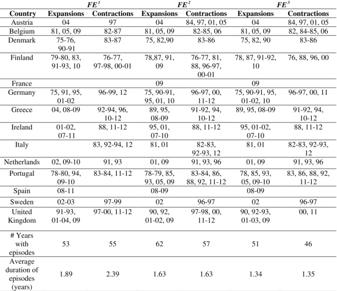
panel. Table I shows the fiscal expansions and contractions according to the different criteria.7

The measures used by Giavazzi & Pagano (1996), Alesina & Ardagna (1998) and

Afonso (2006, 2010), were labelled respectively as 1

FE , 2

FE and 3

FE . Overall, there is a

considerable overlapping of episodes according to the different criteria:- there is a

coincidence of 82 and 63 percent between fiscal episodes 1 and 2 and 1 and 3, respectively

and 82 percent between criteria 2 and 3 (see Table I).

All the criteria reflect the cases studied by Giavazzi and Pagano (1990), as fiscal

contractions in Denmark in 1983-86 and in Ireland in 1988 were identified. Also, there is a

clear identification of fiscal expansions in 2009 across the EMU countries, which followed

the European Commission policy recommendations after the 2007-08 financial crisis. The

different methodologies also identify the consolidation efforts made by those countries that

were subject to financial assistance in 2010-2012, namely Ireland, Greece and Portugal.

7 _{We used a slightly lower threshold for the Afonso (2006, 2010) methodology, due to the increase in the}

standard deviation of the panel sample from 1.57 to 2.00. We used 1, instead of 1.5 times the standard deviation.

Table I - Identification of the fiscal episodes according to the different criteria (1970-2012) 1 FE 2 FE 3 FE

Country Expansions Contractions Expansions Contractions Expansions Contractions

Austria 04 97 04 84, 97, 01, 05 04 84, 97, 01, 05 Belgium 81, 05, 09 82-87 81, 05, 09 82-85, 06 81, 05, 09 82, 84-85, 06 Denmark 75-76,

90-91

83-87 75, 82,90 83-86 75, 82, 90 83-86

Finland 79-80, 83, 91-93, 10 76-77, 97-98, 00-01 78,87, 91, 09 76-77, 81, 88, 96-97, 00-01

78, 87, 91-92, 10

76, 88, 96, 00

France 09 09

Germany 75, 91, 95, 01-02

96-99, 12 75, 90-91, 95, 01, 10

96-97, 00, 11-12

75, 90-91, 95, 01-02, 10

96-97, 00, 11

Greece 04, 08-09 92-94, 96, 10-12

89, 95, 08-09

91-92, 94, 10-12

89, 95, 08-09 91-92, 94, 10-12 Ireland 01-02,

07-11

88, 11-12 95, 01, 07-10

88, 11-12 95, 01-02, 07-10

88, 11-12

Italy 83, 92-94, 12 81, 01 82-83, 92-93, 12

81, 01 82-83, 92-93, 12 Netherlands 02, 09-10 91, 93 01, 09 91, 93, 96 01, 09 91, 93, 96

Portugal 78-80, 94, 09-10

83-84, 11-12 78-79, 85, 93, 05, 09

83-84, 86, 88, 92, 11-12

78, 85, 93, 05, 09-10

83, 86, 88, 92, 11-12

Spain 08-11 08-09 08-09

Sweden 02-03 97-99 02 96-97 02 96-97

United Kingdom

91-93, 01-04, 09

97-00, 11-12 90, 92, 01-02, 09 97-98, 00, 11-12 90, 92-93, 01-03, 09 00, 11 # Years with episodes

53 55 62 57 51 46

Average duration of

episodes (years)

1.89 2.39 1.63 1.63 1.34 1.35

Recent studies, such as Afonso & Jalles (2012) and Alesina & Ardagna (2013), also

include a criterion for identifying fiscal consolidations referred to as IMF’s “Action Based

Approach”, which was computed by Devries et al. (2011). It identifies fiscal consolidations

based, not on the changes in CAPB, but on an historical approach through the analysis of

policy documents. Arguably CAPB-based fiscal consolidations may be biased, in the sense

that they may capture changes that are not related to policy actions due to their inability to

remove sharp fluctuations in economic activity. Unfortunately, the database is still not

up-to-date so we would have to discard the most recent years (2010-2012) in order to use that

approach. Therefore, we will not include it at this point, but we intend to do so in future

research.

Source: author’s computations. Notes: FE1- Measure based on Giavazzi & Pagano (1996); FE2- Measure

based on Alesina & Ardagna (1998); FE3- Measure based on Afonso (2006, 2010).

3.2.Monetary episodes

One of the main points in this paper is the study of the coupling of fiscal and monetary

policy, in order to assess whether monetary expansions have an impact on the relationship

between government budgetary components and private consumption during fiscal

consolidation episodes. Therefore, it is crucial to establish a clear identification of the

monetary episodes in the EMU countries. We chose three indicators that could be used as a

measure of the monetary stance for the different countries, namely: the real short term money

market interest rate, and the nominal and real effective exchange rates.

The change in the real short term interest rate is a widely used measure of monetary

policy easing or tightening8, as it accounts not only for money market rates, but also for price

developments. Therefore, a negative variation in this indicator signals a real monetary easing,

rather than a nominal one.9

Both the nominal and the real effective exchange rate assess the currency value in a

country vis-à-vis a weighted average of other selected countries’ currencies, which is

commonly used to assess a country’s competitiveness. The nominal effective exchange rate

has been used by Ardagna (2004) as an indicator of the monetary stance. A negative change

in this indicator corresponds to currency depreciation and therefore monetary expansion. We

also included the real effective exchange rate, with the purpose of accounting for possible

differences in monetary episodes-identification due to price developments, which links to the

arguments presented about the interest rates case.

In order to define monetary episodes, we relied on a similar strategy as Afonso (2006,

2010) and identified an episode when the absolute change in one year, or the average change

in two years, in the different indicators was greater than 1.5 times, or 1 times the panel

standard deviation respectively:

1

1, 1, 5

1, 1, 2, 3

2 0,

l l

t

l l

l t t l

t

if M

M M

ME if l

otherwise σ

σ

−

 ∆ > 

 _{∆ + ∆}

=_ > =

  

. (1)

8 _{See, for instance, Afonso & Sousa (2011).}

9 _{Since nominal short-term interest rates are very similar in the EMU countries from 1999 onwards, we cannot}

include them in our estimations, due to near singular matrix issues and therefore they were excluded from this analysis.

l t

ME denotes a monetary episode in period t, according to criterion l and l t

M

∆

corresponds to the change of indicator l in period t. For real short term interest rate, we have

an absolute change, whilst for the nominal and real effective exchange rates, we used the

percentage change of the respective indexes. 𝜎𝑙 stands for the panel standard deviation of the relevant indicator.

Table II shows the monetary episodes identified according to the different indicators.

1

ME , 2

ME and 3

ME correspond to the use of the methodology across the changes in the real

short term interest rate, and the percent changes in the real and nominal effective exchange

rate, respectively.

One of the main findings, is that there are considerably more monetary episodes than

fiscal ones. The duration of monetary episodes also changes significantly across the different

criteria. If we look at the monetary episodes based on the change in the real short term interest

rate ( 1

ME ), it is possible to see that the expansions and contractions last 1.5 and 1.8 years on

average, respectively. If we consider the changes in the nominal effective exchange rates, then

the duration of expansions more than doubles, and in the case of contractions, it also increases

significantly.

Moreover, while in the case of fiscal episodes, there is significant overlapping across

the different criteria, in this case it is much lower, with the matching being only 38, 51 and 63

percent between 1

ME and 2

ME , 1

ME and 3

ME and 2

ME and 3

ME , respectively. The

splitting between expansions and contractions is fairly even, with the exception of 3

ME ,

which registered considerably more contractions than expansions. Also, we can see that there

are episodes labelled as expansions in ME1 that show up as contractions in ME2 andME3, which further motivates the inclusion and analysis of all the different criteria.10

The descriptive statistics of the indicators used to identify both fiscal and monetary

episodes can be consulted in table XII in the Appendix.

10 _{For instance, in Austria, monetary expansion in 1983 expansion is shown according toME}1_{, but it shows up as}

a contraction in_ME3_.

Table II – Identification of the monetary episodes according to the different criteria (1970-2012) 1 ME 2 ME 3 ME

Country Expansions Contractions Expansions Contractions Expansions Contractions

Austria 72, 83, 94, 09-10

77, 80-81, 89-90

97-98, 00 77, 80, 87, 93, 95, 04

73-80, 83, 86-88, 93, 95 Belgium 72,75,

82-83, 93-94, 10 76-77, 79-81, 90-91 81-83, 97-98, 00

77, 79, 86-87, 95, 03-04

81-83, 97 77-78, 86-87, 91, 95,

03-04 Denmark 73, 81,

94-97, 10

76-78, 90-91, 93, 07, 11

80-82, 00 79, 86-87, 03-04, 09

80-82, 00 73-74, 76, 86-87, 90-91, 93, 95,

03-04 Finland 71-74, 88,

93-95, 98, 12 75-76, 80, 83-84, 89-92 72, 78-79, 92-94, 97, 00, 11 74-76, 80-82, 85, 89-90, 95-96, 03-04 72-73, 78-79, 92-93, 97, 00 81, 89-90, 94-96, 03-04

France 72, 75-76, 94, 97

74, 77, 81, 90 82-84, 97-98, 00-01

86-87, 03-04 77-78, 81-84, 00

73, 75-76, 86-87, 90, 93-96,

03-04 Germany 75, 82-83,

86, 93, 02, 09-10

73, 80-81, 90 81-82, 85, 89, 97-98, 00-01, 11

79, 87, 93-95, 03-04

97, 00 72-80, 83-84, 86-88, 93-96,

03-04 Greece 82, 90,

95-96, 00-03

86, 89, 92-94, 98

83-86, 00-01

82, 88, 90-91, 95-96, 03-04,

08

72-95 03-04

Ireland 75-76, 81, 88-89, 92-94, 98-99, 10-12 74, 77-79, 83-85, 90-91, 07-09 88-89, 93-94, 99-00, 10-12 79-80, 82-83, 86-87, 02-04, 07-08 73-77, 81-82, 84, 99-00 86, 90-91, 03-04, 08

Italy 73-74, 94, 99, 09

76, 81-85, 92 93-95, 00 83-84, 86-87, 90-91, 96-97, 03-04 73-85, 93-95, 00 87, 96-97, 03-04

Netherlands 71-72, 94-95, 10

73-74, 78-80, 90, 07

81, 84-85, 89, 97, 00

77, 79, 87, 95, 02-04

97 74-78, 83, 86-88, 93-95 Portugal 73-75, 80,

83, 88, 94-95, 98, 10

76-79, 81-82, 85, 87, 90-91,

08 77-80, 83-84 81-82, 89-93, 02-04 76-89, 94

Spain 84-86, 88, 95, 99 78-81, 83, 87-88, 07-08 82-84, 93-94 85-91, 02-03, 08 76-78, 81-84, 93-94 74, 79, 89-91, 03-04 Sweden 86-87,

93-94

85, 92-93 78, 82-84, 93-94, 98-02, 09 79-80, 85, 89-91, 96, 03-04, 10-12 78-79, 82-84, 93-94, 01-02, 09

76, 96-97, 03-04, 10-12 United Kingdom 74-75, 88, 02, 09-10 73, 76-77, 81-82, 90, 98

83-84, 86-87, 93-94, 08-10

80-81, 88-89, 91, 97-99, 05, 07, 11-12 73-77, 83-84, 87, 93-94, 08-10 79-81, 88, 97-99 # Years with episodes

96 92 95 124 124 122

Average duration of

episodes (years)

1.55 1.80 1.98 1.85 3.26 2.22

Source: author’s computations. Notes: ME1- Measure based on the changes in the real short term interest rate;

2

ME - Measure based on changes in the real effective exchange rate; _ME3_{- Measure based on the changes in}

4. Empirical assessment

4.1. Data description

The data consists on an annual frequency time series ranging from 1970 to 2012 for

private consumption, GDP, general government final consumption, social transfers, taxes,

cyclically adjusted primary balance, general government debt, revenue and expenditure, that

was taken from the AMECO database.11 We used 11 countries that belong to the EMU,12

namely Austria, Belgium, Germany, Finland, France, Greece, Ireland, Italy, The Netherlands,

Portugal and Spain and also Denmark, Sweden and The United Kingdom, which are not in the

EMU, but are geographically and politically linked to the remaining countries. This means

that a maximum of 602 observations are available per variable, throughout the entire panel.

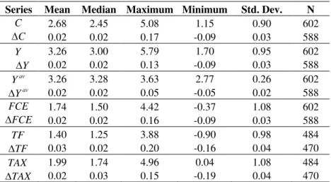
Table III shows the descriptive statistics for the series used in the estimations

presented in section 4.2.

Table III – Descriptive statistics

Series Mean Median Maximum Minimum Std. Dev. N

C 2.68 2.45 5.08 1.15 0.90 602

C

∆ 0.02 0.02 0.17 -0.09 0.03 588 Y 3.26 3.00 5.79 1.70 0.95 602

Y

∆ 0.02 0.02 0.13 -0.09 0.03 588

av

Y 3.26 3.28 3.63 2.77 0.26 602

av

Y

∆ 0.02 0.02 0.05 -0.05 0.02 588

FCE 1.74 1.50 4.42 -0.37 1.08 602

FCE

∆ 0.02 0.02 0.16 -0.09 0.03 588 TF 1.40 1.25 3.88 -0.90 0.98 484

TF

∆ 0.03 0.02 0.20 -0.16 0.04 470 TAX 1.99 1.74 4.96 0.04 1.08 484

TAX

∆ 0.02 0.03 0.15 -0.19 0.04 470

All variables are displayed as the logarithm of the real per capita observations. We

can see that there is no missing data for private consumption (C), GDP (Y), panel average

GDP ( av

Y ) and general government final consumption expenditure (FCE) throughout the

entire panel, since that we have the maximum number of possible observations (602). Even

so, the general government budgetary components such as social transfers (TF) and taxes

(TAX) series have some missing data.

The unit root tests in table XIII in the Appendix show that most series are stationary.

For the ones that are not, since I have already computed significant changes on the original

11 _{For full description of the original series, see table X in the Appendix.}

12 _{Originally we also had Luxembourg, which was dropped, due to the lack of information on monetary data.}

Source: author’s computations.

series, such that what we have are the logarithms of the real per capita values, it makes sense

to include all the series in levels. Otherwise we would risk losing some of the intuition behind

the variable relationship, thus making the model more difficult to interpret.13

Table XIV in the Appendix shows the descriptive statistics of the variables used in the

probit estimations in section 4.3.

4.2. Modelling expansionary fiscal consolidations

The strategy for accessing the potential differences between fiscal expansions and

fiscal contractions is based on Afonso (2006, 2010). It consists on estimating the variation of

private consumption, using budgetary variables and dummies for assessing fiscal and

monetary episodes. The core specification will be:

1 0 1 1 0 1 1

1 1 3 1 1 3 1 1 3

2 1 4 2 1 4 2 1 4

( )

( ) (1 )

av av

it i it it it it it

m

it it it it it it it

m

it it it it it it it it

C c C Y Y Y Y

FCE FCE TF TF TAX TAX FC

FCE FCE TF TF TAX TAX FC

λ ω ω δ δ

α α β β γ γ

α α β β γ γ µ

− − −

− − −

− − −

∆ = + + + ∆ + + ∆ +

+ ∆ + + ∆ + + ∆ × +

+ ∆ + + ∆ + + ∆ × − +

(2)

where (i i=1,..., )N indicates the different countries, (t t=1,..., )T stands for the period. We

also have: C– private consumption; Y – GDP; av

Y – panel’s GDP average;14 FCE – general

government final consumption expenditure; TF – social transfers; TAX – taxes. All variables

displayed correspond to the natural logarithm of the real per capita values.15 m

FC is a

dummy variable that identifies a fiscal consolidation episode, according to the three different

criteria mentioned in the previous section (m=1, 2,3). Therefore, when m it

FC is equal to one,

there is a fiscal consolidation in period t, for country i, according to the criterion m.ciis an

autonomous term which captures each country’s individual characteristics, being the source of

cross-country heterogeneity in a Fixed Effects model, which will be our estimation choice.

The disturbances µit are assumed to be independent and identically distributed across

countries with zero mean and constant variance.

13 _{My argument follows the explanation presented in Afonso (2006, 2010).}

14 _{The original specification in Afonso (2006, 2010) used the OECD’s GDP instead of the panel average.}

Nevertheless, since OECD only displays that series starting from 1995 I followed Afonso & Jalles (2011) and used the panel average GDP.

15 _{For instance, in order to obtain the variable Y , we make the following calculations:} /

ln GDP DEF Y

N

 

= _ _, where GDP stands for the GDP at current prices, DEF and N correspond to the GDP deflator and total population, respectively.

4.2.1. Core specification outputs

According to Greene (2012), we use the Fixed Effects (FE) estimation whenever we want

to analyse the impact of variables that change over time. This explores the relationship

between predictor and dependent variables within a country. The FE model removes the effect

of time-invariant characteristics from the predictor variables, so that we can assess the

independent variables net effect. An important assumption of the model is that time invariant

characteristics are country-specific, and should not be correlated with other individual

features. In other words, each country has unique attributes that are not the result of random

variation and do not vary across time. The source of country heterogeneity is provided by the

intercept ci in specification (1), with Fixed Effects allowing for correlation between the latter

and the repressors.16

We perform redundant FE likelihood ratio tests for all estimations, with the null

hypothesis being that there is no unobserved heterogeneity and so the model can be estimated

by pooled OLS. If we reject this hypothesis, then fixed effects is more adequate than pooled

OLS, since it allows for cross country heterogeneity by permitting each one to have its own

intercept value (ci).

17

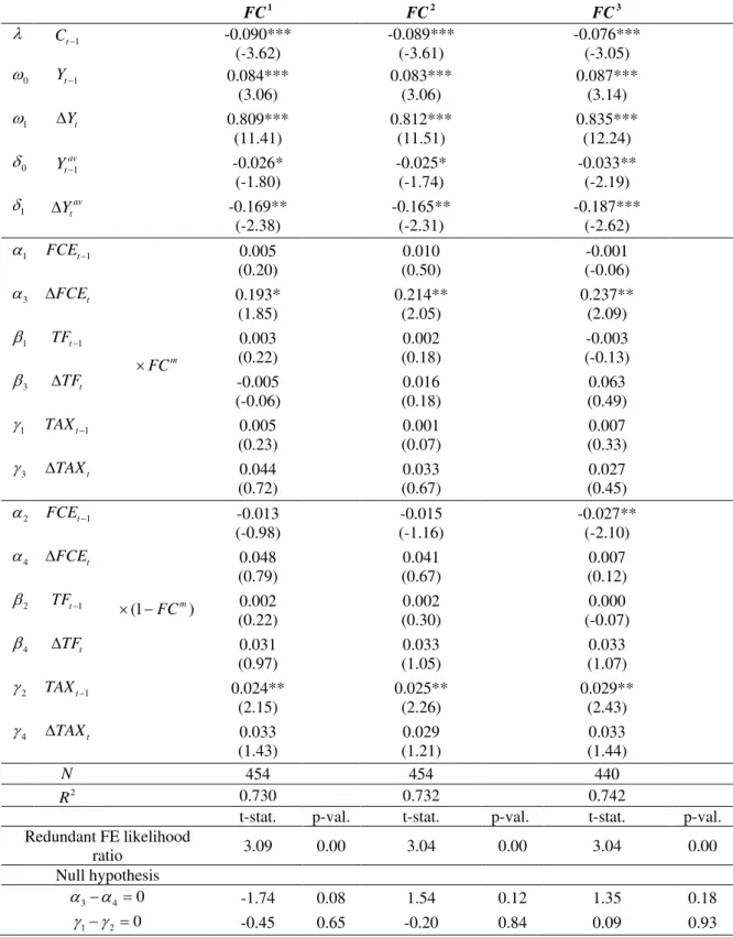
Table IV presents the estimation results for specification (2), according to the different

criteria for identifying fiscal consolidation episodes. Both consumption and income are

statistically significant across the different specifications. The negative sign for consumption

in t-1 (λ) has obviously to do with the fact that lagged consumption has been considered an

independent variable, therefore increasing consumption in period t-1 reduces its difference

between t and t-1. The short-run elasticity of private consumption to income is similar across

specifications, ranging between 0.083 and 0.087.

16 _{In the FE estimation, the intercept also works as a substitute for non-specified variables, yielding consistent}

estimates in the presence of correlation between the latter and the repressors, which favours the usage of this model in comparison to pooled OLS.

17 _{We report the redundant FE likelihood ratio for all estimations. In any case, the no cross-country heterogeneity}

assumption is always rejected, which means that the FE estimator is more adequate than pooled OLS.

Table IV – Fixed Effects estimation results for specification (2)

1

FC _FC2 _FC3

λ C_t−1 -0.090***

(-3.62) -0.089*** (-3.61) -0.076*** (-3.05) 0

ω Y_t−1 0.084***

(3.06) 0.083*** (3.06) 0.087*** (3.14) 1

ω ∆Y_{t 0.809***}

(11.41) 0.812*** (11.51) 0.835*** (12.24) 0

δ av₁ t

Y− -0.026*

(-1.80) -0.025* (-1.74) -0.033** (-2.19) 1 δ av t Y ∆ -0.169** (-2.38) -0.165** (-2.31) -0.187*** (-2.62) 1

α FCEt−₁

m FC × 0.005 (0.20) 0.010 (0.50) -0.001 (-0.06) 3

α ∆FCE_t 0.193*

(1.85) 0.214** (2.05) 0.237** (2.09) 1

β TF_t−1 0.003

(0.22) 0.002 (0.18) -0.003 (-0.13) 3

β ∆TFt -0.005

(-0.06) 0.016 (0.18) 0.063 (0.49) 1

γ TAX_t−1 0.005

(0.23) 0.001 (0.07) 0.007 (0.33) 3

γ ∆TAX_t 0.044

(0.72) 0.033 (0.67) 0.027 (0.45) 2

α FCE_t−1

(1 m)

FC × − -0.013 (-0.98) -0.015 (-1.16) -0.027** (-2.10) 4

α ∆FCE_t 0.048

(0.79) 0.041 (0.67) 0.007 (0.12) 2

β TF_{t−1 0.002}

(0.22) 0.002 (0.30) 0.000 (-0.07) 4

β ∆TF_t 0.031

(0.97) 0.033 (1.05) 0.033 (1.07) 2

γ TAX_t−1 0.024**

(2.15) 0.025** (2.26) 0.029** (2.43) 4

γ ∆TAX_{t 0.033}

(1.43)

0.029 (1.21)

0.033 (1.44)

N 454 454 440

2

R 0.730 0.732 0.742

t-stat. p-val. t-stat. p-val. t-stat. p-val. Redundant FE likelihood

ratio 3.09 0.00 3.04 0.00 3.04 0.00

Null hypothesis

3 4 0

α α− = -1.74 0.08 1.54 0.12 1.35 0.18

1 2 0

γ γ− = -0.45 0.65 -0.20 0.84 0.09 0.93

Notes: Used robust heteroskedastic-consistent standard errors. The t-statistics are in parentheses. *, ** and

*** denotes statistically significant at a 10, 5 and 1 percent level, respectively. 1

FC - Measure based on

Giavazzi & Pagano (1996); 2

FC - Measure based on Alesina & Ardagna (1998); 3

FC - Measure based on

Afonso (2006, 2010).

There is a positive statistically significant relationship between the first difference of

general government final consumption expenditure (∆FCEt) and private consumption (∆Ct),

when a fiscal consolidation ( m =

FC 1) occurs, across all of the estimations based on (2), with

coefficients between 0.193 and 0.237. Such a relationship is in line with the traditional

Keynesian effects, indicating that consumers are not behaving in a Ricardian way, since they

do not seem to anticipate the need for increased taxation in the future, to compensate for an

increase in government spending today.

The previous relationship does not hold in the absence of a fiscal consolidation

episode. Moreover, there is some evidence of non-Keynesian effects in the absence of fiscal

consolidations ( m =

FC 0), if we look at the final consumption expenditure (FCEt 1− ) and

taxes (TAXt 1₋ ) in column 3, and across the three different estimations, respectively. The

negative sign in the short-run elasticity of general government final consumption expenditure

to private consumption suggests a Ricardian behaviour, in the absence of fiscal

consolidations. Similar non-Keynesian reasoning prevails for the relationship between taxes

and consumption, meaning that an increase in taxes today, leads to increased spending, as

consumers anticipate that there is no need for increased taxation in the future.

However, the Wald coefficient statistical tests suggest that there is no significant

difference between the presence or absence of fiscal consolidations in relation to the short-run

effects of government final consumption expenditure and taxation on private consumption

(the null hypothesis: α α₃− ₄ =0and γ γ₁− ₂ =0 are not rejected on the third, and all specifications, respectively).

Compared with the literature that used similar methodology, as a whole, our results

differ from Afonso (2006, 2010) and Afonso & Jalles (2012), since we find no evidence of

non-Keynesian effects with regards to general government final consumption expenditure or

taxes in the presence of fiscal consolidations ( m =

FC 1). However, our findings are similar

for periods of no fiscal consolidation ( m =

FC 0), as there is some evidence of non-Keynesian

effects in this case, for the mentioned budgetary variables.

4.2.2. Fiscal consolidations and monetary expansions.

The following specification is one of the main contributions of this paper, adding each

country’s monetary developments to specification (2). It will permit a breakdown of all the

possible combinations between fiscal contractions and monetary expansions, thus allowing

for the study of the possible differences between them:

1 0 1 1 0 1 1

10 1 30 10 1 30 10 1 30 50

20 1 40 20 1 40 20 1 40 60

( )

(

av av

it i it it it it it

l m l

it it it it it it it it it

it it it it it it i

C c C Y Y Y Y

FCE FCE TF TF TAX TAX M FC MX

FCE FCE TF TF TAX TAX M

λ ω ω δ δ

α α β β γ γ η

α α β β γ γ η

− − − − − − − − − ∆ = + + + ∆ + + ∆ + + ∆ + + ∆ + + ∆ + ∆ × + + ∆ + + ∆ + + ∆ + ∆

11 1 31 11 1 31 11 1 31 51

21 1 41 21 1 41 21 1 41 61

) (1 )

( ) (1 )

( ) (1 )(1 )

l m l

t it it

l m l

it it it it it it it it it

l m l

it it it it it it it it it it

FC MX

FCE FCE TF TF TAX TAX M FC MX

FCE FCE TF TF TAX TAX M FC MX

α α β β γ γ η

α α β β γ γ η µ

− − − − − − × − + + ∆ + + ∆ + + ∆ + ∆ × − + + ∆ + + ∆ + + ∆ + ∆ × − − + (3)

In addition to the repressors previously explained, l it

MX denotes a monetary expansion in

period t (t=1,..., )T for country i (i=1,..., )N according to the criteria l(l=1, 2,3). l

M ∆

corresponds to the relevant indicator used to calculate the monetary episodes on (1). We have

found some evidence of non-Keynesian effects during fiscal consolidations in 5 out of the 9

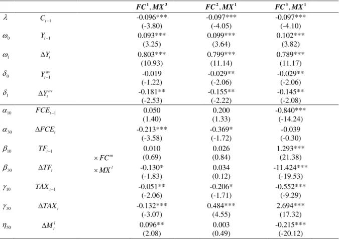
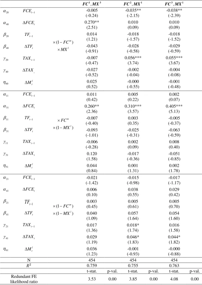
possible estimations.18 Tables V and VI show some of the most relevant estimation results.

Table V – Fixed Effects estimation for specification (3): 1st output

,

1 3

FC MX _FC2_,MX1 _FC3_,MX1

λ C_t−1 -0.096***

(-3.80) -0.097*** (-4.05) -0.097*** (-4.10) 0

ω Y_t−1 0.093***

(3.25) 0.099*** (3.64) 0.102*** (3.82) 1

ω ∆Y_t 0.803***

(10.93) 0.799*** (11.14) 0.789*** (11.17) 0

δ av₁ t

Y₋ -0.019

(-1.22) -0.029** (-2.06) -0.029** (-2.06) 1 δ av t Y ∆ -0.181** (-2.53) -0.155** (-2.22) -0.145** (-2.08) 10

α FCE_t−1

m FC × l MX × 0.050 (1.40) 0.200 (1.33) -0.840*** (-14.24) 30

α ∆FCE_t -0.213***

(-3.58) -0.369* (-1.72) -0.039 (-0.30) 10

β TF_t−1 0.010

(0.69) 0.026 (0.84) 1.293*** (21.38) 30

β ∆TF_t -0.130*

(-1.83) 0.034 (0.12) -11.424*** (-19.53) 10

γ TAX_t−1 -0.051**

(-2.06) -0.206* (-1.71) -0.552*** (-9.29) 30

γ ∆TAX_t -0.132***

(-3.07) 0.484*** (4.55) 2.694*** (17.32) 50 η l t M ∆ 0.096** (2.08) 0.003 (0.49) -0.215*** (-20.12)

18 _{Notice that since we have three different criteria for fiscal and monetary developments, the assessment of their}

relationship within the current framework yields 9 possible estimation outputs. The other outputs are available in tables XV-XVIII in the Appendix.

Table VI – Fixed Effects estimation for specification (3): 1st output (cont.)

,

1 3

FC MX _FC2_,MX1 _FC3_,MX1

20

α FCE_t−1

(1 m)

FC × − l MX × -0.005 (-0.24) -0.035** (-2.15) -0.038** (-2.39) 40

α ∆FCE_t 0.270**

(2.51) 0.010 (0.09) 0.010 (0.09) 20

β TFt−₁ 0.014

(1.21) -0.018 (-1.57) -0.018 (-1.52) 40

β ∆TF_t -0.043

(-0.91) -0.028 (-0.58) -0.029 (-0.59) 20

γ TAX_t−1 -0.007

(-0.47) 0.056*** (3.74) 0.055*** (3.67) 40 γ t TAX ∆ -0.027 (-0.52) -0.002 (-0.04) -0.004 (-0.08) 60 η l t M ∆ 0.025 (0.52) -0.000 (-0.55) -0.001 (-0.48) 11

α FCE_t−1

m FC

× (1 l)

MX × − 0.011 (0.42) 0.005 (0.22) 0.002 (0.07) 31

α ∆FCE_t 0.260**

(2.36) 0.310*** (3.57) 0.405*** (5.13) 11

β TF_t−1 -0.007

(-0.40) 0.003 (0.35) -0.005 (-0.37) 31

β ∆TFt -0.093

(-1.01) -0.025 (-0.31) -0.063 (-0.59) 11

γ TAX_t−1 -0.006

(-0.28) 0.002 (0.09) 0.008 (0.40) 31

γ ∆TAX_t 0.120

(1.58) -0.017 (-0.36) -0.051 (-0.85) 51 η l t M ∆ 0.044 (0.84) 0.001 (1.31) 0.002 (1.78) 21

α FCE_t−1

(1 m)

FC

× − (1 l)

MX × − -0.021 (-1.42) -0.015 (-0.98) -0.017 (-1.17) 41

α ∆FCE_{t 0.006}

(0.10) 0.038 (0.55) 0.029 (0.42) 21 β 1 t

TF₋ 0.003

(0.45) 0.005 (0.61) 0.005 (0.70) 41

β ∆TF_t 0.040

(1.09) 0.057 (1.64) 0.054 (1.60) 21

γ TAX_t−1 0.017

(1.36) 0.018* (1.74) 0.016 (1.58) 41

γ ∆TAXt 0.029

(1.19) 0.046* (1.83) 0.044* (1.82) 61 η l t M ∆ 0.036 (1.23) -0.001 (-0.93) -0.000 (-0.88)

N 454 454 454

𝑅2 _{0.759 0.755 0.763}

t-stat. p-val. t-stat. p-val. t-stat. p-val. Redundant FE

likelihood ratio 3.53 0.00 3.85 0.00 4.08 0.00

Notes: Used robust heteroskedastic-consistent standard errors. The t-statistics are in parentheses. *, ** and

*** denotes statistically significant at a 10, 5 and 1 percent level, respectively.

We can see that when fiscal consolidations are matched by monetary expansion, there is a

negative and statistically significant short-term elasticity between the government final

consumption expenditure and private consumption (α₃₀ <0 in the first and second outputs and α₁₀ <0 in the third output). This doesn’t hold when fiscal consolidations that are not accompanied by a monetary easing as α₃₁is positive and statistically significant, and α₁₁is not statistically significant across the respective outputs. The second and third estimation results

also show some evidence of non-Keynesian elasticity on taxes, when there are both fiscal

contractions and monetary expansions (γ₃₀ >0). Just like in previous cases, such effects seem to disappear when fiscal consolidations take place, without the respective monetary easing, as

31

γ is not statistically significant. The same pattern emerges again for social transfers on the

first and third outputs (β₃₀ is negative and statistically significant, but β₃₁ is not statistically significant).

The Wald coefficient restriction tests, in table XIX in the Appendix, show that the

difference between these coefficients is statistically significant in all cases, except for social

transfers in the first output (β₃₀−β₃₁=0is not rejected at a 10% level in this case).

A possible explanation relates to liquidity restrictions, which may prevent a Ricardian

behaviour, thus undermining the permanent income hypothesis. If households do have

liquidity constrains, a fiscal consolidation could indeed signal a future tax decrease and a

permanent income rise, which is perceived by households, but does not materialize in current

private consumption increase, due to limitations in access to credit markets. Such is

summarised by Alesina & Ardagna (1998) as “the size of the increase in private consumption

[following government spending cuts] depends on the absence of liquidity-constrained

consumers”.

The IS-LM framework argument presented by Ardagna (2004) that the signs of the

coefficients may be biased in the sense that they are capturing the monetary stance is unlikely,

since we are controlling for these.

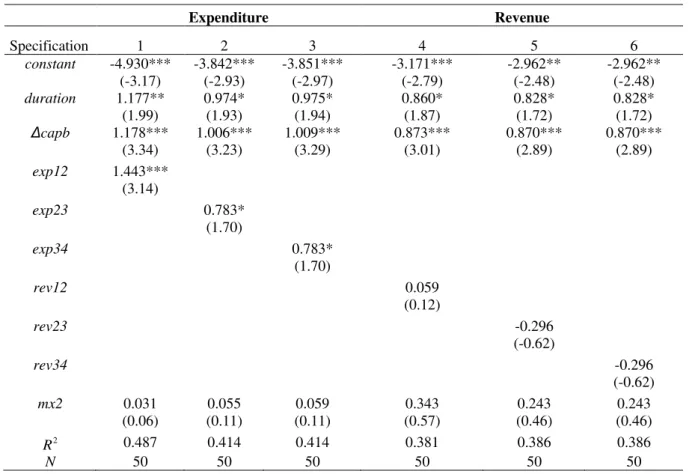
4.3. Measuring the success of fiscal consolidations

In this section we will investigate what the factors are that may contribute to the success

of fiscal consolidations. We computed dummy variables for successful fiscal adjustments in

two different ways based on the literature, in order to assess whether our findings are robust

across different criteria. The first measure (SUt1), is based on Afonso & Jalles (2012), who

define a fiscal consolidation as being successful, if the change in the cyclically adjusted

primary balance (∆bt) for two consecutive years is greater than the standard deviation (σ ) of

the full panel sample:

1 1

0 1,

0,

t i i t

if b SU

otherwise

σ + =

 _{∆ >}

 =  

∑

We have also included a measure computed by Alesina & Ardagna (2013) which is

based on the level of debt as a percentage of GDP. A fiscal consolidation is successful if the

debt-to-GDP ratio two years after the end of the fiscal adjustment (Debtt+₂) is lower than the

debt-to-GDP ratio in the last year of the adjustment (Debtt):

2 2 1,

0,

t t t

if Debt Debt SU

otherwise

+ < 

= 

 (5)

The identification of the leading policy option for the fiscal consolidation – either

expenditure or revenue based – is also assessed through dummy variables. Therefore, a fiscal

consolidation on period t is defined as being expenditure based (EXPt), if the change in the

total expenditure of the general government as a percentage of GDP in that period (∆expt)

accounts for a proportion greater than λof the change in the cyclically adjusted primary

balance (∆bt):

exp 1,

0,

t t t

if b EXP

otherwise

λ ∆

 _>

 _∆

= 

 . (6)

Following Afonso & Jalles (2012) we computed the composition of the adjustment for

three different thresholds, so that λassumes the values of 1/2, 2/3 and 3/4. A similar process

was conducted for the revenue based consolidations. Table VII shows the number of fiscal

consolidation episodes and their respective success rate (successes / total events), based on the

criteria defined in the earlier sections. The identification of the successful episodes follows

specifications (4) and (5). Table XX in the Appendix shows the successful fiscal episodes for

each country according to the different criteria.

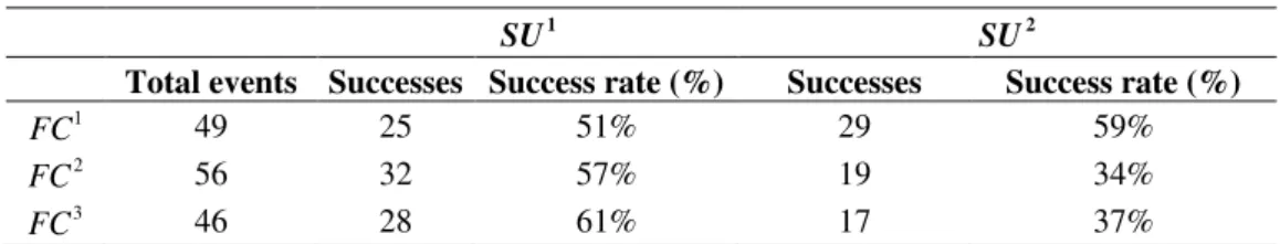
Table VII – Fiscal consolidation events and success rates

If we look at the successful events based on the change in CAPB for two consecutive

years, 1

SU , it can be seen that the success rates range from 51% to 61%, according to 1

FC

and 3

FC , respectively. Although 2

FC registers the highest number of successful

consolidations, the success rate is slightly lower than in 3

FC (57% vs 61%), and is thus

penalised by the higher number of consolidation events (56 vs 46). Nevertheless, success rates

are similar to the ones found in Afonso & Jalles (2012).

In the case of 2

SU , it can be seen that there are significant differences across the

criteria used to identify fiscal consolidations, namely between 1

FC and the remainder. This is

actually the only criterion that has a success rate which is similar to the one found in the 1

SU

case, whilst 2

FC and 3

FC are below their peers, by more than 20 percentage points.

On the one hand, the main explanation for the difference between the success rates

within 2

SU , has to do with the duration of the fiscal consolidations, coupled with its lower

flexibility, vis-à-visSU1. As seen earlier in Table I, the fiscal consolidations based on 1

FC

have a much higher duration than those of either 2

FC or 3

FC . The only requirement for a

fiscal consolidation to be successful according to 2

SU , is that the level of debt-to-GDP in two

years after the end of the adjustment has to be lower than the one in the last year of the

adjustment. Therefore, longer periods of adjustment will necessarily result in more successful

1

SU _SU2

Total events Successes Success rate (%) Successes Success rate (%)

1

FC 49 25 51% 29 59%

2

FC 56 32 57% 19 34%

3

FC 46 28 61% 17 37%

Source: author’s computations. Notes: SU1- Measure of success based on (4); 2

SU -

Measure of success based on (5).

years of fiscal consolidation. The same does not occur in 1

SU , as this allows for successful

and non-successful years within the same adjustment period.19

On the other hand, since the success rates based on 1

SU are generally higher than

those in 2

SU , one can argue that, based on these results, countries have been more successful

in improving their fiscal position rather than their levels of debt ratio. This points to the

possibility that, although there are improvements in the CAPB during fiscal consolidation

periods, this does not necessarily result in a fiscal surplus, at least during the two years

following on from the end of the adjustment. This ultimately impacts on countries’ debt ratios

during that period.

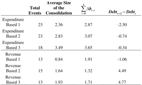
In Table VIII we present some facts about the expenditure and revenue-based

consolidations, which were computed for the three different criteria used to identify fiscal

contractions. By disentangling these, we can assess the possible differences regarding the

criteria used to define fiscal consolidations as being successful and also the possible

implications for GDP growth. This table shows the results computed for a threshold of λ

=2/3, while the results for the other thresholds can be consulted in tables XXI and XXII in the

Appendix.

Table VIII – Expenditure and revenue based consolidations: λ=2/3

Total Events

Average Size of the

Consolidation = + ∆

∑

0

t i i

b

2

t t

Debt₊ −Debt

Expenditure

Based 1 23 2.36 2.87 -2.50

Expenditure

Based 2 23 2.83 3.07 -0.74

Expenditure

Based 3 18 3.49 3.65 -0.34

Revenue

Based 1 13 0.84 1.91 -1.06

Revenue

Based 2 15 1.64 1.32 4.49

Revenue

Based 3 13 1.93 1.71 4.77

19 _{This is a consequence that derives from the fact that Alesina & Ardagna (2013) treat multi-year periods as a}

single episode and define all those years as either being successful, or not altogether, which might have some implications on the results. Perotti (2012) provides a detailed description of this issue.

Source: author’s computations.