© FECAP
DOI: 10.7819/rbgn.v16i50.1534
Subject Area: Finance and Economics
RBGN
The Impact of the 2008 Crisis on BM&FBovespa’s term Structure of
Conditional Correlations
O impacto da crise de 2008 na estrutura temporal de correlação condicional da
BM&FBovespa
El impacto de la crisis de 2008 en la estructura temporal de correlación condicional
de BM&FBOVESPA
Mauro Mastella1
Rodrigo Coster2 Received on January 17, 2013 / Approved on February 21, 2014
Responsible editor: André Taue Saito, Dr. Evaluation process: Double Blind Review
ABSTRACT
This article uses a BEKK-MGARCH model to identify the historical behavior of the term structure of covariance of the Brazilian BM&FBovespa stock exchange when compared to other exchanges in the American continent. The purpose of this research is to analyze the impact of the 2008 crisis on the cohesion of the Brazilian stock exchange when compared to the other exchanges in the sample. To this end, historical series were collected from five different stock market indexes ranging from the pre-crisis period until 2011. The bivariate modeling results indicate the presence of increased cohesion in the stock market indexes during the crisis period and the non-return of this cohesion to pre-crisis levels. They also indicate that, among the pairs analyzed, the pair of indexes IBOV x IPSA are the most appropriate choice for portfolio diversification.
Keywords: Multivariate GARCH. Conditional Correlation. Volatility.
1. Doctoral student at the Federal University of Rio Grande do Sul (UFRGS). Assistant professor at the State University of Rio Grande do Sul (UERGS). [mauro.mastella@ufrgs.br]
2. Master in Business Administration at the Federal University of Rio Grande do Sul (UFRGS). [rodrigo.coster@ufrgs.br] Authors’ address: Rua 7 de Setembro, 1156 – Centro – Porto Alegre – RS – CEP: 90.010-191 – Brazil
RESUMO
Este artigo utiliza uma modelagem BEKK--MGARCH para identificar o comportamento histórico da estrutura temporal de covariância da BM&FBovespa em relação às outras bolsas do continente americano. O objetivo da pesquisa é analisar o impacto da crise de 2008 sobre a co-esão da Bolsa brasileira relativamente às demais bolsas da amostra. Para isso, foram colhidas séries históricas de cinco diferentes índices bursáteis abrangendo desde o período pré-crise até 2011. Os resultados da modelagem bivariada indicam a ocorrência de um aumento da coesão entre os índices bursáteis durante o período de crise e o não retorno dessa coesão aos níveis pré-crise. Também indicam que par de índices IBOV x IPSA repre-senta a opção mais adequada para diversificação de portfólio entre os pares analisados.
RESUMEN
En este artículo se utiliza un modelado BEKK-MGARCH para identificar el comportamiento histórico de la estructura de covarianza temporal de la BM&FBOVESPA en relación a otros mercados del continente americano. El objetivo de la investigación es analizar el impacto de la crisis de 2008 sobre la cohesión del mercado de valores de Brasil en comparación con otras bolsas de muestra. Para ello, los datos históricos se han obtenido de cinco diferentes índices del mercado de valores que van desde el período precrisis hasta 2011. Los resultados del modelo bivariado indican la presencia de una mayor cohesión entre los índices bursátiles durante la crisis y el no retorno a la cohesión de estos niveles de precrisis. También indican que el par de índices IBOV x IPSA es la opción más adecuada para la diversificación de la cartera entre los pares analizados.
Palabras clave: GARCH multivariante. Correlación Condicional. Volatilidad.
1 INTRODUCTION
Volatility modeling in financial term series has gained a lot of attention since the emergence of seminal ARCH model in Engle’s article (1982). Since then, vast literature on the univariate models derived from ARCH has been published. Although the volatility of returns is at the center of this attention, understanding comovements in financial returns is also extremely important; in this way, Multivariate GARCH (MGARCH) models were reached.
One application for MGARCH models is the study of the relationships between different markets’ volatilities and covolatilities. In this way, answers to general questions about the behavior of markets are sought for. Does the volatility of a market cause volatility in other markets? Is the volatility of assets transmitted directly (through its conditional variance) or indirectly (through conditional covariances)? Does a shock in one market increase volatility in others? Are
correlations higher during high volatility periods? (LAURENT; BAUWENS; ROMBOUTS, 2006.)
This research aims at analyzing changes in correlations between markets over time, especially at the time of the 2008-2009 subprime crisis. Since volatilities between different assets move together in different markets, recognizing this characteristic by using multivariate modeling leads to more relevant empirical models than the use of univariate models separately. From a financial standpoint, this paves the way for better decision-making tools, such as asset pricing, portfolio selection, option pricing, hedging and risk management. For diversification of portfolios to be effective, it is necessary, for example, that the covariance between assets in the portfolio be fairly constant over time. Otherwise, changes in the term structure of covariances would lead to the need to readjust assets’ weights. Another desirable behavior is that correlations among assets or markets be low, for effective risk dilution.
This is no different in the Brazilian case. The volatility of Brazil’s stock market is interrelated to the volatility of other markets. In this sense, the objective of this research is to investigate changes brought about by the outbreak of the subprime crisis on the volatility relationships of BM&FBovespa with other exchanges in the Americas. To this end, historical series from five different stock market indexes ranging from the pre-crisis period to 2011 were collected. By means of a MGARCH model using a BEKK formulation proposed by Engle and Kroner (1995), the conditional covariances and correlation between the different stock markets were estimated and analyzed.
is also timely because it indirectly addresses the subject of decoupling, that is, the assumption that, in the post-crisis period, emerging economies’ financial markets would be separating themselves from major world markets, acquiring greater independence. The analysis of the term behavior of the Brazilian stock market’s correlations alongside the others may provide evidence regarding this hypothesis.
Recent publications seek to analyze the contagion effect. A multivariate GARCH approach is used by Frank and Hesse (2009) to analyze the spillover in emerging markets during the 2008 crisis, drawing on various financial variables such as banking spreads, sovereign risk and stock market indexes in developed and developing economies. The results brought evidence that contradicts the hypothesis of decoupling between markets. The work of Fenn et al. (2011) offers a comprehensive analysis of the correlation between 98 financial products between 1999 and 2010 using two different methodologies: the random matrix theory, to demonstrate that the correlation matrices are incompatible with random price changes; and principal component analysis, to demonstrate that a small number of components is responsible for a large proportion of variance within the analyzed markets. The authors demonstrate that there was an increase in the relationship between different markets following the 2008 crisis. Recently, Bouaziz, Selmi and Boujelbene (2012) analyzed the international transmission of the subprime crisis between the exchanges of the United States, France, Germany, Italy, the UK and Japan, using an MS-GARCH approach, finding evidence of volatility spillover only in the total analysis period and during the crisis.
However, it is beyond the scope of this research to study the contagion mechanism’s dominant factors. This work aims at analyzing the impact of the 2008 crisis on the term behavior of the correlation between American markets, focusing research on the Brazilian stock market’s correlations with other exchanges in the Americas, using a dynamic multivariate GARCH approach and timing of the crisis officially released by the
National Bureau of Economic Research. We intend, in this way, to find clues concerning the influence of the 2008 crisis on the relationships between the BM&FBovespa and the other stock markets that make up the sample.
In the following section we present the main concepts referring to MGARCH modeling. Next, we describe the research method and the data series used. Subsequently, the main results are discussed and the final considerations of this research are presented.
2 THE MULTIVARIATE GARCH MODEL
The MGARCH model is a natural evolution of the univariate GARCH models and is an option when you have two or more series and want to model not only their conditional variances, but also the cross effects (spillovers) of volatilities. However, one of its disadvantages are its many parameters, which increase exponentially as the number of series also increases. In an attempt to avoid this problem, several MGARCH models have been proposed, in which the main differences occur in the restrictions made to the model at time of estimation.
2.1 Definition
Introduced by Bollerslev and Wooldridge (1992), an M-varied GARCH (p,q) model (also known as vech Model) can be described as follows:
(1)
in which
corresponds to the conditional variance of series i over time. Since the models also allows for covariance estimation, will be defined as this covariance, that is,
(2)
where and are matrixes with d i m e n s i o n s
,
represents the operator stacking the lower triangular part of a symmetric matrix in a
vector and
is a vector
When we open the matrix operation for a GARCH(1,1) bivatiate case, we obtain
(3)
(4)
(5)
but the use of this model is unworkable
since the number of parameters is
, according to Bollerslev (2008).
2.2 Types of models
In an attempt to avoid the problem of the high number of parameters, various models based on MGARCH were proposed, and among them must be mentioned the diagonal vech and the CCC (constant conditional correlation). The restriction of the diagonal vech model – used in
the original MGARCH article – forces matrixes
Aiand Bj to become diagonal, so that, for the bivariate model with p = 1 = 1 model, the model obtained is:
(6)
(7)
(8)
The use of this restriction makes
become a function only of its lagged p-terms and of the crossed product of past q-lags of
. Thus, a criticism of this model is that past values of affect only its own conditional variance and its covariances, not interfering in the variance of the other series. Because of this restriction, the number of parameters of bivariate GARCH (1,1) is reduced from 21 to 9.
The CCC model, on the other hand, has no restriction as to the diagonalization of matrices, but states that the correlations should be constant over time, substituting equation (4)
for , with the remaining
equations showing no changes. This restriction reduces the num ber of required parameters for the covariance of a bivariate model to only 1 (p 12), reducing the total number of parameters in the model to 15.
2.3 Bekk
Presented by Engle and Kroner (1995), the BEKK model (Baba, Engle, Kraft and Kroner) introduces a way to calculate the covariance matrix (Ht). Instead of imposing restrictions on the VECH model, it suggests that the covariance matrix of an m-variate BEKK model (p,q) follow
where C is an inferior triangular matrix and and ,
are matrixes. For the BEKK-MGARCH (1,1) bivariate model we
The same as in the VECH model, the BEKK model has a large number of parameters . One solution to this problem is to restrict matrices B and A from being diagonal (LAURENT; BAUWENS; ROMBOUTS, 2006). Although its number of parameters is large, the model has a very attractive feature, which is non-restriction in its parameters. This freedom is due to the fact that the parameters enter the equation quadratically, thus avoiding negative variance estimates, as pointed out by Enders (2009). However, by forcing parameters to enter the equation quadratically, interpretability is lost, because the same parameter appears multiplying more than one factor.
3 DATA DESCRIPTION
For this research, we used the daily series of four Latin American market indexes: Índice Bovespa (IBOV) from Brazil, Índice de Precios y Cotizaciones (IPC) from Mexico, Índice Merval (Merval) from Argentina and Índice de Precio Selectivo de Acciones (IPSA) from Chile. We chose Standard & Poor’s 500 Index (S&P500) to represent the U.S. market.
Data was collected in the Yahoo Finance
site and series were formed based on closing values, with the necessary adjustments for dividends and splits, on each trading day. Initially index values from the 01/01/1998 to 12/31/2011 period were searched for. Daily rates were found for all indexes, except for the IPSA, whose quotes were only available after September 2003. Therefore, would obtain the following equations:
(10)
(11)
(12)
the period of analysis included only dates between 09/22/2003 and 12/29/2011. Moreover, the dates on which the values of certain indexes were not available were eliminated, leaving a total of 1,858 trading days in which the values were available for all indexes.
Next, the daily log returns for each index were calculated. These returns were then separated into three periods: the Pre-Crisis Period, between 01/10/2003 and 11/30/2007, with 943 returns for each index; the Crisis Period, between 12/01/2007 and 06/30/2009, with 354 returns for each index; and the Post-Crisis Period, between 07/01/2009 and 12/31/2011, with 560 returns for each index. These periods were chosen according to the Business Cycle dating Dating Committee of the National Bureau of Economic Research. This segregation is not obligatory to estimating the number of covariances, since the BEKK model is dynamic. An alternative to this separation into three periods could be intervention analysis – the name given to the methodology that suggests the use of proxy variables to indicate events that are external to the series. However, intervention analysis is useful only for modeling variations in the series’ average. Therefore, as the aim of this study is to examine whether there were also changes in the correlation structures of the series, we chose to model the three periods separately.
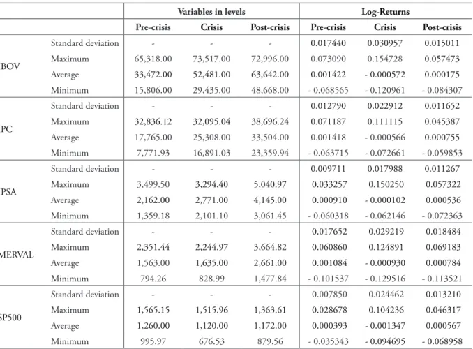
TABLE 1 – Descriptive statistics of the indexes in levels and their returns
Variables in levels Log-Returns
Pre-crisis Crisis Post-crisis Pre-crisis Crisis Post-crisis
IBOV
Standard deviation - - - 0.017440 0.030957 0.015011
Maximum 65,318.00 73,517.00 72,996.00 0.073090 0.154728 0.057473
Average 33,472.00 52,481.00 63,642.00 0.001422 - 0.000572 0.000175
Minimum 15,806.00 29,435.00 48,668.00 - 0.068565 - 0.120961 - 0.084307
IPC
Standard deviation - - - 0.012790 0.022912 0.011652
Maximum 32,836.12 32,095.04 38,696.24 0.071187 0.111115 0.045387
Average 17,765.00 25,308.00 33,504.00 0.001418 - 0.000566 0.000755
Minimum 7,771.93 16,891.03 23,359.94 - 0.063715 - 0.072661 - 0.059853
IPSA
Standard deviation - - - 0.009711 0.017988 0.011267
Maximum 3,499.50 3,294.40 5,040.97 0.033257 0.150250 0.057322
Average 2,162.00 2,771.00 4,145.00 0.000910 - 0.000102 0.000536
Minimum 1,359.18 2,101.10 3,061.45 - 0.060318 - 0.062146 - 0.072363
MERVAL
Standard deviation - - - 0.017652 0.029219 0.018484
Maximum 2,351.44 2,244.97 3,664.82 0.060860 0.124891 0.069183
Average 1,563.00 1,635.00 2,661.00 0.001084 - 0.000930 0.000784
Minimum 794.26 828.99 1,477.84 - 0.101537 - 0.129516 - 0.113521
SP500
Standard deviation - - - 0.007850 0.024462 0.013210
Maximum 1,565.15 1,515.96 1,363.61 0.028678 0.104236 0.046317
Average 1,260.00 1,120.00 1,172.00 0.000393 - 0.001347 0.000567
Minimum 995.97 676.53 879.56 - 0.035343 - 0.094695 - 0.068958
Source: the authors.
of models that are more complete than GARCH (1,1) did not provide more accurate predictions.
For data analysis, “R” version 2.13.2 software was used, complemented by the “mgarchBEKK” package, version 0.07-8. Through the use of package “mgarchBEKK”, parameters estimation is carried out by maximizing the quasi-maximum probability function and the Broyden-Fletcher-Goldfarb-Shanno (BFGS) numerical optimization method.
Next, we will discuss main research results.
4 RESULTS
Analysis of the term structure of the covariance between the rates of stock exchanges was carried out in pairs, always in conjunction with IBOV. This generated four GARCH (1,1) bivariate models (IBOV × SP500, IBOV × IPC, The data shows that the average returns
for the indexes in the crisis periods returns are lower than in the pre-and post-crisis periods. Considering the crisis period as a high volatility period, in certain indexes it is in this time interval that we find maximum and minimum values for returns. Moreover, the only index that had not yet reached again the maximum value of the pre-crisis period was the SP500.
IBOV × IPSA and IBOV × Merval), for each of the three periods, to allow comparison between the different estimates for the parameters and also between covariances. We chose to use the bivariate model facing a pentavariate model, due to the smaller number of parameters to be estimated (only 7 in each bivariate model, against 65 parameters in each pentavariate model). Each bivariate model was tested within each of the three periods, with cut-off dates obeying the official dating of the crisis according to the National Bureau of Economic Research.
The BEKK-MGARCH (1,1) equation used for modeling was described previously,
adapted from Laurent, Bauwens and Rombouts (2006), based on the seminal work of Engle and Kroner (1995). The Tables that present the results of parameter estimations were structured so that the IBOV is always represented by index 1 and the other exchange in the analyzed pair by index 2.
4.1 IBOV X SP500
The first pair of indexes assessed were IBOV and SP500. Table 2, below, presents the parameter estimates and the standard errors (in brackets).
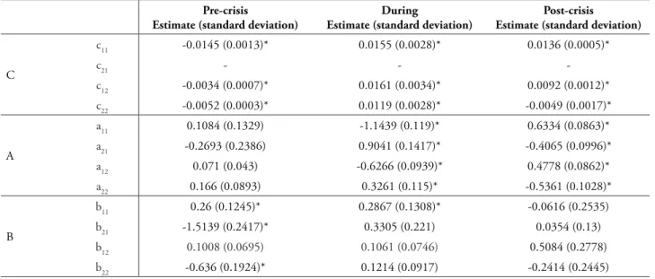
TABLE 2 – Bekk-Mgarch(1,1) results for IBOV X SP500
Pre-crisis
Estimate (standard deviation)
During
Estimate (standard deviation)
Post-crisis Estimate (standard deviation)
C
c11 -0.0145 (0.0013)* 0.0155 (0.0028)* 0.0136 (0.0005)*
c21 - -
-c12 -0.0034 (0.0007)* 0.0161 (0.0034)* 0.0092 (0.0012)*
c22 -0.0052 (0.0003)* 0.0119 (0.0028)* -0.0049 (0.0017)*
A
a11 0.1084 (0.1329) -1.1439 (0.119)* 0.6334 (0.0863)*
a21 -0.2693 (0.2386) 0.9041 (0.1417)* -0.4065 (0.0996)*
a12 0.071 (0.043) -0.6266 (0.0939)* 0.4778 (0.0862)*
a22 0.166 (0.0893) 0.3261 (0.115)* -0.5361 (0.1028)*
B
b11 0.26 (0.1245)* 0.2867 (0.1308)* -0.0616 (0.2535)
b21 -1.5139 (0.2417)* 0.3305 (0.221) 0.0354 (0.13)
b12 0.1008 (0.0695) 0.1061 (0.0746) 0.5084 (0.2778)
b22 -0.636 (0.1924)* 0.1214 (0.0917) -0.2414 (0.2445)
Source: the authors.
* Indicates a statistically significant coefficient at 5%. The coefficients presented here follow the form of the equation (9).
In general, the ARCH parameters (matrix A) were not significant in the pre-crisis period. That is, the volatility of the return of the indexes was little influenced by its last values. During this period, there is evidence that volatility had a minimum level (significant estimates in matrix C), and a persistence in variance and covariance structures (GARCH parameters, represented by matrix B).
During the crisis, the ARCH components became significant, indicating an immediate response to past returns of the index itself (IBOV or SP500) and also as to the past returns of
another index (SP500 or IBOV). The evidence that volatility maintained a minimum level remained. Analysis of the GARCH part points to the persistence of IBOV’s volatility only.
After the crisis, the indexes also showed a degree of influence established by their own returns and the returns of other index, as well as evidence of a constant level of volatility – however, no influence referring to their past variances and covariances.
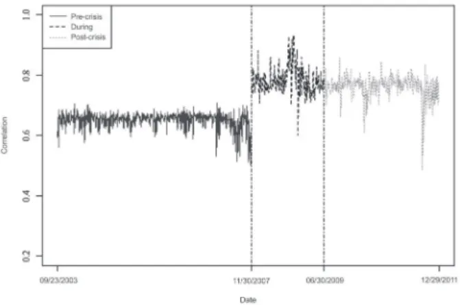
using the model shown in Equation 9, in each of the three periods. The correlation is an alternative to covariance representation, correcting it with the standard deviations of the two series and always varying between 1 and -1. To make visualization of the graph easier, the moving Average of the correlation values was represented with term window size equal to 1.
Analyzing Figure 1, we observe that the correlation between IBOV and SP500 indexes presented values closer to zero, with less variability, during the pre-crisis period. That is, if an investor wanted to hold portfolio diversification using the stocks that make up these indexes, he would find it harder in periods following the crisis. One can see that there was a change in the level of correlation over the crisis period, in which the average correlation increased from 0.649 to 0.783, indicating that markets varied in a more conjugated over the high volatility period. The average correlation remained virtually unchanged in the post-crisis period, when compared to the previous period, with an average of 0.759.
4.2 IBOV X IPC
The analysis of the second pair of indexes showed a slightly different ratio compared to the first pair analyzed. Table 3, below, presnets parameter estimates and their standard errors (in brackets).
FIGURE 1 – Behavior of the conditional correlation between IBOV X SP500 over time
TABLE 3 – Bekk-Mgarch(1,1) results for IBOV X IPC
Pre-crisis Estimate (standard deviation)
During
Estimate (standard deviation)
Post-crisis
Estimate (standard deviation)
C
c11 -0.0138 (0.0009)* 0.008 (0.0036)* 0.0072 (0.0023)*
c21 - -
-c12 -0.0012 (0.0012) 0.0174 (0.0017)* -0.0011 (0.0021)
c22 0.0024 (0.0025) 0.0009 (0.0072) -0.0003 (0.0011)
A
a11 -0.086 (0.0565) -0.9182 (0.1287)* 0.2277 (0.1156)*
a21 -0.4705 (0.0886)* 0.6568 (0.198)* 0.0771 (0.1525)
a12 0.1076 (0.0432)* -0.511 (0.1947)* 0.1765 (0.0917)
a22 -0.5449 (0.0563)* 0.3522 (0.2717) -0.3393 (0.1234)*
B
b11 0.3661 (0.0979)* 0.3671 (0.1548)* -1.21 (0.1419)*
b21 0.2187 (0.0791)* 0.5885 (0.2146)* 1.3348 (0.3596)*
b12 0.4619 (0.0912)* 0.1746 (0.0786)* -1.0973 (0.0433)*
b22 0.296 (0.1108)* 0.2778 (0.1425) 1.214 (0.1431)*
Source: the authors.
For this pair of indexes, the GARCH
component was significant during the
three periods analyzed, indicating a strong
persistence in volatility, both crossed (IBOV
×IPC) and not-crossed (IBOV x IBOV e IPC
× IPC). Over time, the ARCH components
were partly significant. We observed that
the cross-relationship between the returns
of the indexes was not relevant in the
post-crisis period, that is, markets failed to give
immediate responses referring to the returns
of the other exchange, responding only to
their own returns.
No specific relationship can be identified referring to the minimum levels of volatility, because the only parameter that remained significant over time was c11, indicating that only the volatility of IBOV had a non-zero level support.
It is noteworthy that we expected a decrease in the correlation between the series over the post-crisis period, a fact that is demonstrated in Figure 2. This reduction can be explained by the absence of evidence of cross-relationships between returns and volatility. Another relationship that is visible in Figure 2 is the increase in the correlation average over the crisis period (from 0.633 to 0.810) and the reduction of variability over this same period.
In this pair of indexes, the post-crisis period showed a decrease in average correlation (0.724), still higher than the pre-crisis levels and with greater variability than in the crisis period. That is, an investor who wanted to hold a portfolio diversification between these two markets would find it hard to do so, because of the high variability of correlations (pre- and post-crisis periods) or of the high value of the correlation (crisis period).
4.3 IBOV X IPSA
The analysis of the third combination of markets does not identify obvious cross-relationships between their volatilities, as shown in Table 4, in which are presented the parameter estimates and their respective standard errors (in brackets).
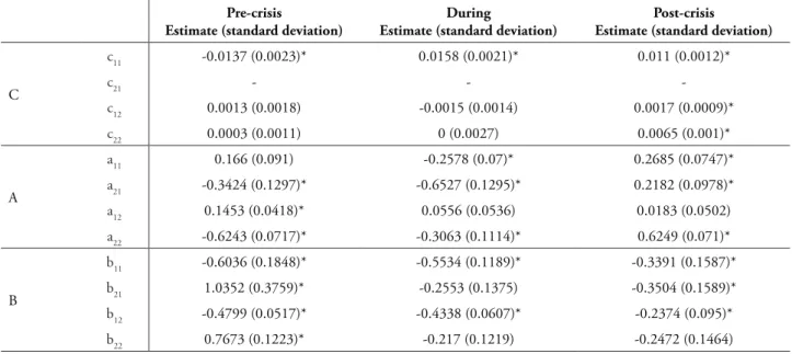
In the pre-crisis period, both the estimates of the ARCH and the GARCH parameters were, in general, statistically significant. However, in the three periods observed, no specific and lasting relationship can be identified referring to the minimum levels of volatility, because the only parameter that remained significant over time was c11, indicating that only IBOV’s volatility possessed a level with nonzero support, a behavior previously observed in other pairs of analyzed series.
Values found for the C matrix indicates that volatility had a constant nonzero level during the post-crisis period. Over that period, in general, the ARCH and GARCH parameters were also statistically significant, although it is not possible to identify a clear cross-relationship between the indexes.
TABLE 4 – Bekk-Mgarch(1,1) results for IBOV X IPSA
Pre-crisis
Estimate (standard deviation)
During
Estimate (standard deviation)
Post-crisis
Estimate (standard deviation)
C
c11 -0.0137 (0.0023)* 0.0158 (0.0021)* 0.011 (0.0012)*
c21 - -
-c12 0.0013 (0.0018) -0.0015 (0.0014) 0.0017 (0.0009)*
c22 0.0003 (0.0011) 0 (0.0027) 0.0065 (0.001)*
A
a11 0.166 (0.091) -0.2578 (0.07)* 0.2685 (0.0747)*
a21 -0.3424 (0.1297)* -0.6527 (0.1295)* 0.2182 (0.0978)*
a12 0.1453 (0.0418)* 0.0556 (0.0536) 0.0183 (0.0502)
a22 -0.6243 (0.0717)* -0.3063 (0.1114)* 0.6249 (0.071)*
B
b11 -0.6036 (0.1848)* -0.5534 (0.1189)* -0.3391 (0.1587)*
b21 1.0352 (0.3759)* -0.2553 (0.1375) -0.3504 (0.1589)*
b12 -0.4799 (0.0517)* -0.4338 (0.0607)* -0.2374 (0.095)*
b22 0.7673 (0.1223)* -0.217 (0.1219) -0.2472 (0.1464)
Source: the authors.
* Indicates a statistically significant coefficient at 5%. The coefficients presented here follow the form of the equation (9).
Figure 3, below, demonstrates another behavior that had already been observed in the pairs belonging to previous series: there is a clear change in the average correlation level during the crisis (from 0.477 to 0.666); in this case, however, the level shift comes with an increase in variability. Among the pairs of indexes analyzed, this was the one with the lowest average correlation over the three periods.
FIGURE 3 – Behavior of conditional correlation IBOV X IPSA over time
In this case, in the post-crisis period, the behavior not previously observed in the previous series was the reduction of the correlation’s resilience, that is, apparently, the correlation does not sustain a constant average over time. This represents an additional problem to investors who are interested in holding portfolio diversification across markets represented by these indexes, because it makes it even harder to maintain the assumption that the correlation matrices are fairly constant over time.
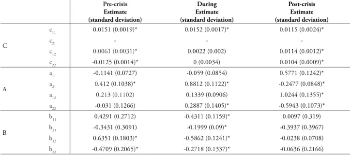
4.4 IBOV X MERVAL
TABLE 5 – Bekk-Mgarch(1,1) results for IBOV X MERVAL
Pre-crisis
Estimate (standard deviation)
During Estimate (standard deviation)
Post-crisis Estimate (standard deviation)
C
c11 0.0151 (0.0019)* 0.0152 (0.0017)* 0.0115 (0.0024)*
c21 - -
-c12 0.0061 (0.0031)* 0.0022 (0.002) 0.0114 (0.0012)*
c22 -0.0125 (0.0014)* 0 (0.0034) 0.0104 (0.0009)*
A
a11 -0.1141 (0.0727) -0.059 (0.0854) 0.5771 (0.1242)*
a21 0.412 (0.1038)* 0.8812 (0.1122)* -0.2477 (0.0848)*
a12 0.213 (0.1102) 0.1339 (0.0906) 1.0244 (0.1355)*
a22 -0.031 (0.1266) 0.2887 (0.1405)* -0.5943 (0.1073)*
B
b11 0.4291 (0.2712) -0.4311 (0.1159)* 0.0097 (0.319)
b21 -0.3431 (0.3091) -0.1999 (0.09)* -0.3937 (0.3967)
b12 0.6351 (0.1803)* -0.5862 (0.1241)* -0.0238 (0.0708)
b22 -0.4709 (0.2065)* -0.2718 (0.1337)* -0.0636 (0.2166)
Source: the authors.
* Indicates statistical significance for 5% coefficient value. Coefficients presented here follow the equation format (9).
identify two different sublevels of correlation in the crisis period (approximately 0.753 and 0.846), a characteristic that can only be observed because of the use of a dynamic model.
We would also like to add that, in the post-crisis period, there was a decrease in the average correlation to 0.718, still above the pre-crisis period. Compared to the previous pairs of indexes, this one showed high resilience during this period. In general, over the three periods analyzed,
the components of the model (level, ARCH part and GARCH part) were not significant for two consecutive periods. We observed that in the pre-crisis period the most obvious relationship between the indexes occurred at a level and that no obvious cross-relationship between the indexes can be identified.
In the crisis period, on the other hand, there was a clear persistence in volatilities, as proven by the significance of all matrix B parameters. However, no evidence that this relationship was maintained during the period immediately following were obtained. We noticed that in the post-crisis period we could again identify a relationship at minimum levels of volatility, as well as the emergence of a relationship in response to lagged returns, both crossed as well as not crossed. These changes in the characteristics of relationships between series hinder decision making by investors interested in portfolio diversification across these markets.
Figure 4 shows the term behavior of the correlation between IBOV and Merval. The pre-crisis period presented an average correlation of 0.531 and a gradually smaller variability over time. In the crisis period, the average correlation level rose to 0.798, a behavior already observed in previous series. In this case, however, we can
FIGURE 4 – Behavior of conditional correlation IBOV X MERVAL OVER TIME
4.5 Analysis of residuals
TABLE 6 – ljung-box test for standardized residuals (LAG = 20)
Model Exchange Pre-crisis During Post-crisis
test stat p-value test stat p-value test stat p-value
IBOV × SP500 IBOV 25.8655 0.1703 17.0546 0.6494 25.6993 0.176 SP500 24.3204 0.2287 66.1374 <0.001* 12.5802 0.8947
IBOV × IPC IBOV 20.7689 0.4108 11.0224 0.9456 17.3346 0.6311 IPC 33.6626 0.0285 31.7359 0.0462* 26.9989 0.1353
IBOV × IPSA IBOV 23.2867 0.2749 17.0546 0.6494 19.2287 0.507 IPSA 33.237 0.0318 26.8476 0.1396 39.2545 0.0062
IBOV × MERV IBOV 24.705 0.213 22.5484 0.3115 17.2228 0.6385 MERV 18.2339 0.572 26.2513 0.1577 37.8948 0.0091
Source: the authors.
* Indicates statistical significance for coefficient value at 5
5 FINAL CONSIDERATIONS
The analysis of a group of term series using multivariate models allows for the identification of cross-relationships between the series, which is not possible using various univariate models separately. Accordingly, the scope of this research was to evaluate the impact of the 2008 crisis on the term structure of BM&FBovespa’s conditional correlation when compared to other exchanges in the Americas.
This research yields results that do not support the hypothesis of decoupling, since the correlations continued to be high in the post-crisis period when compared to the pre-crisis period. The change in the term behavior of the correlation between BM&FBovespa compared to the other exchanges in the sample can be regarded as an indication of the occurrence of the contagion effect. The results found for the relationship between the U.S. exchanges are consistent with the results of other surveys conducted with data from other stock markets, such as Kim and Kim (2011), for the contagion effect between the U.S. market and Asian exchanges, and Fenn et al (2011) for the same effect in emerging markets, although the variables and the period of analysis are slightly different. The results of this study are also similar to Bouaziz, Selmi and Boujelbene (2012), who found a significant increase in the coefficients of dynamic correlation in the following pairs of The Ljung-Box test for standardized
residuals rejected the hypothesis of no autocorrelation in exchanges SP500 and CPI (highlighted with *), with a significance level of 5%, only in the period during the crisis. Other models with higher lags were tested for these exchanges; there was, however, no change the results of this test. This result does not invalidate the model, because, as demonstrated earlier, in these cases the parameter estimates were significant in most cases.
The results found in this analysis are consistent with the results of Lin and Chen (2010), in which the authors, to investigate the term behavior of the correlation between the markets of Tokyo and Hong Kong, also detected autocorrelation and found no significant differences in certain parameters in their model. However, since the structure of the model adopts a matrix form, we cannot rule out only a few estimated parameters.
exchanges: U.S.-France, U.S.-Germany, U.S.-Italy and U.S.-U.K.. In the Brazilian case, Perobelli, Vidal and Securato (2013) used an approach based on the stability of factor charges and also found signs of contagion for the subprime crisis.
In the present study, it is interesting to note that the 2008 crisis, even though it had its origins in the U.S. mortgage market, was able to change the term correlation structure of the Brazilian exchange as to the other exchanges in the Americas. Once the financial markets become increasingly integrated, the international mobility of capital allows investors to carry out the diversification of their investment portfolios in an international way, looking for assets that are little correlated so as to minimize risks. One consequence of this increasing internationalization of investments and interconnectivity of world trade is that, in times of turmoil for a certain economy, markets in other countries are also impacted. In the case of the 2008 crisis, this is no different, also generating impacts throughout the Americas.
In this sense, the use of BEKK-MGARCH (1,1) modeling, also used by Kim and Kim (2011), was adequate for achieving the proposed objectives. An important result found in every pair of series was the increased cohesion between stock market indexes during the crisis and the fact that this cohesion did not return to pre-crisis levels. That is, an investor who sought to diversify his portfolio would have advantages when doing so in the Brazilian and Chilean markets, because the pair of indexes IBOV × IPSA was the one that presented the lowest average correlation over the three periods.
On the other hand, the use of the same dates to establish the beginning and the end of the crisis period for all markets analyzed is a limitation in this study, since in some cases (e.g.: IBOV× IPC) the term behavior of the correlation seems to indicate that there was a change to the level of crisis in the days preceding the specified period, as observed in Figure 2.
Moreover, many of our analyzes and conclusions were possible only because of the use of dynamic multivariate modeling. In certain
cases, when studying correlations between markets, they are treated as constants. However, it has become a stylized finance fact that the correlations between the returns of assets or indexes are not constant over time, as previously documented by Erb, Harvey and Viscanta (1994), Longin and Solnik (1995) and Engle (2002).
Finally, the regulatory authorities of the Brazilian capital market should keep in mind the conditional correlations between international markets, so as to enhance the regulations and to structure effective ways of decreasing the risk of contagion by the Brazilian stock market. In this way, the quality of this capital market can be improved and further developed, aiming to attract non-speculative investments. In other words, the increase of international economic integration makes studies of contagion events relevant to the establishment of effective political-economic interventions by monetary authorities.
Taking the increased interconnection between American economies and Asian and European markets into account, future research can be carried out using a set of indexes that represents the overseas markets, in order to also examine the correlation of the Brazilian market with them. Moreover, a multivariate model that takes into account more than two levels simultaneously can be implemented to analyze the dynamic connections between a greater number of indexes, comparing the result with the modeling carried out here, although the number of parameters to be estimated will increase considerably.
REFERENCES
BOLLERSLEV, T. Glossary to ARCH (GARCH). Sept. 2008. CREATES Research Papers 2008-49.
______; WOOLDRIDGE, J. M. Quasi-maximum likelihood estimation and inference in dynamic models with time-varying covariances.
BORLAND, L. Statistical signatures in times of panic: markets as a self-organizing system. 2009. Available at: <http://arxiv.org/abs/0908.0111>. Acesso em: 03 jan. 2013.
BOUAZIZ, M. C.; SELMI, N.; BOUJELBENE, Y. Contagion effect of the subprime financial crisis: evidence of DCC multivariate GARCH models. European Journal of Economics, Finance & Administrative Sciences, [S.l], n. 44, p. 66, Jan. 2012.
ENDERS, W. Applied econometric time series.
Hoboken, NJ: John Wiley and Sons, 2009.
ENGLE, R. F. Autoregressive conditional heteroscedasticity with estimates of the variance of the United Kingdom inflation. Econometrica,
Oxford, v. 50, n. 4. p. 987-1007, July 1982.
______. Dynamic conditional correlation: a simple class of multivariate generalized autoregressive conditional heteroskedasticity models. Journal of Business and Economic Statistics, Alexandria,
v. 20, n. 3, p. 339-350, July 2002.
______; KRONER, K. F. Multivariate simultaneous generalized arch. Econometric Theory, Cambridge, v. 11, n. 1. p. 122-150,
Mar. 1995.
ERB, C. B.; HARVEY, C. R.; VISKANTA, T. E. Forecasting international equity correlations.
Financial Analysts Journal, Charllottesville, v.
50, n. 6, p. 32-45, Nov./Dec. 1994.
FENN, D. J. et al.Temporal evolution of financial market correlations. Physical Review E, New York, v. 84, n. 2, p. 1-15, Aug. 2011.
FRANK, N.; HESSE, H. Financial spillovers to emerging markets during the global financial crisis, Czech Journal of Economics and Finance, Prague, v. 59, n. 6, p. 507-521, Dec. 2009.
HANSEN, P. R.; LUNDE, A. A forecast comparison of volatility models: does anything
beat a GARCH(1,1)? Journal of Applied Econometrics, Chicester, v. 20, n. 7, p. 873– 889, Dec. 2005.
KIM, B. H.; KIM, H. Spillover effects of the US financial crisis on financial markets in emerging Asian countries. Apr. 2011. Auburn Economics Working Paper Series, with number auwp2011-04.
LAURENT, S.; BAUWENS, L.; ROMBOUTS, J. V. K. Multivariate GARCH models: a survey.
Journal of Applied Econometrics, Chicester, v. 21, n. 1, p. 79-89, Jan./Feb. 2006.
LIN, Y.; CHEN, Y. Study on time varying conditional correlations of stock market returns based on multivariate GARCH model. Advanced Management Science (ICAMS), 2010 IEEE
International Conference, July 2010. Available at: <http://ieeexplore.ieee.org/xpl/login.jsp?t p=&arnumber=5553092&url=http%3A%2F %2Fieeexplore.ieee.org%2Fxpls%2Fabs_all. jsp%3Farnumber%3D5553092>. Acesso em: 03 jan. 2013.
LONGIN, F.; SOLNIK, B. Is the correlation in international equity returns constant: 1960-1990.
Journal of International Money and Finance, Oxford, v. 14, n. 1, p. 3-26, 1995.
MOLDOVAN, I.; MEDREGA, C. Correlation of international stock markets before and during the subprime crisis. The Romanian Economic Journal, [S. l.], v. 14, n. 40, p. 173-193, June 2011.
PEROBELLI, F. F. C.; VIDAL, T. L.; SECURATO, J. R. Avaliando o efeito contágio entre economias durante crises financeiras. Estudos Econômicos, São Paulo, v. 43, n. 3, p. 557-594, jul./set. 2013.