BAR, Rio de Janeiro, v. 11, n. 1, art. 5, pp. 86-106, Jan./Mar. 2014
The Foreign Capital Flows and the Behavior of Stock Prices at
BM&FBovespa
Antonio Zoratto Sanvicente E-mail address: [email protected] Insper Instituto de Ensino e Pesquisa Rua Quatá, 300, 04546-042, São Paulo, SP, Brazil.
Received 9 November 2012; received in revised form 11 July 2013 (this paper has been with the authors for two revisions); accepted 22 July 2013; published online 2nd January 2014.
Abstract
The main purpose of this article is to investigate alternative explanations for the impact of foreign capital flows on Ibovespa returns, including: trend chasing, information contribution and mutual feedback. Daily data of the period between 2005 and 2012 are analyzed using simultaneous equation models which are estimated by ordinary least squares (OLS). Several exogenous market variables are included as determinants of returns and capital flows. The research results present that only the information contribution hypothesis is supported by the analysis. Besides, it also shows that the 2008 global financial crisis had no significant effect on the interaction of market returns with foreign capital flows.
Introduction
The knowledge of the relationship established between foreign capital flows and listed stock returns is unquestionably considered important for individual and institutional investors. Some articles recently published in the Brazilian financial press may be mentioned as a concrete evidence of the relevance and of the concern in that relationship. Anaya (2010), in his paper, conjectures prospects for stock price increases in the local market and also emphasizes the positions taken by a few market
professionals. Among them, the author quotes: “For Emy Shavo, a variable income security strategist
with J. P. Morgan, the prospects are for the return of a foreign capital inflow to the BM&FBovespa, a
determining factor in a more significant appreciation of assets in general” (Anaya, 2010, p. 16).
Subsequently, Valenti, Torres and Bellotto (2012), in a discussion of Brazilian stock market
prospects, state that “the foreign investor is still the main vector of trends at the local exchange”
(Valenti, Torres, & Bellotto, 2012, p. 12). Thus, a more detailed explanation is offered: “When he [the
foreign investor] enters the market, Ibovespa rises, ... and when he leaves, the market is left in
trouble”.
The same authors display a chart that would confirm the strong positive correlation between the
level of Ibovespa and the net cumulative flow (the cumulative difference between values of purchases
and sales) of foreign capital at BM&FBovespa.
The foreign capital flow reached its minimum worth in December 2008, i.e., –R$13,397 million,
after having reached R$11,991 million, in May 2008(1), a period in which Ibovespa dropped almost 50% of its points (from 72,592 to 37,550). The chart also shows that, starting in December 2008, the sign of the net cumulative flow became positive, while the level of Ibovespa rose to 69,304. And, to stress this point of view once more,
...when the large international investors buy or sell stocks in Brazil, the effects are shared by everyone [since they affect market prices], for better or worse [up or down]. And local asset
managers are left with the following understanding: ‘against the foreign capital flow there is no argument’ (Valenti et al., 2012, p. 16).
In the discussion of the interaction between foreign capital flows and local market returns, which occur in the local financial press, (as illustrated above), it is clear that the main concern is with the short-run interaction. It is also noticeable that there is a widespread belief that capital flows cause changes in market prices; and this belief is consistent with what is known in the theoretical literature, that is to say: foreign investors would tend to be more sophisticated and informed than other investors. However, as pointed out in the review of the theories, the relationship may also be recognized from price changes to capital flows, depending on the factor described as the trend chasing explanation.
Seen in these terms, the main objective of this paper is to concentrate on the nature, i.e., the direction, and on the significance of the short-run interaction, with the use of appropriate analytical tools, as well as with the investigation of daily data. The period analyzed in this research is fixed between Jan. 03, 2005 and July 31, 2012. Special attention is given to the possibility of a significant change in interaction as a result of the global financial crisis, which began in the second half of 2008. Candidate control variables are also used, since both, capital flows and market prices, which are proxied by Ibovespa, may be determined by and/or associated with various macroeconomic and market factors, and such as changes in exchange, interest rates, returns on international stock markets and stock market volatility, etc.
flows follow returns; therefore, foreign investment could be recognized as trend chaser. And, there is still the possibility that mutual feedback arises between returns with flows.
This paper is organized according to the following structure: second section discusses the relevant international and national theoretical literature. Third section explains the methodological approach to the analysis of the data, which, in turn, are described in fourth section, in terms of their definitions and sources. Fifth section presents and discusses the results; and, final section concludes and suggests possibilities for additional studies.
Review of Literature
The problem examined in this present paper is part of what is called the price-volume
relationship literature.
In his often cited paper, Hasbrouck (1991) suggests that the interaction of trades and quote revisions could be modeled as a vector autoregressive (VAR) system, because his tests using market
specialist-based data from the New York Stock Exchange (NYSE) indicated that a trade’s price impact
would arrive with a lag, the price impact being a positive but concave function of the trade size. However, he was discussing bid-ask spread revisions, and not the effect of trading volume on actual trade prices. Since he found that large trades tended to cause the widening of spreads, some authors attribute the idea of a positive relationship between contemporaneous trading volume and price changes to Hasbrouck (1991), such as, Sarwar (2005).
Using multiple linear regression analysis, Long (2007) presents evidences for the options market that duplicate existing statistics for a price-volume relationship in equity markets. Using 1983-1985 daily data for the Chicago Board Options Exchange (CBOE) market, he shows that a positive relationship exists between the absolute value of call price changes and the options trading volume; but that, as in the case of results for equity markets, demonstrates that positive call price changes are normally associated with significantly higher volume levels; otherwise, they are not connected to negative price changes. The discussions concentrate on the role of new information, as well as on the information arrival process. It is posited that the general result can be explained by a process of adjustment towards a new price equilibrium, after the arrival of new pieces of information that cause a change in the demand for security: when new, positive (negative) types of information cause an increase (decrease) in demand for a particular security, there is price increase (decrease) results; with this, the attendant volume of trading which was required tends to create a new equilibrium for prices.
McGowan and Muhammad (2011) examine the relationship between volume and price changes for spot and futures in Kuala Lumpur stock market index, using data since the inception of Malaysian futures market, in December 1995, until December 2003. They use cointegration analysis and find that trading volume and price changes present a significant long run relationship. They point out that most of the earlier empirical work focus on the contemporaneous relationship between trading volume and stock price changes, while more recent studies deal with the dynamic relationship, that is, the possible causality between price changes and trading volume.
Llorente, Michaely, Saar and Wang (2002) develop a model for the dynamic trading volume-return relation, with focus on individual stocks traded in US markets, instead of aggregates represented by stock market index. Their model emphasizes the influence of information asymmetry, which is proxied by bid-ask spread, company market capitalization and analyst coverage. They argue and test, with the expected results, that stocks which present low asymmetry (low bid-ask spreads, high market capitalization and extensive analyst coverage) will be the stocks that will be used in allocation or hedging decisions. In this case, large trading volume is not an informative signal, and, since volume does not lead to expected future stock payoff revisions, negatively autocorrelated returns will result. The opposite will happen with large trading volume signals for high informationally asymmetric stocks. In this case, large trading volume will be followed by positively autocorrelated returns, because the relevant body of information would be only partially incorporated into prices. This leads
Llorente et al. (2002) to test the impact of trading volume on the return autocorrelations.
Sarwar (2005) examines the role of the trading volume of S&P 500 options in the prediction of future volatility of the underlying index. Although that study covers the possible association between trading in one market (options) and prices in another (the underlying asset), it deals with the dynamic relationship between trading volume and price, that is, the eventual leads and lags in that relationship. It uses daily data from Jan. 04, 1996 to Aug. 31, 1997, for S&P 500 options traded on CBOE. The results indicate that options trading volume and index price volatility have a strong contemporaneous relationship. It also finds that previous options trading volumes have strong predictive ability for future price volatility. In addition, lagged volatility is also a significant predictor of future volume, and the author contends that these results are consistent with both hedging and information-related explanations for trading.
As for the hedging explanation, volatility would cause trading volume, because traders would revise their speculative or risk management activities upon observing changes in volatility. In the alternative (information) explanation, trading volume would cause volatility, because informed traders would prefer to use the options markets, due to their higher leverage and lower transactions costs. Hence, volume would become informative for volatility, and, after all, option pricing models require a volatility estimate.
Sarwar (2005) uses a two-equation simultaneous model, instead of the usual VAR approach commonly found in the empirical analysis, because VAR models do not account for the possibility of contemporaneous association. If that association is significant, then VAR models produce biased and inconsistent estimates for the structural dynamic relationships between trading volume and price changes, since there would be an important omitted variable problem.
However, although these above-quoted papers were important in the development of theory and methodology in the analysis of the price-volume relationship, none dealt with that relationship in an
international setting or in a situation in which the influence of a significant share of a market’s volume
had been considered.
An important reference on the relationship between foreign capital flows and local market
performance is Froot, O’Connell and Seasholes (2001). The authors examine the relationship between
Using the Froot et al. (2001) approach, Gonçalves and Eid (2011) performed a similar analysis (covariance decomposition and VAR model estimation), with more recent data, focusing exclusively
on the Brazilian market. As Froot et al. (2001, p. 155) had pointed out before, “the closest [main area
of work on which their paper was built] is probably the small literature focused on international
portfolio flows”, but those studies had at most used monthly or quarterly data.
Gonçalves and Eid (2011), in turn, based their hypothesis and analytical approach on Froot et
al. (2001), and the literature they mostly referred to is a financial contagion literature, which is represented by Marçal, Pereira, Martin and Nakamura (2006) work.
Their study used daily BM&FBovespa data from December 2001 to December 2009. In order to account for the onset of the 2008 global financial crisis, the authors estimated three different types of VAR models: (a) before the crisis; (b) during the crisis period (after Sep. 11, 2008); and (c) the full crisis period. In other words, no formal test for the impact of the crisis on the price-capital flow relationship was implemented, such as the use of dummy variables.
The results indicate that there is evidence for information contribution as well as for feedback trading (their term for flows following returns, i.e., for trend chasing). In particular, it must also be pointed out that their analysis examined the interaction between price changes, purchases and sales separately, and not the difference between purchases and sales, which clearly seems to be the variable of concern to market professionals and the press.
Before presenting the methodology employed in this paper in next section, the paper’s contributions must be highlighted: (a) it uses the difference between purchases and sales as the proxy
for capital flows, instead of analyzing purchases and sales separately(2);(b) the VAR model approach
is replaced by a more appropriate technique, in order to avoid the use of a possibly biased and inconsistent estimator of the price-capital flow relationship, since contemporaneous correlations are
significant(3); (c) the period of coverage is extended to mid-2012, making it possible to include a long
and representative period following the onset of the global financial crisis; (d) the eventual effect of the crisis on the price-capital flow relationship is explicitly taken into account through the use of an appropriate dummy variable structure, in contrast to the variable structure which is used in Gonçalves and Eid (2011). Meurer (2006), however, may be the pioneering study attempting to examine the interaction of foreign capital flows (measured as the difference between stock purchases and sales, or FLV) and stock market prices in Brazil, represented by Ibovespa. Monthly data from January 1995 to July 2005 were used. In the analysis, the performance of the S&P500 index, the 3-month U.S. T-bill rate, the local market interest rate, proxied by SELIC rate, the Real/US dollar exchange rate and the country risk spread for Brazil, represented by EMBI+ spread, are used as additional candidates for explaining the interaction between capital flows and stock market prices. In addition, a measure of stock market liquidity is used, represented by the average monthly volume traded at Bovespa. It is claimed that there could be a positive relationship between market liquidity and index level, but no reference to the literature is offered in support of such a claim(4). Also, since it seems clear that trades by foreign investors are reflected in the overall trading volume, it is possible to, at least, wonder how much incremental power would be in overall market liquidity, when a large part of it is accounted for by foreign capital flows themselves. The results indicate that stock market prices are clearly affected by exchange rate, country risk spread and market liquidity. Related to capital flows and to their interaction with Ibovespa, this paper concludes that flows seem to affect the index and to be affected by the index, and it also proposes an explanation based on investment strategies by foreign investors. At any rate, the conclusion is that the effect of flows on the index appears to take place through liquidity. Since flows and liquidity tend to be highly correlated, it is not clear whether returns are influenced mostly by foreign capital flows or by domestic liquidity. The paper also suggests that further studies consider using data with different frequencies, and, since this present paper uses daily data in an analysis of the same phenomenon, it is one of its own contributions to the literature.
decrease after prices rise, and, therefore, they cannot cause the index. In this paper, instead of a direct measure of capital flows, as the FLV measure in Meurer (2006), the authors use the CVM-provided bstatistics of foreign investor share in total market capitalization. This was also used in Meurer (2006) as his PART measure.
Ferreira and Zachis (2012) examine the significance of the association between jumps in the returns on Ibovespa portfolio and jumps in the local market interest rate, the exchange rate and the country risk spread, measured by C-Bond spread. An international market index is also used, in the form of Dow Jones Industrial Average (DJIA). Daily data collected from January 2, 2001 to October 25, 2005 are used as well. Although this is one of the few papers in Brazilian literature which has used daily data, it does not contemplate any explanation about foreign capital flows into or out of the market; or any account of their effect on the stock market index. It concludes that co-jumps with the C-Bond spread are more important than with those in the DJIA.
One of the possibly relevant issues, in particular for the methodology used in this paper, and some appropriate data definition criteria, particularly for the dating of the global financial crisis and the choice of values for the crisis dummy variable used later on, are identified exactly when the crisis began. The literature, however, is not clear on this matter, as indicated by the attempts to verify whether the results of any specific study are strong to such a choice. The results reported below indicate that either (a) a robustness exercise is required, or (b) any reasonable choice in the 2007-2008 period would be sufficient.
Chor and Manova (2010) date the global financial crisis from September 2008 (into the cliff) to August 2009 (back from the cliff) in a study that concerns with how sensitive the volume of international trade seemed to be in a relation with the changes in external credit conditions caused by the crisis. The dependent variable is measured with the monthly series of the cost of external finance. The paper explicitly considers other candidate data for the beginning and the end of the crisis. For example:
While nervousness over the exposure of financial institutions to the subprime mortgage market had been building up steadily since the end of 2007, two events in September 2008 – the
collapse of Lehman Brothers and the government bailout of AIG – brought credit activity to a
virtual standstill (Chor & Manova, 2010, p. 5).
Later on, they indicate that their results were robust to the choice, for example, of March 2008 as the starting point for the crisis (the Bear Stearns collapse). This seems to justify the use of any data in the present paper, provided it is already in the 2007-2008 range.
Alper, Forni, and Gerard (2012) analyze the behavior of sovereign credit risk prices, with credit default swap (CDS) and relative asset swap (RAS) spreads. The goal was to identify the market in which credit risk price discovery took place. And the results indicate that this occurs in CDS market. They use monthly data from January 2008 to January 2011 which are collected in 21 developed economies with the random-effect panel methodology. As in Chor and Manova (2010), various events are used as crisis dating markers: the Bears Stearns collapse in March 2008, the Lehman Brothers debacle in September 2008, the Greek crisis, starting in November, 2009, and the IMF-EU assistance program following the Greek crisis of May 2010. In the analysis, however, all the crisis and assistance program dummy variables are used together, instead of alternatives for dating a single crisis. Another
important categorical variable – the announcement of FED bond purchases in March 2009 – was
Methodology
Regarding the interaction of capital flows with market prices, two approaches were commonly used: (a) non-conditional interaction analysis, through covariance decomposition; (b) conditional
interaction analysis, with the use of VAR models. Both approaches were used in Froot et al. (2001)
and in Gonçalves and Eid (2011).
As the name indicates, covariance decomposition refers to the interaction of flows and returns
without controlling other determining variables, i.e., variables which could explain either flows and/or
trading volume, on one hand, and changes in stock market prices, such as changes in interest rates, exchange rates and other asset market prices, on the other. In this sense, it is only a descriptive and not inferential tool, and it is not employed in this paper.
Alternatively, VAR models are used to represent and to test the strength of dynamic interactions between the two variables of interest (flows and returns), with the determination of an appropriate number of leads and lags with the use of Granger causality tests (Granger, 1969). However, as pointed out by Sarwar (2005), the possibility of significant contemporaneous correlation between flows and returns would lead to the omission of a variable which represents contemporaneous values for those (endogenous) variables and, for this reason, they would be excluded from a VAR model, estimating a VAR model that would be equivalent to the use of a biased and inconsistent estimator. A more appropriate alternative, as suggested by Sarwar (2005), is to estimate simultaneous equation models, such as:
1 0 0
t
k m n
t Fj t j Fj t j F i F it Ft
j j i
F
F
R
X
t = 0,1,…,T(1)
(2)
1 0 0
t
k m n
t Rj t j Rj t j Ri Rit Rt
j j i
R R F X
t = 0,1,…,T
In equations (1) and (2):
. Ft = a measure of capital flows (for example, the difference between foreign purchases and sales)
on day t;
. Rt = rate of return on the market portfolio on day t;
. Xit = a vector of n determining variables for either Ft and Rt, as listed in the next section.
For estimation purposes, the appropriate number of lags (k and m, not necessarily equal in both equations) for each equation is determined on the basis of autocorrelation and cross-correlation tests of residuals from alternative specifications of equations (1) and (2), i.e., alternative numbers of lagged terms for the endogenous variables. The components of XFit and XRit are proposed on the basis of
results already available in the literature for explaining either Ft (such as Gonçalves & Eid, 2011) or Rt
(see, for example, Sanvicente, 2004). The terms αF0 and αR0 in equations (1) and (2), respectively,
represent the inclusion of the possible contemporaneous relationship between flows and returns, in equation (1), and returns and flows, in equation (2). The same can be said of corresponding terms for
the contemporaneous relationships with other variables, used as control variables(5).
The main hypotheses tested in this paper correspond to the following results when estimating (1)-(2):
Trend chasing hypothesis: flows follow returns. This result will be substantiated if {αFj, j > 1}
are positive and significant.
Information contribution hypothesis: returns follow flows. This result will be substantiated if
{αRj, j > 1} are positive and significant.
Of course, according to previous results in the literature, the two explanations may be
simultaneously valid, and this conclusion will be supported if both {αFj, j > 1} and {αRj, j > 1} are
positive and significant.
Data Definitions and Sources
Foreign capital flows and market returns
The main variables used in the data analysis are the net flow of foreign investment at BM&FBovespa; and the rates of return on the round lot segment of the stock market at that same exchange, which was the only one in operation in Brazil during the period studied. Therefore, the capital flows that are considered in this paper cover 100% of this type of activity by foreign investors
from all the countries in Brazilian market, as opposed to what was possible, for example, in Froot et
al. (2001), who relied on data provided by a single, albeit important U.S. custodian, for a substantial
share, but not the totality of U.S. investors, and mainly U.S. investors.
The daily series of purchases, sales and, thus, the net flow of foreign investment at BM&FBovespa, for the period from January 03, 2005 to July 31, 2012, were kindly provided by the
exchange’s Communications Department. In turn, the daily series of Ibovespa level were downloaded
from Economática database. The actual series used was the average value of the index on each day, or IBOVMED.
The components (purchases and sales) of daily capital flows (NETFLOW) were first adjusted by the level of Ibovespa on each corresponding day, in order to exclude the effect of price changes on flow values, as recommended by Gonçalves and Eid (2011). In addition, the measure of trading activity, proposed by Lakonishok, Shleifer and Vishny (1992) and adopted by Gonçalves and Eid (2011), was also used here. Specifically:
t t t
t t
P S
F
P S
Where,
. Pt = purchases on day t and St = sales on day t, after the adjustment by the average level of
Ibovespa on the same day(6).
. Finally, the foreign capital flow data used in this paper correspond to trades executed on each day
Control variables
Most of the control variables are proposed in the already reviewed literature, and they include:
EMBI = Brazilian risk spread, calculated in J. P. Morgan’s Emerging Markets Database Index
(EMBI), as a proxy for an important systematic risk factor in the Brazilian market. Sanvicente (2004) reports a significantly negative correlation between changes in the spread and the prices of Brazilian stocks traded in the local market. This variable was obtained from Datastream/Thompson Reuters database. As constructed in EMBI methodology, this series is the daily value of a total return index. This means that the relationship between the risk spread and the value of the index is negative: when
the country debt risk increases, the value of that country’s debt securities decreases, and, hence, the
value of the index also falls.
Therefore, to a negative relationship between spread and Ibovespa there corresponds a positive relationship between the value of the EMBI index and the Ibovespa.
S&P500 = level of Standard & Poor’s 500 index of U.S. market stocks, as a proxy for the value of a portfolio in the most important alternative market for investment allocation by foreign investors. Again, Sanvicente (2004) reports significant positive correlations between changes in S&P 500 and the prices of Brazilian stocks traded in the local market. The direction of the relationship between changes in S&P500 and net flows into Brazilian stock market is indeterminate; it may be the case in which a better performance of U.S. stock market would drive investors to that market and away from Brazilian market; however, a better performance of U.S. equity market would also be a signal of better performance in equity markets in general. The evidence that there is positive contemporaneous correlation between S&P500 and Ibovespa returns points to the second explanation. The source of values for S&P500 is Economática database.
TBILL3m = level of 3-month U.S. Treasury bill rate, as the basis for the opportunity cost for foreign investors. The source of this variable is Datastream/Thompson Reuters database. This variable is the so-called secondary middle rate, that is to say, the average rate observed in the secondary market for Treasury bills on any day. In Datastream database, FRTBS3M series is used. The lower the rate, the stronger the incentive to invest in riskier markets, such as the stock markets of emerging nations. Therefore, a negative relation would be expected between changes in TBILL3m and the flow of foreign capital into BM&FBOVESPA.
CDI = overnight interest rate in Brazil, on a daily basis, as a proxy for the risk free rate in the local market, and as a candidate for a component of the required return on all risky assets for local investors. The data were downloaded from Economática database, and the variable is measured as the daily change in Economática CDI OVER index. A negative correlation between changes in CDI rate and Ibovespa returns may be expected, both from the pricing model argument and from the expectation that investors would reallocate their investments from equities to fixed income instruments if the rates of interest that these investors could command had increased.
PTAX = exchange rate between Reais and US dollars, a proxy for the rate at which foreign investment money could be converted into and out of the local currency. The series for this variable was obtained in Economática database. A negative relationship with market returns is expected,
according to results presented in Sanvicente’s work (2004).
VOLAT = Daily estimated volatility of the local stock market. This volatility was measured, as in Gonçalves and Eid (2011), by computing the difference between daily maximum and minimum values of Ibovespa, and then dividing the resulting difference by the average value of index on the same day. Since this is a proxy for market risk, negative relationships are expected both for capital flows and for returns.
included to represent the fact that trading in ADRs competes with trading in the local market and it could cause a reduction in local trading(7). The inclusion of this variable results from a conjecture proposed by Froot et al. (2001).
Lastly, a dummy variable is included, in order to permit the evaluation of whether and how the 2008 global financial crisis affected the price-capital flow relationship. The dummy variable takes on the value of zero, from January 03, 2005 to September 15, 2008, and it also takes on the value of one,
from September 16, 2008 on(8). In addition to an intercept dummy, dummy variables for slope
coefficients are created for lagged values of Rt and Ft.
Descriptive statistics
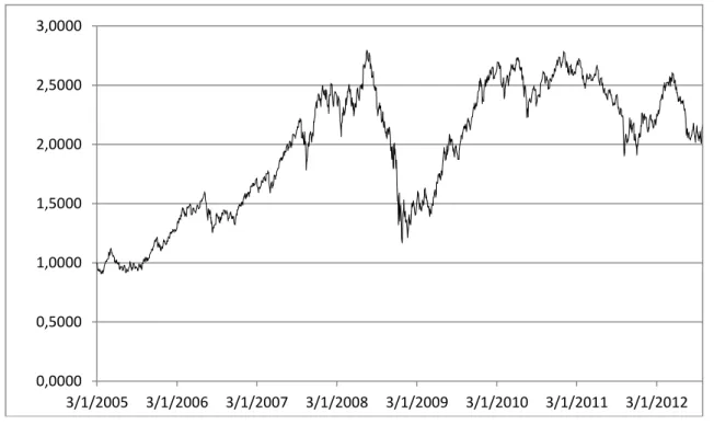
The actual daily series of Ibovespa level and capital flows (purchases minus sales, adjusted for Ibovespa level) are displayed in Figures 1 and 2, respectively. Ibovespa series was converted into an index equal to 1,000 as of January 03, 2005.
Figure 1. Ibovespa Level, 2005-2012 (Jan. 03, 2005 = 1,0000). Source: Developed by the author.
Figure 1 shows that the nominal value of Ibovespa rose approximately 100% in the seven and a half years of the period under study, and it also clearly indicates a larger than 50% drop from mid-May 2008 to the end of the same year. However, as previously mentioned, this paper, for practical purposes, presents the beginning of the global financial crisis in September 15, 2008 (Lehman Brothers collapse). Until the end of July, 2012 (a little over four years later), the nominal value of the index had not been completely recovered.
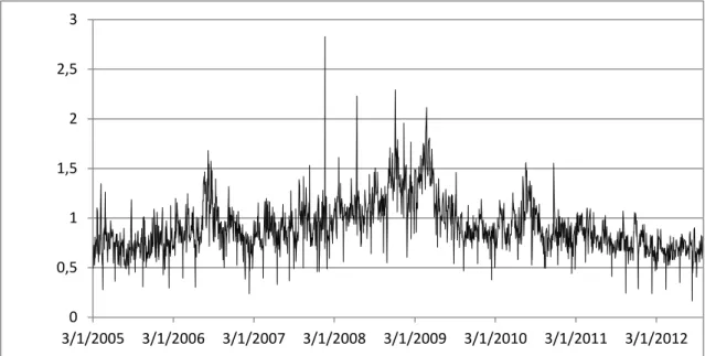
Figure 2 indicates that, until approximately mid-2007, capital flows had a constant, but a smaller volatility than that observed during the height of the financial crisis. Five extremely negative
flows are observed in this full period (defined as days on which Ft was lower than -0,30), and three of
these most extreme negative flows occurred before the onset of the 2008 crisis.
0,0000 0,5000 1,0000 1,5000 2,0000 2,5000 3,0000
Figure 2. Capital Flows Adjusted for the Level of Ibovespa, 2005-2012. Source: Developed by the author.
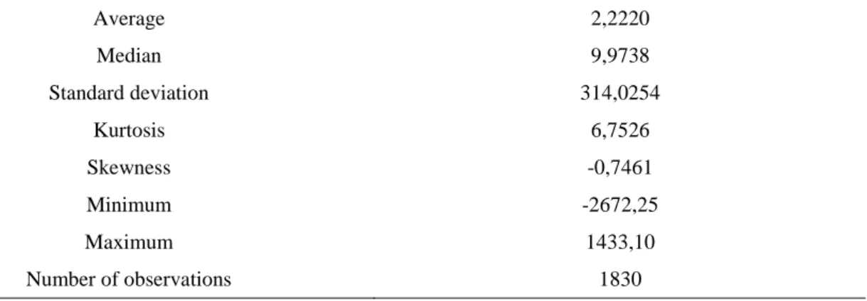
Table 1 provides descriptive statistics for the actual series of differences between purchases and sales by foreign investors (not adjusted by Ibovespa).
Table 1
Descriptive Statistics: Capital Flow (in Millions of Reais), Unadjusted for the Level of Ibovespa), 2005-2012
Average 2,2220
Median 9,9738
Standard deviation 314,0254
Kurtosis 6,7526
Skewness -0,7461
Minimum -2672,25
Maximum 1433,10
Number of observations 1830
Note. Source: Developed by the author.
Table 1 shows that the average daily flow is barely greater than zero, and it also presents some negative asymmetry. The largest negative flow, of more than 2,5 billion Reais occurred on December 02, 2008, that is to say, it occurred when the brunt of the crisis was unfolding(9).
Table 2, in turn, displays descriptive statistics for the proportion of total foreign capital flows
(purchases + sales) relative to the total volume of trading in the round lot segment of the exchange’s
stock market(10).
-0,8 -0,6 -0,4 -0,2 0 0,2 0,4
Table 2
Descriptive Statistics: Proportion of Total Foreign Capital Flows (Purchases + Sales, Unadjusted for Ibovespa Level) as a Proportion of the Total Volume of Trading, 2005-2012
Average 0,7913
Median 0,7785
Standard deviation 0,1374
Kurtosis 56,7496
Skewness 4,6427
Minimum 0,4786
Maximum 3,0585
Number of observations 1830
Note. Source: Developed by the author.
Figure 3, presented below, clearly shows that the trading of ADRs is an important phenomenon, justifying the inclusion of a control variable in the model. In fact, the average proportion, during the period, was slightly higher than 90%, often higher than 100% of local market volume, and never lower than 16,5%.
Figure 3. Trading in ADRs of Brazilian Firms as a Proportion of the Volume of Trading at the
Exchange, 2005-2012.
Source: Developed by the author.
Finally, as justification for the way the problem was adjusted to the estimation purposes, it must be considered that the coefficient of correlation between daily returns and daily capital flows (adjusted for Ibovespa level) was equal to 0,2933, during the period under analysis.
0 0,5 1 1,5 2 2,5 3
Results
Before estimating the model initially described by the system of equations (1)-(2), Augmented Dickey-Fuller (ADF) unit root tests were performed in order to evaluate whether one is dealing with stationary series, including daily Ibovespa returns and capital flows, and also all the candidate control variables described above. The appropriate transformations – i.e., first differencing or application of log returns – were implemented as necessary. The testing of the trend chasing versus information contribution hypothesis was implemented with the following operational version of equations (1) and (2):
7 7
,
1 0 1
7 7
n
t Fj t j Fj t j F i Fit Ft
j j i
F
F
R
X
(3) 7 7 ,1 0 1
n
t Rj t j Rj t j R i Rit Rt
j j i
R R F X
(4)In equation (3), i = RS&P500 and RPTAX; in equation (4), i = RS&P500, DEMBI, RPTAX, DTBILL.
Augmented Dickey-Fuller (ADF) test results, reported in Table 3, indicate that, since all variables had unit roots, they were converted into stationary series, either by first differencing or by the calculation of log returns. The former solution was used for the original variables defined as EMBI, TBILL3m, VOLAT, and CDI. Log returns were used for the S&P500, PTAX and ADRSHARE variables. Market returns, calculated as the log returns using the daily average value of Ibovespa, were found not to have unit roots, and the RIBOVMED variable was thus defined and used for representing R; capital flows, represented by the NETFLOW variable, were found to have unit roots as well, and were first differenced, creating a DNETFLOW dependent variable, standing for F in equations (3)-(4).
Table 3
Stationarity (ADF) Test Results – from January 03, 2005 to July 31, 2012 (1830 Observations)
Variable Lag length t-ADF Prob. ADF
RIBOVMED 1 -31,1287 0,0000
DNETFLOW 12 -19,2570 0,0000
RPTAX 0 -42,6368 0,0000
DEMBI 0 -34,9785 0,0000
DVOLAT 7 -23,8875 0,0000
DTBILL 2 -30,0451 0,0000
RADSHARE 8 -22,3904 0,0000
DCDI 0 -43,0268 0,0000
RSP500 0 -48,7172 0,0001
Note. The tests included a constant term and one lag, in all cases, with a maximum number of 24 lags. Number of lags based
As indicated in Table 3, all variables are integrated of order 1, I (1), and it is important to check the possibility that some linear combination of two or more variables would produce a large error. In other words, if the variables are linked, for example, through a pricing relationship, if their linear combination does not correspond to a market equilibrium or does not respect arbitrage restrictions, it would be necessary, for such an error, to be quickly corrected. This verification is done through a cointegration test. Table 4 provides the results of such a test, and it indicates that, with the maximum eigenvalue test, at 1%, there are two cointegrating relationships.
Table 4
Cointegration test – from January 03, 2005 to July 31, 2012 (1830 Observations). Variables: LNIBOV, LNPTAX, LNSP500, LNADRSHARE, TBILL, CDI, EMBI
Number of cointegrating vectors
Eigenvalue Maximum eigenvalue statistic
Probability
None 0,095668 183,5917 0,0000
At most one 0,066639 125,8582 0,0000
At most two 0,024685 41,6155 0,0108
At most three 0,018958 34,9304 0,0373
At most four 0,009165 16,8027 0,5969
As mentioned before, two error correction equations were estimated and used for the
computating the corresponding error correction terms, EC1 and EC2:
EC1 = -5,5316 + LNIBOV – 0,0013 EMBI + 6,5519 VOLAT + 0,0765 TBILL + 1,7509
LNADRSHARE – 0,0045 CDI – 1,6066 LNSP500
EC2 = -65,5896 + LNPTAX + 0,0036 EMBI + 41,7068 VOLAT + 0,0103 TBILL + 2,7694
LNADRSHARE + 0,0963 CDI + 2,6638 LNSP500
A further consideration in this paper is the possibility of a change in the nature of the interaction between market returns and changes in capital flows, which was possibly caused by the 2008 global financial crisis. Hence, a dummy variable analysis was performed, as follows: a categorical variable,
CRISISt was created with the following structure. Its value is set equal to zero if the data fall in the
Jan. 03, 2005 to September 12, 2008 period, and 1 otherwise. Because the interest was on possible changes in the interaction between the two endogenous variables, slope dummy variables are, then, defined as CRISISt x DNETFLOWt or CRISISt x RIBOVMEDt. This was applied to the first five
lagged values of both endogenous variables.
Table 5
Estimation of Equation (3) by OLS, with Data Collected from January 03, 2005 to July 31, 2012. Dependent Variable: DNETFLOW (1824 Observations)
Variable DNETFLOW equation t statistic
Intercept -0,0010 -0,2207
DNETFLOW(-1) -0,6370* -27,0763
DNETFLOW(-2) -0,4732* -17,3213
DNETFLOW(-3) -0,3125* -11,1434
DNETFLOW(-4) -0,1913* -7,1156
DNETFLOW(-5) -0,0404 -1,6381
CRISIS 0,0004 0,0355
CRISIS*RIBOVMED -0,3061 -1,3118
CRISIS*RIBOVMED(-1) 0,0612 0,3721
CRISIS*RIBOVMED(-2) -0,4636 -1,9599
CRISIS*RIBOVMED(-3) -0,1759 -0,9084
CRISIS*RIBOVMED(-4) -0,0122 -0,0863
CRISIS*RIBOVMED(-5) -0,2920 -1,3571
RPTAX 0,6495* 3,0560
RPTAX(-1) 0,1889 0,9331
RPTAX(-2) 0,5577 2,6206
RSP500 0,8787* 5,7150
RSP500(-1) 0,4875 2,3952
RSP500(-2) 0,2080 0,9599
RIBOVMED 1,8445* 9,2184
RIBOVMED(-1) -0,0157 -0,2611
RIBOVMED(-2) 0,3686 1,6730
RIBOVMED(-3) -0,1604 -1,0908
RIBOVMED(-4) -0,3456 -2,0679
RIBOVMED(-5) -0,1417 -1,0422
EC1 -0,0002 -0,0604
EC2 0,0049 1,9512
Adjusted R2 0,3925
Durbin-Watson statistic 2,0112
F statistic 45,2271
Prob(F) 0,0000
Note. Source: Developed by the author.
* Significant at the 1% level.
increases in capital flows. The same effect is produced by positive international market returns, proxied by the return on S&P500. This last result appears to validate the idea that a better performance in international markets contributes to increased propensity for investment in equity markets in general.
The non-significant results obtained for the crisis intercept and slope dummy variables indicate that the crisis did not produce changes in the effect of index returns on capital flows.
The results for equation (4), in which the dependent variable is the daily rate of return on Ibovespa, in turn, show that changes in the exchange rate have a significant influence, contemporaneously and with up to two lags, in the aggregation of the direction already observed in other studies (Sanvicente, 2004). It is also possible to observe this influence in contemporaneous effects of the country risk spread, mainly when it decreases (the value of DEMBI is positive, stock prices rise) (see Table 6). The results for RSP500 appear to confirm the inference of the results in Table 5, concerning the interaction of developed and emerging equity markets.
Finally, the positive sign and the statistical significance of changes in net capital flows, up to three lags, represent an evidence for the information contribution hypothesis. The sum of the four significant coefficients (0,0836) means a positive net flow of one million Reais; and, considering the average net flow for the entire period (R$2,222 million, according to Table 6), it could produce a rise in stock prices of 0,1858%, after accounting the interaction between net capital flows, exchange rate changes and returns on S&P500. In addition, the results for intercept and slope dummy variables accounting for the 2008 crisis indicate that the crisis did not alter the way capital flows influence stock market returns.
Table 6
Estimation of Equation (4) by OLS, with Data Collected from January 03, 2005 to July 31, 2012. Dependent Variable: RIBOVMED (1824 Observations)
Variable RIBOVMED t statistic
Intercept 0,0011 2,4690
RIBOVMED(-1) -0,0146 -0,6202
RIBOVMED(-2) -0,0978* -4,3609
RIBOVMED(-3) -0,0378 -2,2450
RIBOVMED(-4) 0,0058 0,3490
RIBOVMED(-5) -0,0179 -1,0812
CRISIS -0,0009 -1,6424
CRISIS*DFLUXOLIQ(-1) 0,0040 0,6322
CRISIS*DFLUXOLIQ(-2) 0,0049 0,6746
CRISIS*DFLUXOLIQ(-3) 0,0055 0,7375
CRISIS*DFLUXOLIQ(-4) -0,0031 -0,4324
CRISIS*DFLUXOLIQ(-5) -0,0008 -0,0781
RPTAX -0,5140* -16,4067
RPTAX(-1) 0,1781* 5,3038
RPTAX(-2) -0,1037* -3,0894
DEMBI 0,0007* 7,1988
Table 6 (continued)
Variable RIBOVMED t statistic
DEMBI(-1) 0,0001 1,2338
DEMBI(-2) 0,0001 1,5341
DTBILL 0,0072 1,7225
DTBILL(-1) 0,0086 2,0311
DTBILL(-2) -0,0035 -0,8300
RSP500 0,4187* 19,3851
RSP500(-1) 0,3120* 12,0727
RSP500(-2) 0,0781* 3,1128
DFLUXOLIQ 0,0357* 10,7797
DFLUXOLIQ(-1) 0,0198* 4,1578
DFLUXOLIQ(-2) 0,0140* 2,7033
DFLUXOLIQ(-3) 0,0141* 2,7039
DFLUXOLIQ(-4) 0,0085 1,7227
DFLUXOLIQ(-5) 0,0012 0,2968
EC1 0,0012 2,3286
EC2 -0,0016* -4,4466
Adjusted R2 0,6009
Durbin-Watson statistic 1,9739
F statistic 88,2441
Prob(F) 0,0000
Note. Source: Developed by the author.
* Significant at the 1% level.
Conclusion
This research reports on a time-series analysis of the interaction between net capital flows and aggregate market returns in BM&FBovespa, the market for stock trading in Brazil.
The paper tested the hypothesis that returns cause capital flows, or that capital flows cause returns, or that there is mutual causality (feedback), taking the theoretical literature as the main point and considering the interaction between trading volume and prices, The results are clearly in favor of the second alternative. No evidence was found for either the first or the third alternatives. The results are related to the information contribution hypothesis, and they are consistent with some common market professional beliefs, as reflected in the media, and as mentioned in the Introduction.
researchers enable to model and to examine the possible impact of the 2008 global financial crisis; this examination showed that the general effect of the crisis on the price-capital flow interaction was negligible; (d) an additional control variable in the determination of either flows or returns was included, with no significant results; however, despite the fact that the trading of Brazilian stocks in ADR market is important, in terms of volume, the behavior of that volume is non-informative for changes in capital flows in BM&FBovespa. It is possible, in this case, that the arbitrage and the competition arguments, involving foreign and local markets, cancel each other out, or that the performance of ADRs is already subsumed in the performance of S&P500, which was considered a significant variable.
It is hoped that, in the future, other studies will extend the analysis with the inclusion of other control variables and, especially, with an expansion of the simultaneous equation model by treating some of the control variables as endogenous. It is also fervently hoped that, at some point, the stock exchange provides analysts with purchase and sale data for individual stocks, and not just for the market as a whole.
Notes
1
Those values correspond to approximately USD7.1 billion and – USD5.7 billion in May and in December 2008, respectively, considering the prevailing exchange rates of R$1.6949 and R$2.3370. This means that more than USD12.5 billion dollars of foreign capital had left the market, and this is still underestimated, because no adjustment was made for the fall in stock market prices during that period.
2
The changes in the differences, i.e., changes in the flow of foreign capital to BM&FBovespa are used because, as indicated earlier, the piece of information available corresponds to the cumulative difference between purchases and sales. This approach creates a variable that approximates the volume of daily trading by foreign investors in a better way than other measures.
3
Given the literature, a significant contemporaneous correlation, on a daily basis, could be attributed to an important temporary price pressure effect: prices may be impacted by large net flows, so that net purchases push prices up, given the available supply of securities, the opposite taking place when aggregate sales by foreign investors are larger than aggregate purchases. Studies on such an effect are illustrated, for example, by Ben-Rephael, A., Kandel, D., & Wohl, A. (2011). The price pressure of aggregate mutual fund flows. Journal of Financial and Quantitative Analysis, 46(2), 585-603. doi: 10.1017/S0022109010000797, who point an effect for aggregate mutual fund flows in the Tel Aviv stock exchange, using daily data. With monthly data, Warther, V. A. (1995). Aggregate mutual fund flows and security returns. Journal of Financial Economics, 39(2/3), 209-235. doi: 10.1016/0304-405X(95)00827-2, obtained a similar result for United States market, and this was replicated for Brazilian market by Sanvicente, A. Z. (2002). Captação de recursos por fundos de investimento e mercado de ações. Revista de Administração de Empresas, 42(3), 92-100. doi: 10.1590/S0034-75902002000300009. However, testing formally the existence of a price pressure effect is not a goal of the present paper.
4
Such a model was published later, in Bekaert, G., Harvey, C. R., & Lundblad, C. (2007). Liquidity and expected returns: lessons from emerging markets. Review of Financial Studies, 20(5), 1783-1831. Using the proportion of zero returns as a proxy for illiquidity, the authors found that it significantly predicts future returns, a sign that it is a priced risk factor.
5 The control variable vector may include, however, lagged values of such variables as regressors. This is the approach taken
in the present paper.
6
The stock exchange reports purchases and sales separately, on a daily basis. However, on any given day, a particular investor may purchase certain stocks and sell others, contributing to the aggregate net flow in both ways. Therefore, the relevant measure of net flow is the difference between purchases and sales, and this difference is, then, adjusted for the total trading flow on the day, in the denominator, and for changes in stock prices, as mentioned, in order to better represent the behavior of physical trading activity.
7
Unless, of course, it were the case that the possibility of trading in both ADRs and in local market stimulated arbitrage activity, causing the contemporaneous correlation of changes in the volume of trading in both markets to become positive.
8
Even though the most significant event is commonly related to Lehman Brothers bankruptcy, filed on September 15, 2008, Ibovespa reached a high of 73,391 on May 19, 2008, and fell almost continuously up to and after September 15. On Friday, September 12, 2008, the index was at 51,947, and fell to 49,732, on September 15, 2008. These are all average Ibovespa values for the corresponding dates. For the purposes of this paper, however, the effective onset of the financial crisis is defined as September 15, 2008.
9
10
Therefore, while capital flow includes transactions in options on individual stocks and indices, in addition to transactions in the market for stock lending (Banco de Títulos em Custódia, or BTC), the total volume of trading data reflects only the trading on stocks in the exchange’s round lot segment, i.e., it does not include trading in options or the BTC market. Still, a basis for the assessment of the importance of foreign capital flows is provided, and its evolution is demonstrated in Figure 2. This is why the maximum activity by foreign investors could be higher than 1.0, as seen in Table 2.
References
Alper, C. E., Forni, L., & Gerard, M. (2012). Pricing of sovereign credit risk: evidence from advanced
economies during the financial crisis [Working Paper Nº 12/24]. International Monetary Fund,
Washington, DC, Estados Unidos da América.
Anaya, M. (2010, outubro). Em busca da próxima onda. ValorInveste, 8(44), 14-20.
Chor, D., & Manova, K. (2010). Off the cliff and back? Credit conditions and international trade
during the global financial crisis [Working Paper Series Nº 16174]. National Bureau of
Economic Research, Cambridge, MA, EUA.
Ferreira, R. T., & Zachis, S. M. de (2012). Análise dos saltos e co-saltos nas séries do IBOVESPA,
Dow Jones, taxa de juros, taxa de câmbio e no spread do C-Bond. Economia, 13(1) 15-34.
Franzen, A., Meurer, R., Gonçalves, C. E. S., & Seabra, F. (2009). Determinantes do fluxo de
investimentos de portfólio para o mercado acionário brasileiro. Estudos Econômicos, 39(2),
301-328. doi: 10.1590/S0101-41612009000200003
Froot, K. A., O’Connell, P. G. J., & Seasholes, M. S. (2001). The portfolio flows of international
investors. Journal of Financial Economics, 59(2), 151-193.
Gonçalves, W., Jr., & Eid, W., Jr. (2011). A atividade do capital estrangeiro na BM&FBovespa
(Fundação Getúlio Vargas, Coleção Academia Empresa 3). São Paulo: Quartier Latin do Brasil.
Granger, C. W. J. (1969). Investigating causal relations by econometric models and cross-spectral
methods. Econometrica, 37(3), 424-438.doi:10.2307/1912791
Hasbrouck, J. (1991). Measuring the information content of stock trades. Journal of Finance, 46(1), 179-207. doi: 10.1111/j.1540-6261.1991.tb03749.x
Lakonishok, J., Shleifer, A., & Vishny, R. W. (1992). The impact of institutional trading on stock
prices. Journal of Financial Economics, 32(1), 23-43.
Llorente, G., Michaely, R., Saar, G., & Wang, J. (2002). Dynamic volume-return relation of individual
stocks. Review of Financial Studies, 15(4), 1005-1047.
Long, D. M. (2007). An examination of the price-volume relationship in the option markets.
International Research Journal of Finance and Economics,(10), 47-56.
Marçal, E. F., Pereira, P. L. V., Martin, D. M. L., & Nakamura, W. T. (2006, julho). Avaliação de contágio nas crises financeiras da Asia e América Latina, considerando os fundamentos
macroeconômicos. Anais,Encontro Brasileiro de Finanças, São Paulo, SP, Brasil, 6.
McGowan, C. B., Jr., & Muhammad, J. (2011). The price-volume relationship of the malaysian stock
index futures market. Journal of Finance and Accountancy, 8, 1-15.
Meurer, R. (2006). Fluxo de capital estrangeiro e desempenho do Ibovespa. Revista Brasileira de
Moosa, I. A., & Al-Loughani, N. E. (1995). Testing the price-volume relation in emerging Asian stock
markets. Journal of Asian Economics, 6(3), 407-422.
Sanvicente, A. Z. (2004, julho). A relevância de prêmios por risco soberano e risco cambial no uso do
CAPM para a estimação do custo de capital das empresas. Anais, Encontro Brasileiro de
Finanças, Rio de Janeiro, RJ, Brasil, 4.
Sarwar, G. (2005). The informational role of option trading volume in equity index options markets.
Review of Quantitative Finance and Accounting, 24(2), 159-176. doi: 10.1007/s11156-005-6335-0
Valenti, G., Torres, F., & Bellotto, A. (2012, agosto). Choque de realidade. ValorInveste, 10(64),