Alberto Carlos de Campos Bernardi(1), Oscar Tupy(1), Karoline Eduarda Lima Santos(2), Giulia Guillen Mazzuco(3), Giovana Maranhão Bettiol(4),
Ladislau Marcelino Rabello(5) and Ricardo Yassushi Inamasu(5)
(1)Embrapa Pecuária Sudeste, Rodovia Washington Luiz, Km 234, s/no, Fazenda Canchim, Caixa Postal 339, CEP 13560-970 São Carlos, SP, Brazil. E-mail: [email protected], [email protected] (2)Atvos, Avenida Alexander Grahan Bell, no 200, Bloco D, Condomínio Grahan Bell, CEP 13069-310 Campinas, SP, Brazil. E-mail: [email protected] (3)Universidade Federal de São Carlos, Programa de Pós-Graduação em Engenharia Urbana, Rodovia Washington Luís, Km 235, CEP 13565-905 São Carlos, SP, Brazil. E-mail: [email protected] (4)Embrapa Cerrados, Rodovia BR-020, Km 18, Caixa Postal 08223, CEP 73310-970 Planaltina, DF, Brazil. E-mail: [email protected] (5)Embrapa Instrumentação, Rua XV de Novembro, no 1.452, Centro, Caixa Postal 741, CEP 13560-970 São Carlos, SP, Brazil. E-mail: [email protected], [email protected]
Abstract – The objective of this work was to evaluate the spatial and temporal variability of the dry matter yield of irrigated corn for silage, as well as its economic return. The study was conducted in an irrigated silage corn field of 18.9 ha in the municipality of São Carlos, in the state of São Paulo, Brazil. The spatial variability of the yield of three crop seasons, normalized yield indexes, production cost, profit, and soil electrical conductivity (EC) were modeled using semivariograms. Yield maps were obtained by kriging, and management zones were mapped based on average yield, normalized index, and EC. The results showed a structured spatial variability of corn yield, production cost, profit, and soil EC within the irrigated area. The adopted precision agriculture tools were useful to indicate zones of higher yield and economic return. The sequences of yield maps and the analysis of spatial and temporal variability allow the definition of management zones, and soil EC is positively related to corn yield.
Index terms: Zea mays, economic return, management zones, soil electrical conductivity, temporal stability, yield maps.
Mapeamento de produtividade, retorno econômico, condutividade
elétrica do solo e zonas de manejo de milho irrigado para silagem
Resumo – O objetivo deste trabalho foi avaliar a variabilidade espacial e temporal do rendimento de milho irrigado para silagem, bem como seu retorno econômico. O estudo foi conduzido em área de 18.9 ha de produção de silagem de milho irrigado, no Município de São Carlos, no Estado de São Paulo. Foram modelados, por meio de semivariogramas, variabilidade espacial da produtividade em três safras, produtividade normalizada, custo de produção, lucro e condutividade elétrica (CE) do solo. Os mapas de produtividade foram obtidos por krigagem, e as zonas de manejo foram mapeadas com base na produtividade média, no índice de normalização e na CE. Os resultados mostraram estrutura da variabilidade espacial do rendimento de milho, do custo de produção, do lucro e da CE do solo dentro da área irrigada. As ferramentas da agricultura de precisão adotadas foram úteis para indicar zonas de maior rendimento e retorno econômico. As sequências de mapas de rendimento e a análise de sua variabilidade espacial e temporal permitem a definição de zonas de manejo, e a CE do solo relaciona-se positivamente à produção de milho.
Termos para indexação: Zea mays, retorno econômico, zonas de manejo, condutividade elétrica do solo, estabilidade temporal, mapa de produtividade.
Introduction
Precision agriculture is a management concept that takes into account the spatial variability of an area,
aiming to maximize economic return and minimize
risks of environmental damage, through agricultural
practices based on information technologies (Inamasu
et al., 2011). It can be understood as a cycle that begins
with data collection, continuing through analyses, interpretation of obtained information, generation of
It reinforces the vision of the knowledge chain, in which machines, applications, and equipment are tools that can support this type of management (Inamasu
& Bernardi, 2014). Therefore, differently from the
traditional approach of managing whole farming in a homogenous way, precision agriculture considers
spatial and temporal variability to define site-specific management zones. According to Doerge (1999), management zones are subregions of a field that have a
similar combination of yield-limiting factors.
One way of defining these management zones is by using yield maps. Molin (2002) pointed out that
these maps are the most compreenhsive source of
information to visualize the spatial variability of crops regarding production factors. Yield maps can be used to investigate causes of variability and can subsidize
decisions on soil and crop management (Molin, 2002; Amado et al., 2007; Santi et al., 2013; Vian et
al., 2016). However, to reach this goal, it is necessary to monitor and analyze yield maps, considering the
history of different cultures during at least three crop seasons, in order to observe spatial and temporal variabilities (Blackmore et al., 2003; Rodrigues et al.,
2013). Furthermore, Molin (2002), Blackmore et al. (2003), and Joernsgaard & Halmoe (2003) highlighted
the importance of the number of monitored crops, represented in individual maps, since the quality of the information will be greater with a greater data set, and, consequently, the adjustment of the temporal variability measurement will also be better. The information obtained by yield mapping can be used for
several analyses and interferences in the field.
Another alternative to establishing management
zones is based on soil apparent electrical conductivity (EC) (Moral et al., 2010; Farid et al., 2016). EC
measurement integrates soil parameters related to
productivity, such as texture, organic matter content
and water availability, and can be useful for the
interpretation of variations in crop yield (Johnson et al., 2005). Machado et al. (2006) verified that EC
values were associated with soil clay content and were
convenient to establish the limits of management zones
in the soybean [Glycine max (L.) Merr.] crop.
Spatial and temporal data are gathered and analyzed
by geostatistics and kriging interpolation, generating various maps or surfaces. Modeling by the geographic
information system (GIS) enables the fusion of these
layers of information, broadening the ability of data
interpretation and assisting in decision-making for the management of a production system (Alba,
2014). Therefore, the establishment of management zones enables the best planning and appreciation of a system, since they are a strategy for data simplification (Rodrigues et al., 2013; Moshia et al. 2014).
In this context, the sustainability analysis of any
system must consider agricultural, environmental,
and economic aspects. Moshia et al. (2014), Bernardi et al. (2016), and Verruma et al. (2017) used precision
agriculture tools to estimate the economic return of
different production systems. Massey et al. (2008)
concluded that transforming corn (Zea mays L.),
soybean, and sorghum [Sorghum bicolor (L.) Moench]
yield maps into profit maps containing economic thresholds that represent profitability zones could improve site-specific decisions. Particularly, the use
of precision agriculture could be used to indicate spatial and temporal variations in crop yield, establish
management zones, and indicate the potential
economic return of production areas.
In the case of the corn crop, cultivated in 16.4
million hectares in Brazil, in the 2017/2018 growing
season, with an average production of 5.1 Mg ha-1
(Acompanhamento..., 2018), yield has recently
increased due to technological changes, such as plant
breeding, balanced soil liming and fertilization, modernization of agricultural mechanization, and use
of irrigation and precision agriculture tools. Irrigation can avoid water stress during critical reproductive
growth stages of the crop, resulting in significantly higher yield, which has led to its expanded use in
commercial crops throughout the country (Vian et al.,
2016).
The objective of this work was to evaluate the spatial and temporal variability of the dry matter yield of corn for silage, as well as its economic return.
Materials and Methods
The study was conducted at Embrapa Pecuária Sudeste, in the municipality of São Carlos, in the state of São Paulo, Brazil (21°57'15S, 47°50'53.5W, at 856 m altitude), in an 18.9-ha area with a Latossolo Vermelho-Amarelo distrófico (Calderano Filho et al., 1998), i.e., an Oxisol, containing 730 g kg-1 sand,
Köppen-Geiger’s classification, is CWa tropical of altitude, with
1,502 mm of annual rainfall and average minimum
and maximum temperatures of 16.3°C in July and 23°C in February, respectively. The corn cultivar DKB390PRO2 was sown in December 2010, 2011, and
2013 in a no-tillage system, on the straw of the natural
vegetation sprouted during the off-season. Liming
was performed annually with dolomitic limestone
(70% effective calcium carbonate equivalent) to raise base saturation to 70%. The following fertilizers were
applied annually: 40, 140, 80, and 4 kg ha-1 N, P
2O5, K2O, and Zn, respectively, at planting; and 100, 25, and
100 kg ha-1 N, P
2O5, and K2O as topdressing at the three-leaf (V3) growth stage. The population used consisted of five plants per meter, spaced at 0.8 m between lines.
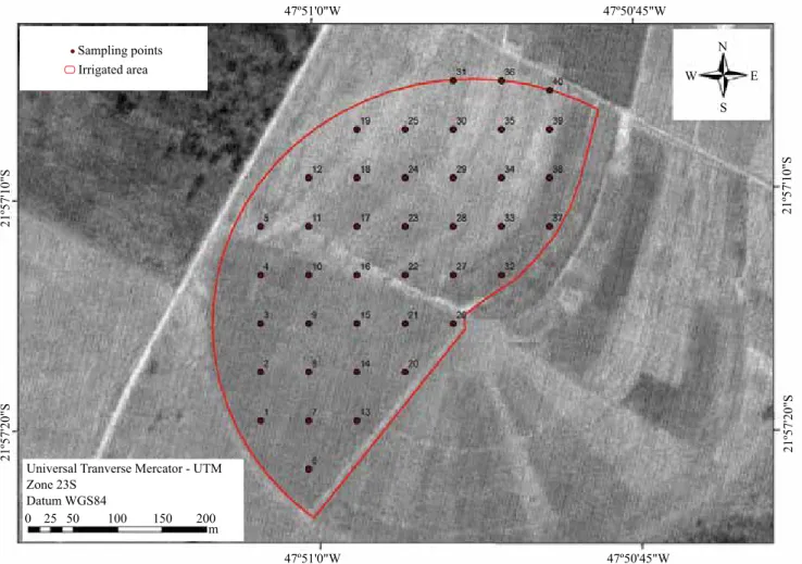
Sprinkler irrigation was performed by the center pivot irrigation system, and water management (amount
and frequency) was established based on the balance between climate demand (evapotranspiration) and the edaphic conditions (available water storage) of the site.
Only half of the irrigated area was cultivated with corn
(Figure 1).
The yield of irrigated corn for silage was evaluated between April and May 2011, 2012, and 2014 (years
1, 2, and 3 of the experiment), when the crop was
harvested at the dough stage, with dry matter between 28 and 35%. Biomass production was manually estimated in a regular grid of 40 georeferenced points
(Figure 1), representing 2.1 samples per hectare. In
each sampling point, 4.0-m length subsamples of corn aboveground biomass were collected from two lines to form a composite sample. Samples from the harvested material were taken to a forced-air circulation drying
Figure 1. Location and sampling points for yield evaluation of irrigated corn (Zea mays) crop for silage in the municipality
oven at 65ºC, until constant weight, for dry matter
determination.
The yield data of the three evaluated years were
subjected to the procedures of Blackmore (2000) and Molin (2002). The yield of each crop was normalized,
and the average yield per plot in the three crops was calculated; the percentage of this average was obtained for each sampling point. The standard deviation and
coefficient of variation (CV) were also calculated
for each sampling point, representing the temporal
variability of corn yield. From these values, yield was classified as: high, yield i > 105% yield average, CV < 30%; median, 95% ≤ yield I ≥ 105% yield average, CV < 30%; low, yield I < 95% yield average, CV < 30%; and inconsistent, CV ≥ 30%.
Based on the methodology proposed by Xu et al.
(2006), management classes were established for each
sampled point, considering the spatial (average yield
of each point) and temporal stability (CV) trends. Five
classes were taken into account in the present study: class 1, yield > yield average and CV <15%; class 2, yield
> yield average and 15% ≤ CVi <25%; class 3, yield <
yield average and CV <15%; class 4, yield < yield average and 15% ≤ CVi <25%; and class 5, CVi ≥ 25%.
Apparent soil EC was measured with the soil EC 3100 sensor (Veris Technologies, Salina, KS, USA).
The geographical coordinates of each measured point
were obtained with the GPSMAP 60CSx handheld GPS (Garmin International Inc., Olathe, KS, USA). By
May 2011, the equipment collected measurements at two different depths: 0.0–0.3 and 0.0–0.9 m.
The items and coefficients for production cost and profit simulations of the corn crop for silage were
obtained based on the spreadsheets of Tupy et al.
(2015). In this case, corn production costs considered: inputs, such as seeds, limestone, plaster, fertilizer,
and agricultural pesticides; machines, used for
pulverization, liming, plastering, sowing, fertilization,
and harvest; and labor, including planting, cultural
traits, harvest, and ensilage. Profit was calculated using
the reference system of milk production described by
Tupy et al. (2015), with Holstein cows producing an average of 25 kg milk per day, when feed: Tobiatã
grass [Megathyrsus maximus (Jacq.) B.K.Simon &
S.W.L.Jacobs] pasture, alfalfa (Medicago sativa L.),
and concentrated food in summer; and corn silage, alfalfa, and concentrated food in winter. The prices
were converted to American dollar at the quotation of
US$ 1.00 = R$3.417.
Data were assigned to the respective geo–coordinates
and exported to a GIS domain, the ArcGIS software,
version 10.1 (Environmental Systems Research
Institute, Redlands, CA, USA), as a shapefile for the
geostatistical analysis. Geostatistical analyses were performed for all variables in order to evaluate spatial dependence and continuity. The models of empirical omni-directional semivariograms were calculated
using the Vesper software (Oliveira, 2015), according
to the equation:
γ
h
N h
Z xi Z xi h
i N h
( )
=( )
= ( )
−(
+)
( )∑
1 2 2 1where Z(xi) and Z(xi + h) are the values observed for Z in the x and x + h location, respectively; h is the separation distance; and N(h) is the paired comparison number at an h distance. From the adjusted mathematical model, the following coefficients of the
semivariogram model, γ
( )
h , were calculated: nuggeteffect (C0), structural variance (C1), and reach (a). Contour maps were estimated by kriging using the Vesper software (Oliveira, 2015). The contour maps for each of the analyzed variables were obtained with
the ArcGIS software, version 10.1 (Environmental
Systems Research Institute, Redlands, CA, USA).
A 1,033-virtual sampling point grid was created in the GIS environment, and values of average yield,
normalized yield, management classes, production cost, profit, and apparent soil EC at the 0.0–0.3 and
0.0–0.9-m depths were obtained; then, Pearson’s correlations – tested by Student’s t-test, at 5.0, 1.0, and 0.1% probability – were established between them.
Results and Discussion
The yield data of the three evaluated years,
average and normalized yields, cost and profit
present asymmetry and kurtosis values compatible
with normality (Table 1), since theoretical values of asymmetry (<0.5) and kurtosis (<3.0) indicate normal distribution of data (Vian et al., 2016). The results of the
descriptive statistics indicated that all variables were
symmetric data, while the distribution of EC at 0.0–0.9 m (EC0.0-0.9) skewed to the right. This observation was
also supported by the closeness of mean and median
values (Table 1). In the geostatic analysis, normal
lead to more consistent results. Kriging also shows better results when data normality is satisfied (Grego & Oliveira, 2015). Average and normalized yields, as well as cost and profit, had a low CV (<10%). Yields in the three years of evaluation presented CVs considered medium (between 10 and 20%), while those of EC at 0.0–0.3 (EC0.0-0.3) and EC0.0-0.9 were high.
The experimental semivariograms were calculated,
and all adjusted models delimited for each year of
sampling (Table 2). The observations within the range of variogram (A) are considered spatially correlated
(Grego & Oliveira, 2015). Therefore, this range indicated the existence of spatial correlation for plant
and soil parameters over a long distance of >58 m and > 473 m, respectively. A sampling interval of less than half of the range of a variogram is recommended for
the adequate spatial characterization of parameters.
Therefore, a sampling distance shorter than 29 m can be used as a sampling interval for the spatial
characterization of parameters such as corn yield,
whereas a longer distance, i.e., a wider sampling
interval, of <237 m can be adopted for soil EC.
Table 1. Statistical parameters of average dry matter yield (DMY), normalized yield, management classes, production cost,
profit, and apparent soil electrical conductivity at the 0.0–0.3 (EC0.0-0.3) and 0.0–0.9-m (EC0.0-0.9) depths of irrigated corn
(Zea mays) crop for silage in the municipality of São Carlos, in the state of São Paulo, Brazil(1).
Variable Average Median Minimum Maximum SD Asymmetry Kurtosis CV (%) Number
DMY - Year 1 14,137 13,911 9,810 20,104 2,401 0.340 0.010 16.99 40
DMY - Year 2 13,897 13,996 9,419 18,543 1,929 0.069 0.121 13.88 40
DMY - Year 3 13,952 13,442 11,511 18,231 1,626 0.909 0.587 11.66 40
Average DMY (3 crops) 13,995 14,270 11,627 16,705 1,327 -0.072 -0.874 9.48 40
Normalized yield 99.51 101.85 83.08 115.25 9.484 -0.17 -1.05 9.11 40
Cost 102.50 100.14 85.64 122.91 9.947 0.39 -0.75 9.29 40
Profit 1,225.96 1,244.39 1,083.89 1,359.90 73.043 -0.31 -0.84 5.96 40
EC0.0-0.3 3.96 3.84 2.05 7.63 0.94 0.448 -0.341 23.8 14,815
EC0.0-0.9 5.53 4.79 1.90 19.01 2.65 1.784 4.340 48.0 14,793
(1)SD, standard deviation; and CV, coefficient of variation.
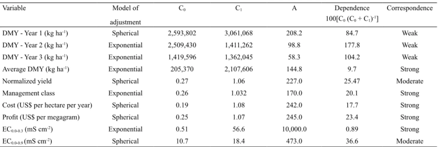
Table 2. Estimates of the parameters of the semivariogram models adjusted to average dry matter yield (DMY), normalized
yield, management classes, production cost, profit, and apparent soil electrical conductivity at the 0.0–0.3 (EC0.0-0.3) and
0.0–0.9-m (EC0.0-0.9) depths of irrigated corn (Zea mays) crop for silage in the municipality of São Carlos, in the state of São
Paulo, Brazil(1).
Variable Model of adjustment
C0 C1 A Dependence
100[C0 (C0 + C1)-1]
Correspondence
DMY - Year 1 (kg ha-1) Spherical 2,593,802 3,061,068 208.2 84.7 Weak
DMY - Year 2 (kg ha-1) Exponential 2,509,430 1,411,262 98.8 177.8 Weak
DMY - Year 3 (kg ha-1) Exponential 1,419,596 1,362,045 58.3 104.2 Weak
Average DMY (kg ha-1) Exponential 205,370 2,107,606 144.8 9.7 Strong
Normalized yield Spherical 0.27 1.06 227.0 25.47 Moderate
Management class Exponential 0.26 1.032 170.0 20.1 Strong
Cost (US$ per hectare per year) Spherical 0.19 1.08 242.0 17.7 Strong
Profit (US$ per megagram) Spherical 0.25 1.07 245.0 23.4 Strong
EC0.0-0.3 (mS cm-2) Exponential 0.51 56.6 10,000.0 0.89 Strong
EC0.0-0.9 (mS cm-2) Spherical 10.7 18.4 473.0 36.6 Moderate
(1)C
The exponential model was considered appropriate for the experimental variograms of years 2 and 3, average yield, management class, and EC0.0-0.3
parameters; however, for all others, the spherical
model stood out. The ratio between nugget effect (C0) and sill (C0 + C), expressed as percentage, was used
to determine the strength of the spatial dependence of
the studied parameters. These values characterize the random component of field data spatial variability and
also quantify the measurement of spatial dependence for the studied variables. The spatial dependencies
of the yields in the three experimental years can be considered weak, as they showed C0 above 76% of the threshold. Normalized yield and EC0.0-0.9 had moderate
dependencies between 25 and 75%, whereas average
yield, cost, profit, and EC0.0-0.3 presented strong dependencies, with C0 ≤ 25% of the threshold.
The obtained maps (Figure 2 A, B, and C) indicate
similarities among the three crops, grown in three
different years, i.e., seasons. However, the variation
in spatial distribution, considering average yield, is a steadier result, as already observed by Godwin et al.
(2003). Therefore, the average yield map (Figure 2 D)
shows the spatial trend for the period and reveals
that yield ranges may vary in approximately 39%, with greatest yield zones located in the northern and
northeastern regions of the map, and the lowest ones
in the central-west. Results from Vian et al. (2016) are
also indicative of the high spatial variability of corn yield even under irrigation.
Figure 2. Spatialized maps of dry matter yield of irrigated corn (Zea mays) crop for silage in the 2010 (A), 2011 (B), and
The averages of the sampling points for the three
analyzed crops were considered consistent, with CV>30%, indicating the repeatability of these values
throughout the sampled period and the consistency of the presented map, classifying the area into three
distinct management zones of low, medium, and high yield potential. The definition and spatialization of the management zones for this corn field allow identifying
the areas in which the yield of the system was similar
in the defined period (Figure 3 A).
A trend in spatial variability could be expected
for the three studied crops, as the chemical, physical and biological properties of the soil, essential for crop yield, can be relatively stable throughout time, despite
spatial variability (Joernsgaard & Halmoe, 2003). However, the differences observed across crop seasons
might derive from external factors, such as climate
and agricultural practices (Amado et al., 2009; Vian et
al., 2016), which can interact with soil properties and
create different patterns of crop yield variation from one year to the other.
Therefore, only establishing management zones
might not be enough for decision-making. Other
criteria may also be necessary, such as the coefficient of management (Blackmore, 2000; Xu et al., 2006),
which considers the spatial and temporal variability of yield. The map of management classes, based on
Blackmore (2000), is a synthesis of the spatial and
temporal stability trends of the three crop seasons
(Figure 3 B). Therefore, the maps obtained according to Blackmore (2000) and Molin (2002) can be an excellent
management tool and be adequately used for harvest estimation, since they are prepared considering the trend of different growing seasons, as recommended
by Rodrigues et al. (2013).
For average yield, a significant linear correlation coefficient was observed between normalized yield (0.99) and management class (-0.82) (Table 3). This result is essential, as it shows that both indexes allowed identifying differences in the assessed corn field.
The information from yield maps and management
zones is used to simplify spatial complexity, and the division of fields into subfields may support agronomic
management decisions (Rodrigues et al., 2013; Moshia
et al., 2014) as, for example, the optimization of the use of lime and fertilizer in areas of different yield
potential. Another strategy is the intervention in low
yield fields, with a more detailed diagnosis, followed
by a response based on the limiting factors detected.
However, the strategies for intervention in an area
depend on several factors such as land use history, adopted production system and agricultural practices,
and, as emphasized by Molin (2002), economic and financial aspects.
The production cost and profit (net income) maps incorporated the yield data of the three experimental
years and provided a scenario of the economic return
of the irrigated corn field (Figure 4 A and B). Three classes of production cost (US$ per megagram) were identified; the highest cost was on average 12 and 22% higher, respectively, than the average (US$ 98 to 111 per megagram) and low (US$ 85 to 98 per megagram) costs. Regarding profitability, differences of 6 to 12%
were observed between the class with the highest
Figure 3. Spatialized maps of normalized yield (A) and
below the limit. Moreover, the cost and net profit maps
translate yield data, which may be being collected by farmers for several years, as an understandable
Figure 4. Spatialized maps of the production cost (A) and
profit (B) of irrigated corn (Zea mays) crop for silage in the municipality of São Carlos, in the state of São Paulo, Brazil.
Figure 5. Spatialized maps of apparent soil electrical at the
0.0–0.3 (A) and 0.0–0.9-m (B) depths of irrigated corn (Zea mays) crop for silage in the municipality of São Carlos, in the state of São Paulo, Brazil.
Table 3. Pearson’s correlation coefficients between average yield, normalized yield, management classes, production cost,
profit, and apparent soil electrical conductivity (EC) at the 0.0–0.3 (EC0.0-0.3) and 0.0–0.9-m (EC0.0-0.9) depths of irrigated
corn (Zea mays) crop for silage in the municipality of São Carlos, in the state of São Paulo, Brazil.
Variable Normalized yield Management class Cost Profit EC0.0-0.3 EC0.0-0.9
Average yield 0.992*** -0.817** -0.975*** 0.993*** 0.529* 0.431*
Normalized yield -0.832** -0.962*** 0.995*** 0.533* 0.437*
Management class 0.776** -0.819** -0.526* -0.423*
Cost -0.971*** -0.524* -0.417*
Profit 0.434* 0.461*
EC0.0-0.3 0.451*
*, ** and ***Significant at 5.0, 1.0, and 0.1% probability, respectively.
economic return and the others. The cost and profit
estimates allow to establish economic benchmarks
feedback that can be directly applied to improve
site-specific management, as indicated by Massey et al. (2008). Significant correlation coefficients were found between corn yield and cost (r=-0.98***) and net profit (r=0.99***) (Table 3), confirming the importance of both
maps to aid farmers and technicians in interpreting
field variations and to support management decisions
(Blackmore, 2000; Blackmore et al., 2003; Rodrigues
et al., 2013).
Therefore, these results confirm that precision
agriculture can help both in the detection of limiting factors (Inamasu et al., 2011; Inamasu & Bernardi,
2014) and in decision making regarding site-specific management strategies to improve crop profitability
(Xu et al., 2006; Massey et al., 2008; Bernardi et al.,
2016; Verruma et al., 2017).
The zones that need particular attention were identified in the present study and could be treated by specific measures. Therefore, it is recommended that
limiting factors be diagnosed and, whenever possible, corrected before the application of spatially variable issues.
The spatial distribution of the soil EC evaluated at two different soil depths (EC0.0-0.30 and EC0.0-0.90)
showed spatial patterns similar to those of corn yield
(Figure 5 A and B). The shallow depth of 0.0–0.3 m presented EC values between 1.8 and 12 dS m-1, and
the deeper one of 0.0–0.9 m, between 0.5 and 44 dS m-1. As the EC value is positively influenced by soil clay content (Johnson et al., 2005; Machado et al., 2006), the regions with higher EC reflect the quantity of clay (Moral et al., 2010). Consequently, regions with
high clay typically indicate soil with a high organic
matter content, cation exchange capacity, and available
ions to the soil solution, conditions that increase soil
yield potential. Corroborating the previous findings of Johnson et al. (2005) and Moral et al. (2010), average and normalized yields, as well as management class maps, were significantly related to the soil EC0.0-0.3 and EC0.0-0.9 values (Table 3) measured by the Veris sensor (Veris Technologies, Salina, KS, USA).
Conclusions
1. There is a structured spatial variability of corn (Zea mays) yield, production cost, profit, and soil
electrical conductivity within the irrigated area.
2. The evaluated precision agriculture tools are
useful to indicate zones of higher yield and economic
return.
3. The sequences of yield maps and the analysis of
spatial and temporal variability allow the definition of management zones.
References
ACOMPANHAMENTO DA SAFRA BRASILEIRA [DE] GRÃOS: Safra 2017-18. 2018. Available at: <http://www.conab. gov.br/OlalaCMS/uploads/arquivos/18_02_08_17_09_36_ fevereiro_2018.pdf>. Accessed on: Feb. 28 2018.
ALBA, J.M.F. Modelagem SIG em agricultura de precisão: conceitos, revisão e aplicações. In: BERNARDI, A.C. de C.; NAIME, J. de M.; RESENDE, A.V. de; BASSOI, L.H.; INAMASU, R.Y. (Ed.). Agricultura de precisão: resultados de um novo olhar. Brasília: Embrapa, 2014. p.84-96.
AMADO, T.J.C.; PES, L.Z.; LEMAINSKI, C.L.; SCHENATO, R.B. Atributos químicos e físicos de Latossolos e sua relação com os rendimentos de milho e feijão irrigados. Revista Brasileira de Ciência do Solo, v.33, p.831-843, 2009. DOI: 10.1590/S0100-06832009000400008.
AMADO, T.J.C.; PONTELLI, C.B.; SANTI, A.L.; VIANA, J.H.M.; SULZBACH, L.A. de S. Variabilidade espacial e temporal
da produtividade de culturas sob sistema plantio direto. Pesquisa Agropecuária Brasileira, v.42, p.1101-1110, 2007. DOI: 10.1590/ S0100-204X2007000800006.
BERNARDI, A.C.C.; BETTIOL, G.M.; FERREIRA, R.P.; SANTOS, K.E.L.; RABELLO, L.M.; INAMASU, R.Y. Spatial variability of soil properties and yield of a grazed alfalfa pasture in Brazil. Precision Agriculture, v.17, p.737-752, 2016. DOI: 10.1007/ s11119-016-9446-9.
BLACKMORE, S. The interpretation of trends from multiple yield
maps. Computers and Electronics in Agriculture, v.26, p.37-51,
2000. DOI: 10.1016/S0168-1699(99)00075-7.
BLACKMORE, S.; GODWIN, R.J.; FOUNTAS, S. The analysis of spatial and temporal trends in yield map data over six years.
Biosystems Engineering, v.84, p.455-466, 2003. DOI: 10.1016/
S1537-5110(03)00038-2.
CALDERANO FILHO, B.; SANTOS, H.G. dos; FONSECA, O.O.M. da; SANTOS, R.D. dos; PRIMAVESI, O.; PRIMAVESI, A.C. Os solos da fazenda Canchim, Centro de Pesquisa de Pecuária do Sudeste, São Carlos, SPP: levantamento semidetalhado,
propriedades e potenciais. Rio de Janeiro: Embrapa-CNPS; São Carlos: Embrapa-CPPSE, 1998. 95p. (Embrapa-CNPS. Boletim de Pesquisa, 7; Embrapa-CPPSE. Boletim de Pesquisa, 2).
DOERGE, T. Defining management zones for precision farming.
Crop Insights, v.8, p.1-5, 1999.
GEBBERS, R.; ADAMCHUK, V.I. Precision agriculture and
food security. Science, v.327, p.828-831, 2010. DOI: 10.1126/ science.1183899.
GODWIN, R.J.; MILLER, P.C.H. A review of the technologies for mapping within-field variability. Biosystems Engineering, v.84,
p.393-407, 2003. DOI: 10.1016/S1537-5110(02)00283-0.
GREGO, C.R.; OLIVEIRA, R.P. de. Conceitos básicos da Geoestatística. In: OLIVEIRA, R.P. de; GREGO, C.R.; BRANDAO, Z.N. (Ed.). Geoestatística aplicada na agricultura de precisão utilizando o Vesper. Brasília: Embrapa, 2015. p.41-62.
INAMASU, R.Y.; BERNARDI, A.C. de C. Agricultura de precisão. In: BERNARDI, A.C. de C.; NAIME, J. de M.; RESENDE, A.V. de; BASSOI, L.H.; INAMASU, R.Y. (Ed.). Agricultura de precisão: resultados de um novo olhar. Brasília: Embrapa, 2014. p.21-33.
INAMASU, R.Y.; BERNARDI, A.C. de C.; VAZ, C.M.P.; NAIME, J. de M.; QUEIROS, L.R.; RESENDE, A.V. de; VILELA, M. de F.; JORGE, L.A. de C.; BASSOI, L.H.; PEREZ, N.B.; FRAGALLE, E.P. Agricultura de precisão para a sustentabilidade de sistemas produtivos do agronegócio brasileiro. In: INAMASU, R.Y.; NAIME, J.M.; RESENDE, A.V.; BASSOI, L.H.; BERNARDI, A.C.C. (Ed.). Agricultura de precisão: um novo olhar. São Carlos:
Embrapa Instrumentação, 2011. p.14-26.
JOERNSGAARD, B.; HALMOE, S. Intra-field yield variation over
crops and years. European Journal of Agronomy, v.19, p.23-33,
2003. DOI: 10.1016/S1161-0301(02)00016-3.
JOHNSON, C.K.; ESKRIDGE, K.M.; CORWIN, D.L. Apparent
soil electrical conductivity: applications for designing and
evaluating field-scale experiments. Computers and Electronics in Agriculture, v.46, p.181-202, 2005. DOI: 10.1016/j. compag.2004.12.001.
MACHADO, P.L.O. de A.; BERNARDI, A.C. de C.; VALENCIA, L.I.O.; MOLIN, J.P.; GIMENEZ, L.M.; SILVA, C.A.; ANDRADE, A.G. de; MADARI, B.E.; MEIRELLES, M.S.P. Mapeamento da condutividade elétrica e relação com a argila de Latossolo sob
plantio direto. Pesquisa Agropecuária Brasileira, v.41, p.1023-1031, 2006. DOI: 10.1590/S0100-204X2006000600019.
MASSEY, R.E.; MYERS, D.B.; KITCHEN, N.R.; SUDDUTH, K.A. Profitability maps as an input for site-specific management
decision making. Agronomy Journal, v.100, p.52-59, 2008. DOI: 10.2134/agronj2007.0057.
MOLIN, J.P. Definição de unidades de manejo a partir de mapas de
produtividade. Engenharia Agrícola, v.22, p.83-92, 2002.
MORAL, F.J.; TERRÓN, J.M.; SILVA, J.R.M. da. Delineation of management zones using mobile measurements of soil apparent
electrical conductivity and multivariate geostatistical techniques.
Soil and Tillage Research, v.106, p.335-343, 2010. DOI: 10.1016/j. still.2009.12.002.
MOSHIA, M.E.; KHOSLA, R.; LONGCHAMPS, L.; REICH, R.; DAVIS, J.G.; WESTFALL, D.G. Precision manure management across site-specific management zones: grain yield and economic
analysis. Agronomy Journal, v.106, p.2146-2156, 2014. DOI: 10.2134/agronj13.0400.
OLIVEIRA, R.P. de. O Vesper. In: OLIVEIRA, R.P. de; GREGO, C.R.; BRANDAO, Z.N. (Ed.). Geoestatística aplicada na agricultura de precisão utilizando o Vesper. Brasília: Embrapa, 2015. p.65-82.
RODRIGUES, M.S.; CORÁ, J.E.; CASTRIGNANÒ, A.; MUELLER, T.G.; RIENZI, E. A spatial and temporal prediction
model of corn grain yield as a function of soil attributes. Agronomy Journal, v.105, p.1878-1887, 2013. DOI: 10.2134/agronj2012.0456.
SANTI, A.L.; AMADO, T.J.C.; EITELWEIN, M.T.; CHERUBIN, M.R.; SILVA, R.F. da; DA ROS, C.O. Definição de zonas de produtividade em áreas manejadas com agricultura de precisão.
Revista Brasileira de Ciências Agrárias, v.8, p.510-515, 2013. DOI: 10.5039/agraria.v8i3a2489.
TUPY, O.; FERREIRA, R. de P.; VILELA, D.; ESTEVES, S.N.; KUWAHARA. F.A.; ALVES, E.A. Viabilidade econômica e financeira do pastejo em alfafa em sistemas de produção de leite.
Revista de Política Agrícola, ano 24, p.102-116, 2015.
VERRUMA, A.A.; MARTINELLI, P.R.P.; RABELLO, L.M.; INAMASU, R.Y.; SANTOS, K.E.L.; BETTIOL, G.M.; BERNARDI, A.C.C. Soil and weed occurrence mapping and
estimates of sugarcane production cost. Brazilian Journal of Biosystems Engineering, v.11, p.68-78, 2017.
VIAN, A.L.; SANTI, A.L.; AMADO, T.J.C.; CHERUBIN, M.R.; SIMON, D.H.; DAMIAN, J.M.; BREDEMEIER, C. Variabilidade espacial da produtividade de milho irrigado e sua correlação com variáveis explicativas de planta. Ciência Rural, v.46, p.464-471, 2016. DOI: 10.1590/0103-8478cr20150539.
XU, H.-W.; WANG, K.; BAILEY, J.S.; JORDAN, C.; WITHERS,
A. Temporal stability of sward dry matter and nitrogen yield patterns in a temperate grassland. Pedosphere, v.16, p.735-744,
2006. DOI: 10.1016/S1002-0160(06)60109-4.