Patrícia Justo Bota
Bachelor Degree in Biomedical Engineering Sciences
Human Activity Annotation based on Active
Learning
Dissertation submitted in partial fulfillment of the requirements for the degree of
Master of Science in Biomedical Engineering
Adviser: Prof. Dr. Hugo Filipe Silveira Gamboa, Professor Auxiliar, Faculdade de Ciências e Tecnologias, Universidade Nova de Lisboa
Examination Committee
Chairperson: Prof. Dr. Carla Maria Quintão Pereira
Human Activity Annotation based on Active Learning
Copyright © Patrícia Justo Bota, Faculty of Sciences and Technology, NOVA University Lisbon.
The Faculty of Sciences and Technology and the NOVA University Lisbon have the right, perpetual and without geographical boundaries, to file and publish this dissertation through printed copies reproduced on paper or on digital form, or by any other means known or that may be invented, and to disseminate through scientific repositories and admit its copying and distribution for non-commercial, educational or research purposes, as long as credit is given to the author and editor.
Ac k n o w l e d g e m e n t s
First and foremost, I would like to express my utmost gratitude to my academic super-visor Prof. Hugo Gamboa, for giving me the opportunity to enter the world of machine learning and data science. Thank you for all the insights and excellent advice during the development of this dissertation.
I would like to thankAssociação Fraunhofer Portugal Researchfor the opportunity to
work on my thesis in such a good environment, where I was encouraged to always, think, learn and dare. Especially, I would like to thank Duarte Folgado and Joana Silva, for the guidance, support and promptly help, that allowed me to learn everyday and successfully complete this research with great enthusiasm.
Thank you to all my university friends and my colleagues at Fraunhofer, for being a great influence in my life, and for all the laughs and silly moments that made all the study and stress times easier.
A b s t r a c t
Human activity recognition algorithms have been increasingly sought due to their broad application, in areas such as healthcare, safety and sports. Current works focusing on human activity recognition are based majorly on Supervised Learning algorithms and have achieved promising results. However, high performance is achieved at the cost of a large amount of labelled data required to train and learn the model parameters, where a high volume of data will increase the algorithm’s performance and the classifier’s ability to generalise correctly into new, and previously unseen data. Commonly, the labelling process of ground truth data, which is required for supervised algorithms, must be done
manually by the user, being tedious, time-consuming and difficult.
On this account, we propose a Semi-Supervised Active Learning technique able to partly automate the labelling process and reduce considerably the labelling cost and the labelled data volume required to obtain a highly performing classifier. This is achieved through the selection of the most relevant samples for annotation and propagation of their label to similar samples. In order to accomplish this task, several sample selection strategies were tested in order to find the most valuable sample for labelling to be in-cluded in the classifier’s training set and create a representative set of the entire dataset. Followed by a semi-supervised stage, labelling with high confidence unlabelled samples,
and augmenting the training set without any extra labelling effort from the user. Lastly,
five stopping criteria were tested, optimising the trade-offbetween the classifier’s
perfor-mance and the percentage of labelled data in its training set.
Experimental results were performed on two different datasets with real data,
allow-ing to validate the proposed method and compare it to literature methods, which were replicated. The developed model was able to reach similar accuracy values as supervised learning, with a reduction in the required labelled data of more than 89% for the two datasets, respectively.
Keywords: Human Activity Recognition, Machine Learning, Feature Selection, Active
R e s u m o
Os algoritmos de reconhecimento de atividade humana têm sido cada vez mais procu-rados devido à sua grande aplicabilidade, em áreas como a saúde, segurança e desporto. As soluções existentes são baseadas, principalmente, em algoritmos de Aprendizagem Supervisionada atingindo resultados promissores. Porém, requerendo uma grande quan-tidade de dados anotados, necessários para treinar e aprender os parâmetros do modelo. Esta anotação, dado que deve ser realizada manualmente pelo utilizador, é um processo fastidioso, demorado e difícil.
Assim, esta tese propõe uma técnica envolvendo métodos de Aprendizagem Ativa Semi-Supervisionada, capaz de automatizar parcialmente o processo de anotação através da seleção da amostra considerada como mais relevante para a classificação e propa-gando a sua etiqueta a amostras semelhantes. Deste modo, reduzindo significativamente o esforço manual por parte do utilizador na anotação. Para isto, foram testadas várias estratégias para a seleção da amostra para anotar e incorporar no conjunto de treino do classificador. Adicionalmente, foi introduzido um estado Semi-Supervisionado, permi-tindo uma anotação automática de amostras não anotadas e, assim, aumentar o conjunto de treino do classificador sem qualquer esforço por parte do utilizador. Por último, cinco critérios de paragem para o algoritmo realizado foram testados, tendo como objetivo oti-mizar o balanço entre o desempenho do classificador e a percentagem de dados anotados existentes no seu conjunto de treino.
Testes experimentais foram realizados em dois conjuntos de dados reais, permitindo validar o método proposto e compará-lo a métodos já existentes, que foram replicados. Nos resultados obtidos foi obtida uma precisão semelhante a alcançada pela técnica supervisionada, com uma redução na quantidade de dados anotados de 89%, para ambos os conjuntos de dados.
Palavras-chave: Reconhecimento de Atividade Humana, Aprendizagem Automática,
C o n t e n t s
List of Figures xiii
List of Tables xv
Acronyms xix
1 Introduction 1
1.1 Motivation . . . 1
1.2 Objectives . . . 4
1.3 State of the Art . . . 5
1.4 Thesis Overview . . . 8
2 Theoretical Background 9 2.1 Wearable and Smartphone Sensors . . . 9
2.1.1 Accelerometer . . . 9
2.1.2 Gyroscope . . . 11
2.1.3 Barometer . . . 12
2.2 Machine Learning . . . 13
2.2.1 Signal Processing . . . 13
2.2.2 Feature Engineering . . . 14
2.2.3 Classification . . . 15
2.2.4 Validation . . . 25
3 Framework for Human Activity annotation based on Active Learning 27 3.1 Signal Acquisition and Processing . . . 27
3.2 Feature Engineering . . . 28
3.3 General Active Learning Strategy . . . 30
3.3.1 Initial Train Set . . . 31
3.3.2 Sample Selection Strategy . . . 31
3.3.3 Stopping Criterion . . . 36
3.4 Semi-Supervised Active Learning Framework . . . 39
3.4.1 Similarity Measures . . . 41
CO N T E N T S
4 Results 47
4.1 Datasets . . . 47
4.2 Feature Extraction and Selection . . . 48
4.3 Model Selection . . . 49
4.4 Query Strategy Analysis . . . 49
4.5 Active Learning Semi-Supervised Analysis . . . 55
4.6 Stopping Criterion Analysis . . . 59
5 Conclusion 65 5.1 Overall Achievements . . . 65
5.2 Future Work . . . 68
Bibliography 69
A Acquisition Devices 75
B Algorithms 77
L i s t o f F i g u r e s
1.1 Demonstration of the working principles of AL and SSAL. . . 4
1.2 Thesis overview structure. . . 8
2.1 Smartphone’s sensors standard coordinate system and accelerometer sensor output signal with the device positioned into different orientations. . . . 10
2.2 Smartphone’s sensors standard coordinate system and gyroscope’s output sig-nal with the device positioned into different orientations. . . . 11
2.3 Barometer’s output signal from a user climbing up and downstairs. . . 12
2.4 Accelerometer’s signal magnitude of the total and body accelerations. . . 13
2.5 Pipeline description ofSupervised Learning. . . 15
2.6 Pool-basedActive Learningcycle. . . 21
2.7 Active Learning training set samples two-dimensional principal component analysis. . . 22
2.8 Active Learning UCI test set samples two-dimensional principal component analysis. . . 22
2.9 Self-Trainingtraining set samples two-dimensional principal component anal-ysis. . . 24
2.10 Self-TrainingUCI test set samples two-dimensional principal component anal-ysis. . . 24
3.1 Schematic representation of the framework developed in this thesis. . . 27
3.2 Accelerometer’s signal before and after the application of a band-pass filter. 29 3.3 Computation of the uncertainty score according toLeast Confident Sampling. 32 3.4 Computation of the uncertainty score according toMargin Sampling. . . 33
3.5 Computation of the uncertainty score according toEntropy Sampling. . . 34
3.6 UCI samples’ information density on a two-dimensional principal component analysis. . . 35
3.7 Active Learningperformance curve throughout 300 iterations. . . 37
3.8 Classifier Least Confidence score and Classifier Overall Uncertainty score throughout 300 iterations. . . 37
3.9 Example of 1-Nearest Neighbourlabel propagation step. . . 40
L i s t o f F i g u r e s
3.11 Two-dimensional illustration of theEuclidean distanceand theCosine similarity
between two samples. . . 42
3.12 Comparison between theEuclidean DistanceandDynamic Time Warping
Dis-tancebetween two signals. . . 44
4.1 Classifier’s accuracy score during and beforeForward Feature Selection. . . 49
4.2 Active Learningclassifier’s accuracy for the different developed query strategies. 52
4.3 Principal component analysis of the Active Learning training set and Local
Density * Margin Samplinguncertainty score heatmap. . . 52
4.4 Principal component analysis of theActive Learningtraining set using theLeast
Confident Samplingand theLocal Density * Least Confident Sampling. . . 53 4.5 Local Density * Least Confident SamplingandMargin Samplinguncertainty score
heatmaps. . . 54
4.6 Classifier’s accuracy for the developedSemi-Supervised Active Learning
meth-ods throughout the cycle iterations. . . 56
4.7 Percentage of the validation set unlabelled samples for the developed
Semi-Supervised Active Learningmethods throughout theActive Learningiterations. 57 4.8 Percentage of correctly automatically annotated samples for the developed
Semi-Supervised Active Learningmethods throughout theActive Learning iter-ations. . . 57
4.9 Horizon Plot for the misclassified activities . . . 60
4.10 Confusion matrix for theST-SSALmethod using theOverall Uncertainty SC. . 61
A.1 CADL dataset acquisition devices. . . 75
A.2 Percentage of samples belonging to each performed activity for the UCI and
CADL datasets. . . 76
C.1 Horizon Plot for the UCI dataset, allowing to visualise the behaviour of the
best features set along the protocol activities. . . 82
C.2 Horizon Plot for the CADL dataset, allowing to visualise the behaviour of the
L i s t o f Ta b l e s
1.1 Sources of labelled data with a brief description, main advantages and
disad-vantages. . . 3
2.1 Statistical, Temporal and Spectral Domain Features used in the present work. 16 2.2 Common distance metrics and their math formula. . . 17
2.3 Illustration of a Confusion Matrix. . . 26
2.4 Evaluation metrics for a binary classification. . . 26
4.1 Summary information on UCI and CADL dataset. . . 48
4.2 SL and UL methods classification’s performance shown in accuracy and ARI score, respectively. . . 50
4.3 Active Learningexperimental results for the developed query strategies. . . . 50
4.4 Active Learningexperimental results for the developed query strategies. . . . 51
4.5 Experimental results for the SSAL methods. . . 62
L i s t o f A l g o r i t h m s
1 Filtering . . . 28
2 Feature Extraction . . . 29
3 Forward Feature Selection . . . 30
4 General Active Learning . . . 31
5 General Semi-Supervised Active Learning . . . 39
6 K-fold Cross Validation . . . 45
7 Active Learning Applying The Max-Confidence SC . . . 77
8 Active Learning Applying The Overall Uncertainty SC . . . 78
9 Active Learning Applying The Classification-Change SC . . . 78
10 Active Learning Applying The Combination Strategy SC . . . 78
11 Self-Training . . . 79
12 5-Nearest Neighbour Semi-Supervised Active Learning . . . 79
Ac r o n y m s
AICOS Assistive Information and Communication Solutions.
AL Active Learning.
Ann Acc Automated Annotation Accuracy.
ARI Adjusted Rand Index.
Aut Ann Automated Annotation Percentage.
CADL Continuous Activities of Daily Living.
CC Classification-Change.
CV Cross Validation.
DBSCAN Density-Based Spatial Clustering of Applications with Noise.
DTW Dynamic Time Warping.
FN False Negative.
FP False Positive.
HAR Human Activity Recognition.
Max-CC Max-Confidence Uncertainty and Classification-Change.
Max-Conf Max-Confidence.
MEMS Micro-Electro-Mechanical-Systems.
NN Nearest Neighbour.
Over-CC Overall Uncertainty and Classification-Change.
Over-Unc Overall Uncertainty.
PCA Principal Component Analysis.
AC R O N Y M S
QDA Quadratic Discriminant Analysis.
QS Query Strategy.
QSs Query Strategies.
rNN Reverse-Nearest Neighbour.
SC Stopping Criterion.
SCs Stopping Criteria.
SL Supervised Learning.
SP Stopping Point.
SSAL Semi-Supervised Active Learning.
SSL Semi-Supervised Learning.
ST Self-Training.
SVM Support Vector Machine.
TAM Time Alignment Metric.
TN True Negative.
TP True Positive.
UCI University of California, Irvine.
C
h
a
p
t
e
r
1
I n t r o d u c t i o n
1.1 Motivation
Over the last years, the technological advances on ubiquitous sensing mechanisms allow the proliferation of available data, which often is unlabelled. Modern machine learning approaches require large amounts of labelled data to achieve adequate performance. This duality raises a relevant question: How can we simultaneously optimise the process of data annotation and still learn an accurate machine learning model?
Particularly, the HAR field has been a source of large quantity of available data, mostly due to its myriad of applications on real-life scenarios such as healthcare, indoor location, user-adaptive recommendations and transportation [1, 2]. According to the World Health
Organisation [3], insufficient physical activity has been identified as the fourth leading
risk factor for global mortality. Indeed, physical inactivity is one of the main causes of several health diseases, being correlated with overweight and obesity. On the other hand, the practice of physical exercise is correlated to an increase of cardio-respiratory and muscular fitness, functional health, cognitive functions and improvement of bones and joint health. As a result, human physical activities recognition has been increasingly sought in a personal fitness tracking context, giving the necessary motivation to physical activities practice.
Alongside withhealthcare, the monitoring of the human movement can be paramount
as a preventive and diagnosis tool, contributing to its usersafetyby the identification
of psychiatric disorders signs, and warnings of unusual activity, such as falls, movement degeneration or cardiac abnormalities.
Likewise, in aphysiotherapyorsportssetting, monitoring the body movements can
C H A P T E R 1 . I N T R O D U C T I O N
data information and motivation for improvement.
Besides these concerns, Human Activity Recognition (HAR) can be a powerful tool in
smart homes, allowing to interpret the current user state so the house system can better
reply to the user’s needs. As well forindoor locationsystems, where the GPS is often
not available. Moreover, since many activities are location dependent, the recognition of human movement activities can be helpful to infer the user’s position.
For this reason, human physical activity monitoring has been increasingly sought by physicians, athletes, physiotherapists, researchers and even healthy individuals, wanting to maintain and improve their healthy, active lifestyle [4].
Under those circumstances, HAR has been the subject for numerous studies, with the major part based on Supervised Learning (SL) machine learning techniques [4–6]. These have achieved great results, however, at the cost of involving the collection of large amounts of labelled data. Where a high volume of data will increase the algorithm’s performance and the classifier’s ability to generalise correctly into new, unseen data.
Moreover, data does not get labelled automatically but through a labelling process,
also referred to asannotation, where each unlabelled sample is mapped into a label. Thus,
becoming what is denoted aslabelled data. Furthermore, most of the times, the
annota-tion must be performed manually by the user, being time-consuming, difficult, or even
impossible to obtain, as it there can be no means to know the samples’ labels. Therefore, this fact highly limits a real-life application of today’s approaches and their scalability. In fact, generally, behind every classifier training set, there are timeless, arduous hours of annotation usually performed manually by a human worker. Per example, ImageNet, an image database, had for 9 years, contributors manually annotating more than 14 million images [7]. A process that will be the core of any classifier using the database, where
any mistake, per example, annotating a cat as a dog, will affect greatly the classifier’s
quality and its results. Therefore, most of the time, the developer’s time is not spent on building the classifier, but on acquiring data and annotating it, in order to be able to create a highly confident classifier. Indeed, annotating a dataset is not only time costly
and difficult, but also extremely expensive for a company. For instance, annotating the
Cityscapes dataset1, containing stereo video sequences with a total of 5000 high-quality
pixel level annotated frames and, considering that annotating a single image can take around at least 1.5h. Annotating the entire dataset would require a total of 5000 * 1.5 =
7500h. Thus, taking into account that 1 hour approximately costs 4e (approximately the
minimum wage by the hour in Portugal [8]) that would make a total cost of 30 000e.
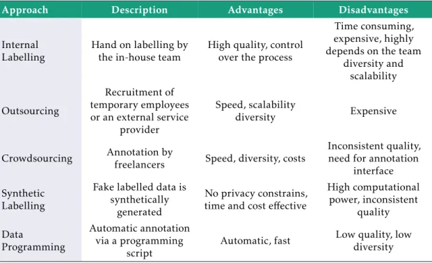
Table 1.1 enumerates some of the most common sources for training data. As it can be observed, there is not one to stand out as ideal [7]. Therefore, under those circumstances, the development of a new method able to partly automate the annotation process, and reduce considerably its expensive cost is challenging and particularly interesting.
1 . 1 . M O T I VAT I O N
Table 1.1: Sources of labelled data with a brief description, main advantages and disad-vantages.
Approach Description Advantages Disadvantages
Internal Labelling
Hand on labelling by the in-house team
High quality, control over the process
Time consuming, expensive, highly depends on the team
diversity and scalability
Outsourcing
Recruitment of temporary employees or an external service
provider
Speed, scalability
diversity Expensive
Crowdsourcing Annotation by
freelancers Speed, diversity, costs
Inconsistent quality, need for annotation
interface Synthetic
Labelling
Fake labelled data is synthetically
generated
No privacy constrains, time and cost effective
High computational power, inconsistent quality Data Programming Automatic annotation via a programming
script
Automatic, fast Low quality, low diversity
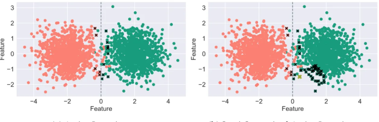
In datasets with significant size, not all samples are equally informative to the clas-sification process and an arbitrary unlabelled example may even be redundant. Active Learning (AL) provides methods to automatically identify the most relevant samples, which are posteriorly queued for expert annotation, that we denote as Oracle, without compromising the model performance. Figure 1.1a, illustrates the behaviour of AL where samples near the decision boundary are denoted as more informative, therefore, are se-lected for annotation. Additionally, Figure 1.1b displays the Semi-Supervised Active Learning automatic annotation behaviour where after the most informative sample se-lected by AL (in yellow) is annotated by the oracle, its nearest samples are automatically
annotated (as shown by the×in black).
In this dissertation, we apply a SSAL algorithm for HAR, where we establish criteria to select the most relevant samples for annotation and propagate their label to similar samples. Moreover, the model is created with a minimal initial training set and a com-prehensive study regarding state of art AL Query Strategies (QSs), Stopping Criteria (SCs) and distance functions was performed. The SSAL method based on Self-Training (ST) applied to HAR data, starting with near zero annotated data, achieved high results
on algorithm’s performance while reducing considerably the annotation effort and
C H A P T E R 1 . I N T R O D U C T I O N
−4 −2 0 2 4
Feature −2
−1 0 1 2 3
Fe
at
ure
(a) Active Learning.
−4 −2 0 2 4
Feature −2
−1 0 1 2 3
Fe
at
ure
(b) Semi-Supervised Active Learning.
Figure 1.1: A dataset of 3000 samples illustrating the working principles of AL and Semi-Supervised Active Learning (SSAL). The samples are illustrated with colours identifying their respective class. The samples selected by the AL for expert annotation are depicted
by the×’s. The grey vertical line denotes the decision boundary between the two classes.
1.2 Objectives
This dissertation was developed in collaboration with Fraunhofer Assistive Information and Communication Solutions (AICOS) Portugal. This research centre focuses on creating ’Remarkable Technology, Easy to Use’, developing tomorrow’s technologies contributing to economic growth, social well-being and an improved quality of life of its end users [9].
Moreover, this thesis focuses on the development of a framework for HAR with mi-nor annotation cost for the user, using the smartphone and wearable devices’ sensors. Furthermore, this dissertation proposes to infer how much labelled data it is required to train and create a model able to reach a highly confident classification performance as the obtained by SL techniques.
In order to perform this task, two major approaches will be followed: the first based
onAL, exploring several Query Strategy allowing to select highly informative samples to
annotate and integrate into the classifier’s training set. Followed by a second framework,
combining bothALand aSemi-Supervised Learningstep, aiming to, through the later,
to automatically label additional unlabelled data with no annotation effort for the user.
Thus, to develop the above-mentioned frameworks, the following steps, describing the core components of any HAR system, must be implemented:
1. Signal Acquisition and Extraction:acquisition and extraction of the smartphone
and the wearable devices sensors signals. Analysis of the required number of de-vices, their position and orientation, and the number and type of sensors to use.
2. Signal Processing:signal segmentation and filtering. Analysis of the type of sliding
window, dimension, type of filters, and cutofffrequencies.
3. Feature Engineering:feature extraction and selection on statistical, temporal and
1 . 3 . S TAT E O F T H E A R T
4. Active Learning and Semi-Supervised Active Learning Framework:development
of a framework to recognise human motion activities requiring minimal annotation cost.
5. Frameworks’ Optimisation:study of the selective sampling QSs and the AL
stop-ping criteria.
6. Performance Evaluation:evaluation of the developed algorithms.
1.3 State of the Art
In the literature, the discrimination of human activities is often covered by external or wearable sensors. The former include intelligent homes, where sensors are placed in critical devices and cameras. However, these raise numerous issues, such as privacy, pervasiveness and complexity concerns [2, 6]. Thus, motivating the use of wearable sensors, since their small size, low cost and non-obtrusiveness allow to integrate them easily into the users’ daily living activities.
On this account, many wearable sensor-based Machine Learning classification tech-niques have surged, namely, SL techtech-niques. As in the work of Silva [4], where the author used the smartphone accelerometer data, obtained using the acquisition device located on the user’s waist, to train and classify a decision tree algorithm. Moreover, feature extraction and selection methods were applied to the signal, reducing significantly the algorithm time and computational complexity. In the final result, the classifier obtained a total accuracy of 86%. Thus, it was possible to conclude that, with a smartphone, it is possible to retrieve the users’ activity data with good results and great comfort for the user.
Additionally, in order to overcome the implications of a pre-defined fixed device position, Figueira [5] developed a framework to perform HAR independently of the user and the device position in relation to the user’s body. To perform this task a decision tree algorithm was implemented and obtained an accuracy of 94.6% using accelerometer and barometer data. The addition of the barometer data, measuring the ambient air pressure, shown to be especially important in the recognition of vertical movements, such as climbing and descending stairs.
However, these works used SL techniques, and therefore, require the entire classifier’s
training set to be previously annotated: a costly, difficult and time-consuming task as
described in Section 1.1. On this account, in order to minimise the classifier’s training
set high annotation cost, we propose the use of anALbased methodology to recognise
simple daily living activities. Furthermore, an AL System is composed by two main parts:
the Query System that selects the relevant samples to be annotated and incorporated
C H A P T E R 1 . I N T R O D U C T I O N
In the literature, several techniques for the query system have been proposed.
How-ever, regarding HAR, they majorly follow aQuery by CommitteeorPool Samplingstrategy
[10, 11].
Henceforth, in aQuery by Committee Sampling, a committee of classifiers is created
as a voting system for the label of each sample, so that in every iteration, the sample with
the highest label disagreement between the different classifiers is selected as the most
informative for the oracle to annotate.
On the other hand, inPool-based Sampling, the unlabelled samples create a pool
from which the learner selects the most informative sample for the oracle to annotate according to a pre-defined score [11–14].
With this in mind, Shahmohammadi et al. [10] applied both theQuery by Committee
and thePool-based Sampling query systems in a smartwatch-based approach dedicated
to HAR. The two approaches surpassedRandom Sampling(where a sample is randomly
selected from the unlabelled samples dataset), withPool-based Samplingobtaining the
best results. Moreover, generally speaking, the proposed method was able to achieve an accuracy of 92%, with a reduction of 46% in the amount of annotated data in comparison to SL. Therefore, proving the application of AL in the context of HAR and its ability to significantly reduce the required amount of labelled data.
Similarly, Rong Liu et al. [11] applied an AL novel method in the context of HAR using body-worn accelerometer sensor data. In the developed algorithm two QSs were
implemented and in both the accuracy was higher than in Random Sampling. The first,
entitled a Pool-based SamplingQuery Strategy (QS) based on the classifier’s prediction
confidence. While the second followed a Query by Committee Sampling QS using two
classifiers trained on the hip and wrist devices’ data, respectively. The proposed method was evaluated with initial train sets of approximately 20% and 30% labelled data. As expected, with an initial higher quantity of labelled data, and therefore, a larger initial train set, both the AL and the SL technique achieve higher performance results. Overall,
the best performance was obtained by the Least Confident Sampling QS, obtaining an
accuracy of 75.96% for 50% of labelled data with an initial data set of 30% labelled data, using data from the hip and wrist sensors. For last, the presented method was able to outperform the SL technique (C4.5 Decision tree) when trained on the same amount of randomly labelled data. Thus, it was possible to conclude that the samples selected by both of the AL query systems were more informative than random selection.
Furthermore, one of the core points in the development of a highly confident AL system is the applied QS, which determines the sample selected for the oracle to annotate and to be integrated into the classifier’s training set.
In the work of Hande Alemdar et al. [14], a HAR system was developed using Hidden Markov Models. Three functions were created to measure the classifier’s prediction
confi-dence (i.e uncertainty) namely: Least Confident,MarginandEntropy-based Sampling. The
proposed QSs outperformedRandom Samplingand allowed a reduction of the required
1 . 3 . S TAT E O F T H E A R T
Notwithstanding, uncertainty-based QSs usually choose samples near the decision boundaries. Thus, yielding good results for specific classifiers such as the Support Vector Machine (SVM), whose goal is to maximise the hyperplane margin between the decision
boundaries. However, for other classifiers,Uncertainty Samplingcan result in the neglect
of the prior feature distribution space and the introduction of sampling bias to the QS system. On this account, the authors in [15] developed a cluster-based AL framework, that in order to select samples across the entire space distribution, created clusters of unlabelled data from which the most informative sample was selected through a function
conjugating both entropy and similarity coefficients.
Additionally, experimental results show that, in some cases, uncertainty-based QSs may tend to select outliers rather than boundary samples [16]. Outliers are often noisy samples, which do not constitute representative data. Thus, introduce bias to the clas-sifier. In order to overcome this issue, in [17–19], the authors used a sampling strategy combining the samples’ uncertainty and the local data density. This strategy allowed to select a sample informative both in terms of uncertainty and representativeness, since it was inserted in a region of notable local density, hence, avoiding the selection of outliers. The previously-mentioned works were applied to text classification and multivariate time series classification, having yet, to the knowledge of this work author, have been applied to HAR using time series data.
Furthermore, in order to automatically label more data and additionally expand the
classifier’s training set, in [19] the authors incorporated aSemi-Supervised Learningstep
to the AL framework. This task was performed using 1-Nearest Neighbour (NN) and a
1-Reverse-Nearest Neighbour (rNN)Semi-Supervised Learningtechnique, automatically
la-belling close neighbours of the newly annotated sample. In the end, for the same amount of initially labelled data, 1-rNN method outperformed the 1-NN method, obtaining a higher accuracy, F1-Score and percentage of automatically annotated samples.
RegardingSemi-Supervised Learningtechniques applied in the context of HAR, Maja
Stikic et al. [13] explored two different frameworks. The first based on Co-Training
and ST, and the second based on AL. Both used the accelerometer and the infra-red data and were able to significantly decrease the required amount of labelled data to create a model obtaining similar performance results as SL. Moreover, regarding the first
framework, using only the accelerometer data,Co-trainingoutperformed ST, however not
the SL technique when using the entire training set. Regarding the AL framework, two QSs functions were used, one based on the classifier’s uncertainty in the sample’s label
prediction, and the other based on prediction conflicts between different classifiers. The
first obtained the best results using only 12.5% of the dataset data and outperforming the SL technique when trained on the same amount of annotated data.
C H A P T E R 1 . I N T R O D U C T I O N
are compared toRandom Sampling. Along with a SSAL approach, complementing the AL
process with aSemi-Supervised Learningstep, introduced with the goal of partly automate
the annotation process and increase the available amount of labelled data.
Lastly, in order to verify the veracity of the algorithms proposed in this dissertation, aforementioned techniques such as such SL, Unsupervised Learning (UL) and Passive Learning (PL) are replicated, and its results compared.
1.4 Thesis Overview
This dissertation is divided into five chapters, organised as follows:
The present chapter, Chapter 1, starts by providing the major motivation leading to the development of this thesis and its major goals. Then, it is provided a brief literature
survey on previous works focused on HAR, based on SL, AL andSemi-Supervised Learning
techniques.
In the following chapter, Chapter 2, it is clarified the theoretical concepts needed to contextualise the reader with essential principles applied in this work. Then, in Chapter 3,
it is described the methodology of the proposed framework for HAR, namely the different
developed approaches based on AL andSemi-Supervised Learningtechniques.
In Chapter 4, it is introduced the two real-world datasets used to validate and evaluate the proposed framework. Final experimental results are presented, with highlight in the obtained paramount results, reported with a brief discussion.
Lastly, in Chapter 5, the main conclusions and contributions from this dissertation are described, along with recommendations for a further work.
Introduction
1. Introduction
Method
2. Theoretical Back-ground
Results
3. Framework for HAR annotation based on AL
4. Experimental Re-sults
5. Conclusion
C
h
a
p
t
e
r
2
T h e o r e t i c a l Ba c k g r o u n d
This chapter is divided into two main sections. In the first section, Section 2.1, the accelerometer, gyroscope and barometer sensors integrated into the smartphone and wearable devices used for the acquisition of motion data are introduced. Then, in Section 2.2, it is provided essential theoretical background for the concepts applied throughout the framework developed in this dissertation.
2.1 Wearable and Smartphone Sensors
Smartphones and wearable devices are now, more than ever, present in everyone lives. Moreover, they are equipped with Micro-Electro-Mechanical-Systems (MEMS) chips com-posed by many sensors such as the accelerometer, barometer, gyroscope and others which are constantly acquiring data that can be used to improve the quality of life of many
peo-ple, non-obtrusively, quickly and easily [20]. Effectively, MEMS technology has allowed
the creation of small, practical, non-intrusive and high computational power sensors with low energy consumption. Thus, making them suitable devices to acquire human motion data in a daily living context with comfort for the user [21–23].
2.1.1 Accelerometer
The accelerometer is the most predominant sensor used for HAR [5, 22–24], highly due to its stable reliable results, especially for simple daily living activities, as the ones explored in this dissertation.
Theoretically, the acceleration is obtained by the application of Newton’s second law,
beingFthe force applied to the device andmthe device mass. In addiction, the sensor can
be represented as a mass-spring system, which by the application ofFit is displaced a
C H A P T E R 2 . T H E O R E T I CA L BAC KG R O U N D
the string constant,k, the acceleration can be obtained by the respective displacement:
F=ma=kx⇔a= kx
m (2.1)
Therefore, the accelerometer is a motion sensor measuring the acceleration force applied to the device from the user’s movement, the gravitational force and its physical environ-ment status, i.e in static or in moveenviron-ment [20].
a=−g−(1
m)
X
F (2.2)
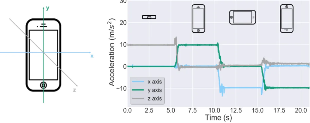
In order to understand the signal from the accelerometer sensor and its coordinate system, in Figure 2.1, it is shown in 2.1a the standard Android coordinate system and in
2.1b, the associated axis signal output with the device placed in different positions.
(a) Standard Android coordi-nate system.
(b) Sensor’s signal response to the smartphone movement.
Figure 2.1: Smartphone’s sensors standard coordinate system in Figure 2.1a, and
ac-celerometer’s output signal with the device positioned into different orientations in Figure
2.1b.
As expected, when the sensor is laid horizontally up on a platform, as in the first
5s, the accelerometer’s signal on the y andx axis reads a magnitude of approximately
0m/s2since the device is at rest, while thez axis signal reads approximately 9.81m/s2,
corresponding to the device having a null acceleration minus the force of gravity, which
is approximately 9.81m/s2. Likewise, with the smartphone upright, the accelerometer’s
signal on the y axis reads a magnitude of approximately 9.81m/s2 due to the force of
gravity, while thexandzsignal axis read a value close to 0. Leading to the conclusion,
that, through the comparison of the accelerometer’s signal values on the different axis, it is
2 . 1 . W E A R A B L E A N D S M A R T P H O N E S E N S O R S
2.1.2 Gyroscope
The gyroscope is a motion sensor that measures the rate of rotation, i.e. the angular velocity of the device in radians per second (rad/s) around three axis: yaw, pitch and roll, shown in Figure 2.2a [25].
Furthermore, the angular position is obtained through the integration of the device’s changes around the orientation axis over time, according to Equation 2.3 [5]:
θp(t) =
Z t
t0
˙
θp(t)dt+θp0 (2.3)
Wherep={Yaw, pitch, roll}andθp0 is the initial angle compared to the earth’s axis
coordinates inradians[5].
Regarding HAR, the gyroscope is majorly used to detect transitional postural activities, such as laying to standing and, along with the accelerometer sensor, the device’s position and orientation.
Similarly as for the accelerometer sensor, a study was performed in order to under-stand the gyroscope’s output signal and its coordinate system. Hence, in Figure 2.2, it is
shown the sensor’s signal while the device is placed in different positions. As expected,
Roll
Pitch
Yaw
(a) Standard Android coordi-nate system.
(b) Sensor’s signal response to the smartphone movement.
Figure 2.2: Smartphone’s sensors standard Gyroscope coordinate system in Figure 2.2a,
and gyroscope’s output signal with the device positioned into different orientations in
Figure 2.2b.
in contrast to the accelerometer, the gyroscope’s signal maintains stable values while
in the different positions, exchanging its output value during the positions’ transitions.
C H A P T E R 2 . T H E O R E T I CA L BAC KG R O U N D
2.1.3 Barometer
The barometer is an environmental sensor that measures the ambient air pressure. At-mospheric pressure can be defined as the force per unit area exerted by the overhead atmosphere molecules, varying exponentially roughly by 1 hPa (1mbar) for every 10m increase in altitude, according to Equation 2.4 [26].
P=P0e− mgh
kT (2.4)
Where p0is the pressure at the referential point, g the gravitational field strength,
h the height above the referential point, m the average mass of an air molecule, k the
Boltzmann constant (1.38065031023)J/K and T the temperature in K [26].
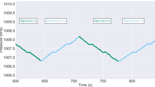
Hence, air pressure will show significant variations across a building height, allowing the discrimination of vertical movements with alterations in altitude, such as climbing up or down the stairs, as seen in Figure 2.3.
600
650
700
750
800
Time (s)
1006.0
1006.5
1007.0
1007.5
1008.0
1008.5
1009.0
1009.5
1010.0
Pre
ssu
re
(hPa
)
Upstairs Downstairs Upstairs Downstairs
Figure 2.3: Barometer’s output signal from a user climbing up and downstairs.
Indeed, as observed, as the user goes up a few flairs of stairs in the first approximately 45s, the air pressure significantly decreases. Followed by the user going downstairs, where an increase in air pressure is observed. Thus, in contrast to the prior sensors, the barometer is independent of the smartphone’s position and orientation in relation to the user’s body [27].
2 . 2 . M AC H I N E L E A R N I N G
2.2 Machine Learning
In 1959, during the primordial times of Machine Learning, Arthur Samuel defined Ma-chine Learning as “the field of study that gives computers the ability to learn without being explicitly programmed” [28]. In other words, Machine Learning has the ability to make predictions from patterns and, in a changing environment, the ability to learn, i.e continuously increasing its performance with experience.
2.2.1 Signal Processing
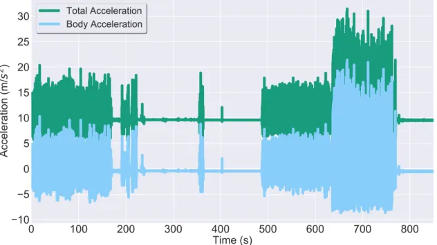
The accelerometer signal is composed by the body’s movement acceleration, the gravi-tational acceleration, intrinsic noise arising from the electronic system and movement artefacts [22]. Therefore, after the sensor’s data is extracted, the raw signal must be pro-cessed so redundancies and noise are removed. Thus, minimising the algorithm’s error, time and computational complexity. To accomplish this task, a low-pass filter is often applied to the signal. Additionally, in some cases, it may be of interest to separate the gravitational and the body acceleration component, performed by the application of a high-pass filter to the signal. Figure 2.4 displays the total body acceleration magnitude and the body movement acceleration magnitude in green and blue, respectively.
0
100
200
300
400
500
600
700
800
Time (s)
−10
−5
0
5
10
15
20
25
30
Acce
lera
tio
n (m/
s
2
)
Total Acceleration
Body Acceleration
Figure 2.4: Accelerometer signal magnitude of the total acceleration in green and the body acceleration in blue.
C H A P T E R 2 . T H E O R E T I CA L BAC KG R O U N D
Moreover, since one data sample does not correspond to one activity, in order to retrieve information from a time series, it is necessary to segment the signal into several windows. Only then, from each window, metrics are obtained and used as input to Machine Learning techniques.
There are two main types of window segmentation:staticandsliding windows. In
both, the signal is divided into equally sized windows [23], however, in the first, windows are consecutive with no gaps in between, while in the latter, a percentage of samples
are overlapped between consecutive windows so one sample can belong to two different
windows. Thus, sliding windows can be important to prevent the cut of the signal in inconvenient samples, such as during ongoing continuous cycles or transitional activities [25].
For last, in the segmentation process specifications must be predefined, such as the number of samples per windows, and, in the case of a sliding window, its overlapping
samples percentage. Furthermore, the values of those parameters require a trade-off
between the studied activity, the classifier’s final performance, its resolution, and its computational complexity. Since for simple activities a smaller window will increase the algorithm’s temporal resolution, the size of its training set and its performance, at the cost of higher computational complexity due to the higher number of windows [5]. However, for complex activities, each window may lack informative samples. Thus, requiring larger windows, where the total number of windows decreases and consequently, so does the algorithm’s computational time [5, 25, 29].
2.2.2 Feature Engineering
As stated above, from each window, the signal is not evaluated sample by sample but rather by the properties extracted from the signal in each window. These properties can be
classified according to their domain astime,frequencyandstatistical domain features
and enable the characterisation of the signal in a compact way [23, 25], enhancing its characteristics. Therefore, the chosen set of features can strongly influence the outcome of a Machine Learning algorithm.
To characterise the signal, high dimensional data is translated into a feature vector, whose size equals the number of windows and contains all the information needed to
infer each window corresponding activity. However, different features derived from
different activities may have a very different range of values. Thus, causing smaller
values to be ignored by a Machine Learning classifier while higher values are given more importance to. This tends to happen especially when the classifier involves distance measures. Therefore, it is important to normalise the feature vector values so that each feature contributes proportionately to the classifier. With this intention, in this work, each feature was scaled between 0 and 1 according to Equation 2.5 [30]:
Xscalled =
X−Xmin
2 . 2 . M AC H I N E L E A R N I N G
WhereX is the feature’s value, andXmin andXmax represent the minimum and
maxi-mum values of the feature vector values range, respectively.
In addition, to optimise the algorithm’s computational and time complexity, highly correlated features with redundant information can be removed without any loss of in-formation. Only then, through feature selection methods, the best set of features are selected, reducing the feature vector to a lower dimension and once again, the algorithm’s computational and time complexity.
Table 2.1, summarises the set of features considered in this work.
2.2.3 Classification
There are essentially three major types of Machine Learning algorithms: SL, UL and SSAL:
• InSupervised Learning (SL)is given a training set ofLsamples mapped to their
respective labels, {(xi,yi)},i= {1,...,L},xi∈Rm. Wherexidenotes the input feature
vector of dimensionm, andyiits class. Moreover, the goal is to create a hypothesis
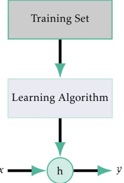
functionh:X –>Y, so thath, given a new unlabelled sample (x) is able to predict its class (y), as depicted in Figure 2.5 [31, 32].
Wheny takes the form of discrete values, this process is entitled a classification
problem, as in the case of HAR, where, for each sample corresponding to an activity,
for example walking, it will be attributed a class label valuey.
h
Learning Algorithm Training Set
x y
Figure 2.5: Pipeline description ofSupervised Learning, where a functionhgiven a new
unlabelled sample (x) is able to predict its class (y) [31].
Moreover, the process of mapping each sample to their labels in the ground truth
C H A P T E R 2 . T H E O R E T I CA L BAC KG R O U N D
Table 2.1: Statistical, Temporal and Spectral Domain Features extracted from the sensors’ signals to use in the present work.
Statistical Skewnessmeasures the asymmetry of the signal distribution
Kurtosismeasures the distribution shape around a normal distribution
Histogramplots the number of members for each bin against a total given number
of bins
Meanmeasures the signal arithmetic mean
Variancemeasures the dispersion of the signal value
Standard Deviationmeasures the dispersion of the signal values
Interquartile Rangecomputes the difference between the upper and lower quartile
Temporal Maxcomputes the signal maximum value
Mincomputes the signal minimum value
Centroidcomputes the arithmetic mean position of all the signal points
Root Mean Squarecomputes the square root of the arithmetic mean of the square
of the signal values
Median Absolute Deviation computes the median distance between each data
value and the signal median value
Zero Crossing Ratecomputes the rate at which the signal sign changes
Autocorrelationcomputes the correlation of a signal with a lagged version of itself
Linear Regressioncomputes the linear regression of the signal
Spectral Max Frequencycomputes where the FFT reaches its 95% of distribution
Median Frequencycomputes where the FFT reaches its 50% of distribution
Fundamental Frequency computes the frequency corresponding to the greatest
common divisor of all the frequency components in the signal
Max Power Spectrumcomputes the maximum value of the power spectrum density
along a given axis.
Total Energycomputes the total energy of the signal given by the squared sum of
the spectral coefficients normalised by the length of the sample windows
Spectral Centroidcomputes the weighted mean position of the signal frequencies
distribution and their probability
Spectral Spreadmeasures the variance of the signal frequencies asymmetry
distri-bution
Spectral Skewnessmeasures the asymmetry of the signal frequencies distribution
Spectral Kurtosismeasures the signal frequencies distribution shape around a
nor-mal distribution
Spectral Slope measures how quickly the spectrum decreases towards the high
frequencies
Spectral Decreasemeasures the decrease on the spectral amplitude though its
lin-ear regression computation
Spectral Roll Oncomputes the frequency so that 5% of the signal energy is
con-tained below of this value
Spectral Roll Offcomputes the frequency so that 95% of the signal energy is
con-tained below of this value
Curve Distancecomputes the euclidean distance of the signal’s cumulative sum of
the FFT elements to the linear regression
Spectral Variationcomputes the spectral variance from the cross-correlation of two
2 . 2 . M AC H I N E L E A R N I N G
must be performed manually by the user, being a difficult, time-consuming,
error-prone activity and sometimes impossible, as the ground truth information may be impossible to infer.
Additionally, the collection of a large amount of labelled data, necessary to increase the algorithm’s performance and its ability to generalise correctly into new, and previously unseen data, involves a high volume of data that consequently increases the algorithm’s computational and time complexity.
On this account, this dissertation focuses on the development of a framework with reduced manual annotation cost for the user and labelled data scalability. More-over, we introduce next some of the most common SL techniques applied in HAR, replicated in this thesis in order to incorporate the best performing model into the proposed framework and compare its results:
– k-NN classifies each sample according to the most frequent class among its
nearestk,k∈N, neighbours. Moreover, generally speaking, larger values fork
result in a more robust classifier, less susceptible to noise. However, at the cost of a less fitted decision boundary to the training samples [5, 29]. Furthermore, the overall performance of the classifier is highly influenced by the applied distance metric, which must be defined to better fit the dataset [33]. In the table 2.2 it is exhibited some of the most commonly used distance metrics and their respective math formula.
Table 2.2: Commonly used distance metrics to obtain the distance between two samples
(xandy) and their respective math formula.
Distance Metric Formula
Euclidean D(x,y) =pPmi=1(xi−yi)2
Manhattan D(x,y) =Pm
i=1|xi−yi| Chebyshev D(x,y) = maxmi=1|xi−yi| Minkowskiorder r D(x,y) = (Pmi=1|xi−yi|r)1/r
– Decision Treecreates a three like sets of if-then-else rules at each node, from
which a sample is carried on following the branches yielding the more infor-mation until it reaches a terminal node indicating its predicted output [5, 29, 33]. Moreover, the maximum depth of the tree must be defined in order to avoid overfitting to the training set [29].
– Random Forest generates multiple Decision Trees from different subsets of
C H A P T E R 2 . T H E O R E T I CA L BAC KG R O U N D
to the split into different branches. Each tree outputs a different prediction,
contributing as a vote for the final averaged output [33].
– SVMfinds the hyperplane that maximises the distance between two different
classes in the feature space. The samples having the closest distance to the hyperplane, define the classes decision boundary and are named support vec-tors. In this sense, SVM is a binary classifier, that in order to be extended to a multi-class problem, a set of multiple binary classifiers must be created, consequently augmenting the time and complexity cost of the algorithm [5, 33].
– AdaBoostcreates an ensemble of classifiers to test on weighted randomly
se-lected samples from its training set. Moreover, each consecutive classifier is fitted with the adjusted weights enhancing the incorrectly predicted samples so each consecutive learner is trained in error-prone instances [30].
– Gaussian Naive Bayes is based on the application of the Bayes theorem to
create the decision boundary function [33]:
P(y|x1, x2, ..., xm) =
P(y)P(x1, x2, ..., xm|y)
P(x1, x2, ..., xm)
(2.6)
Whereyis the predicted output class and (x1,x2,...,xm) a dependent sample
feature vector withmfeatures.
Moreover, under the assumption that every pair of features are independent,
the Gaussian Naive Bayes classifier assigns each samplexito a classyaccording
to the following equation [30]:
ˆ
y= arg max
y
P(y)
m
Y
i=1
P(xi|y) (2.7)
Wherep(y) is estimated usingMaximum A Posterioriestimation and the
likeli-hood of the features is assumed to be Gaussian so:
P(xi|y) =q 1 2πσy2
exp
−
(xi−µy)2
2σy2
(2.8)
Whereσyandµy are estimated using maximum likelihood.
– Quadratic Discriminant Analysis (QDA)fits a Gaussian density to each class
generated by by fitting class conditional densities to the data and using Bayes’ rule to return a quadratic decision boundary. Assumes the covariance matrix
to be different for each class, hence, it will estimate the covariance matrix
2 . 2 . M AC H I N E L E A R N I N G
• Unsupervised Learning (UL)includes Clustering, Dimensionality Reduction, Anomaly
Detection and Quantile Estimation. This work will focus on the former.
In a clustering problem, we are given a training set ofU samplesXU = {x1,x2, ...,
xU},i= {1,...,U}. Wherexi ∈Rmdenotes the input feature vector of dimension m,
however, in contrast to SL, in UL it is not given any labelsyi [32].
In essence, a clustering algorithm finds structure on the feature space where no prior
information is given and divides it into different clusters. Moreover, an effective
clustering algorithm should maximise intra-cluster similarities and minimise inter-cluster similarities so homogeneous and well-separated groups are created [22].
Likewise as for SL, we introduce next some of the most common clustering tech-niques applied in HAR, replicated in this thesis in order to compare its results to the obtained by the algorithms developed in this dissertation:
– InK-Meansthe unlabelled dataset is divided intokclusters. Initially,kpoints
are chosen randomly as cluster centres, named centroids. Then, each sample is assigned to the closest centroid cluster, re-calculating the cluster’s centroid as the centre of all samples in each cluster. This process is repeated as the
samples are assigned to a different cluster and the centroids adjusted. Some of
this algorithm’s main characteristics are its low time complexity, the fact that it changes significantly with the initial cluster partition, the creation of spherical and equally sized clusters, and the requirement of the number of clusters as an input parameter [22].
– Mini Batch K-Meansis very similar toK-Means, distinguishing fromK-Means
by the use of subsets of the dataset with a fixed size, mini-batches, instead of using the entire dataset. Thus, minimising the algorithm’s time and computa-tional complexity, however, at the cost of a loss in the classifier’s performance [22].
– Spectral ClusteringappliesK-Meansclustering to the projection of normalised
eigenvectors obtained from the Laplacian of the samples’ similarity graph. This method is especially useful to create clusters with non-convex bound-aries.
– InDensity-Based Spatial Clustering of Applications with Noise (DBSCAN)
C H A P T E R 2 . T H E O R E T I CA L BAC KG R O U N D
– Gaussian Mixtureconsists of a probabilistic model generating clusters from
a mixture of Gaussians distributions with unknown mean and covariance, fit-ted to the feature space data through the implementation of the expectation-maximisation algorithm. Moreover, this method allows to easily describe un-usual distributions and, along with DBSCAN, does not require the number of clusters as an input parameter.
In the final analysis, UL techniques’ biggest advantage is having no annotation cost, as they do not require the input samples to be labelled. However, this fact comes at the cost of not knowing the samples’ ground truth labels, necessary to ascertain the classifier’s results. Thus, since HAR models should return a label indicating the performed activity, the HAR systems tend to be supervised or semi-supervised [6].
Therefore, this thesis focuses on a hybrid setting between SL and UL,Semi-Supervised
Learning, with the goal of enhancing the positive aspects of both. That is, to obtain the SL good results and obtain the respective samples’ class labels, with UL small scalability and annotation cost.
• InSemi-Supervised Learning (SSL)in addition to the labelled data, the classifier
incorporates additional information incorporated in new unlabelled samples (easily available at a large scale) to enhance the its performance and reach a more accurate prediction. Thus, the datasetXis partitioned into the labelled samplesXL= {x1,x2,
..., xL} mapped to the labelsYL = {y1, y2, ...,yL} and the unlabelled samplesXU =
{xL+1,xL+2,...,xL+U} for which the labels are unknown [32].
Hence,Semi-Supervised Learningallows to achieve similar results as implementing
SL, but with smaller annotation cost, as there is a significantly less amount of la-belled data. With this in mind, since the goal of this dissertation is to decrease the
annotation cost of the SL techniques, Semi-Supervised Learning was the Machine
Learning type of learning methodology chosen to be implemented in this disserta-tion.
Moreover, this work will implement three types ofSemi-Supervised Learning: ST, AL
and PL.
– InActive Learning (AL)a selective sampling function selects from the large
unlabelled dataset (also referred as pool set) the samples which are more infor-mative to be labelled and added to the classifier’s labelled training set. Further-more, the samples considered more informative, are usually the samples with the highest gain for the classification process, so that, with a lower amount of
labelled data and therefore, lower data volume and manual annotation effort
from the user, it is possible to reach a classification performance similar to SL.
Thus, as presented in Figure 2.6, firstly, in order to learn the model’s
2 . 2 . M AC H I N E L E A R N I N G
Model Input Data
Labelled Data (L)
Oracle Annotation
Unlabelled Data (U)
Figure 2.6: Pool-based AL cycle. Where in every iteration the oracle annotates a new sample that is integrated into the model’s training set. Followed by an update of the model with its new, augmented training set.
large unlabelled dataset (U), through a QS (Q), it is selected for the oracle
to annotate, the most informative sample (x∗). This process is then repeated
iteratively until a Stopping Criterion (SC) is met. Hence, initiallyL << U,
how-ever in how-every iteration, the newly annotated samplex∗is removed fromU and
added toL. Incrementing the labelled train set and consequently, reducingU
[14, 34].
Figure 2.7 shows through a two-dimensional Principal Component Analysis (PCA), the growth of the labelled training set throughout the iterations as the oracle annotates one sample per iteration. Moreover, one dot represents one sample whose colour indicates the class that it belongs to so that samples with the same colour belong to the same class.
Figure 2.8 shows the classifier’s prediction on the test set samples through a two-dimensional PCA, where each dot embodies a test data sample whose colour represents its predicted class.
C H A P T E R 2 . T H E O R E T I CA L BAC KG R O U N D
−0.25
0.00
0.25
0.50
−0.5
0.0
0.5
Co
mp
on
en
t 2
Iteration 0
−0.5
0.0
0.5
−0.5
0.0
0.5
Iteration 150
−0.5
0.0
0.5
Component 1
−0.5
0.0
0.5
Co
mp
on
en
t 2
Iteration 300
−0.5
0.0
0.5
Component 1
−0.5
0.0
0.5
Unlabelled Samples
Figure 2.7: Growth of the AL training set from iteration 0 till iteration 300 and the remaining unlabelled samples on the pool set, on a two-dimensional PCA. Each dot embodies a data sample whose colour represents its class. Example performed using the University of California, Irvine (UCI) dataset [35].
−0.5
0.0
0.5
−0.5
0.0
0.5
1.0
Co
mp
on
en
t 2
Iteration 0
−0.5
0.0
0.5
−0.5
0.0
0.5
1.0
Iteration 150
−0.5
0.0
0.5
Component 1
−0.5
0.0
0.5
1.0
Co
mp
on
en
t 2
Iteration 300
−0.5
0.0
0.5
Component 1
−0.5
0.0
0.5
1.0
Ground Truth
2 . 2 . M AC H I N E L E A R N I N G
– Passive Learning (PL)follows the same methodology as AL, but there is no
selective sampling function. Instead, the sample is randomly selected from the unlabelled dataset.
– InSelf-Training (ST)a classifier is trained on the available labelled dataset
and posteriorly tested on the unlabelled dataset. Then, test samples having the higher prediction confidence score are added to the classifier’s training set and removed from the unlabelled dataset. This process is repeated iteratively as the classifier is re-trained on an increasingly larger and larger training set, increasing its performance.
Therefore, under the assumption that highly confident predicted labels are correct, the learner uses its own predictions to iteratively teach himself, con-sequently improving its performance till the unlabelled data set is exhausted, and all the samples become labelled [36], as shown in Figures 2.9 and 2.10. Moreover, comparing both figures similarly as performed for the AL process, the learner starts at iteration 0 with a very poor prediction due to its small non-representative training set, verified by the fact that all samples are predicted as belonging to the same class (since they present the same colour). Nevertheless, as the classifier’s training set grows (from iteration 0 to iteration 300), through the addition of highly confident predicted samples to the learner’s training set, its performance increases until its predictions match the ground truth data, as observed in the plot in the lower right corner in Figure 2.10.
Additionally, due to the ST ability to grow and teach himself with the available unlabelled data, the learner’s training set size in the iterations 150 and 300 in Figure 2.10 present a significant growth of the train set data volume in comparison to the obtained in the AL process shown in Figure 2.8, iterations 150 and 300. This fact was expected since the later only increments its training set 1 sample per iteration (the sample that the user annotated) while ST adds to its training set all the samples that it is able to predict with high confidence.
To conclude, as has been noted, both Semi-Supervised Learning, ST and AL
address the issue that labelled data is scarce and difficult to obtain. Therefore,
they focus on the information that can be derived from the unlabelled data while preserving a reduced annotation cost and volume data scalability.
Moreover, while AL explores the unknown (choosing unlabelled data to be
annotated),Semi-Supervised Learning, uses what has known to exploit the
C H A P T E R 2 . T H E O R E T I CA L BAC KG R O U N D
−0.25
0.00
0.25
0.50
−0.5
0.0
0.5
Co
mp
on
en
t 2
Iteration 0
−0.5
0.0
0.5
−0.5
0.0
0.5
Iteration 150
−0.5
0.0
0.5
Component 1
−0.5
0.0
0.5
Co
mp
on
en
t 2
Iteration 300
−0.5
0.0
0.5
Component 1
−0.5
0.0
0.5
Unlabelled Samples
Figure 2.9: Growth of the ST training set from iteration 0 till iteration 300 and the remaining unlabelled samples on the pool set, on a two-dimensional space PCA. Each dot embodies a data sample whose colour represents its class. Example performed using the UCI dataset.