Contextual Information based on Pervasive Sound Analysis

(1)

Ricardo Miguel Pontes Leonardo

Bachelor of Science in Biomedical Engineering

Contextual Information based on

Pervasive Sound Analysis

Dissertation submitted in partial fulfillment of the requirements for the degree of

Master of Science in Biomedical Engineering

Adviser: Hugo Filipe Silveira Gamboa, Professor Auxiliar, Faculdade de Ciências e Tecnologias, Universidade Nova de Lisboa

Examination Committee

Chairperson: Prof. Dr. Carla Maria Quintão Pereira

Raporteur: Prof. Dr. Ricardo Nuno Pereira Verga e Afonso Vigário Member: Prof. Dr. Hugo Filipe Silveira Gamboa

(2)

(3)

Contextual Information based on Pervasive Sound Analysis

The Faculty of Sciences and Technology and the NOVA University Lisbon have the right, perpetual and without geographical boundaries, to file and publish this dissertation through printed copies reproduced on paper or on digital form, or by any other means known or that may be invented, and to disseminate through scientific repositories and admit its copying and distribution for non-commercial, educational or research purposes, as long as credit is given to the author and editor.

This document was created using the (pdf)LA_{TEX processor, based in the “novathesis” template[1], developed at the Dep. Informática of FCT-NOVA [2].}

(4)

(5)

"Se perderes a direção da lua, Olha a sombra que tens colada aos pés"

(6)

(7)

A c k n o w l e d g e m e n t s

First and foremost, I would like to express my deepest gratitude to my supervisor, Profes-sor Hugo Gamboa, for welcoming me atFraunhofer AICOSand being an excellent advisor throughout the whole project. Thank you for the great guidance and the dedication, as well as for making me grow as a professional. Thank you also for reinforcing my love for data science, both before as a professor and now as a supervisor.

I would also like to thankAssociação Fraunhofer Portugal Researchfor all the support and the opportunity of working on my thesis in a company environment. A word of appreciation in particular to everyone in the Lisbon, team for being the living proof that a work environment can and must be fun in order to be productive. A very special thanks to Marilia Barandas for all the patience for me and the constant support, your help was invaluable. Also a word of gratitude for my colleague David Melo for his great friendship and for accompanying me throughout this experience.

Thanks to all my college friends, I could fill a book with my gratitude for all of you. Thank you for all the laughs, and for all those silly moments that make life worth living. I couldn’t have done this without you.

And last but not least, I thank my family for always being there for me, both in moments of joy and hardship. The most heartfelt thanks to my parents, to whom I owe everything I am and who always believed in me. Words are not enough to describe how thankful I am. I love you all.

(8)

(9)

A b s t r a c t

In recent times, there has been a continuous increase in the ubiquity, processing power and sensing capabilities of modern smartphones. This has made possible the emergence of new technologies that allows users to keep track of information regarding their health, activities and location, even in indoor places were GPS signal is not available. These technologies typically rely on fusing and processing information coming from multiple sensors, such as the accelerometer or the magnetometer.

This thesis proposes a framework for indoor location and activity recognition from new source of information: the sound perceived through the device’s microphone. It does so by extracting information relative to the user’s position and activities through machine learning and audio processing techniques.

In the context of indoor location, the proposed SoundSignature algorithm allows the device to learn from labeled data and predict the location it is in. These locations may be different rooms or distinct regions of large places, such as open spaces.

Another proposed algorithm, SoundSimilarity, further refines this positioning by com-paring the sound signals from two or more devices in real time. A novel audio similarity metric identifies if the devices are close to one another, mitigating the potential errors of the SoundSignature algorithm. This also has many other use cases, such as detecting proximity between the user and devices.

Finally, the Activity Monitoring algorithm allows the device to learn from labeled data to recognize the activity the user is performing. This information may be also used to further refine the location algorithm by recognizing location-dependent activities such as the closing of doors or watching television.

Keywords: Indoor Location, Human Activity Recognition, Machine Learning, Signal Processing, Audio Analysis

(10)

(11)

R e s u m o

Nos últimos tempos, tem havido um aumento contínuo da ubiquidade, poder de pro-cessamento e capacidade sensorial nossmartphonesmodernos. Isto possibilitou o apareci-mento de novas tecnologias que permitem aos utilizadores monitorizar informações sobre a sua saúde, atividades e localização, mesmo em zonas interiores onde o sinal GPS não está disponível. Estas tecnologias geralmente dependem de processamento de informação proveniente de vários sensores tais como o acelerómetro ou o magnetómetro.

A presente tese propõe umaframeworkpara localização em zonas interiores e reconhe-cimento de atividade através de uma nova fonte de informação: o som percebido através do microfone do dispositivo. Para tal, o sinal é processado com técnicas demachine lear-ninge de processamento de sinal.

No contexto da localização em espaços interiores, o algoritmoSoundSignaturepermite que o dispositivo aprenda com dados rotulados e identifique a localização em que se encontra. Esses locais podem ser divisões diferentes ou regiões distintas de locais amplos.

Outro algoritmo,SoundSimilarity, compara os sinais de som de dois ou mais disposi-tivos em tempo real com uma métrica de similaridade de áudio para identificar se estes estão próximos uns dos outros. Isto não só ajuda a mitigar potenciais erros do algoritmo anterior como também pode ser aplicado noutros casos, tal como detetar a proximidade entre o usuário e outros dispositivos.

Finalmente, o algoritmoActivity Monitoringpermite que o dispositivo aprenda com dados rotulados para identificar a atividade que o utilizador está a realizar. Esta informa-ção pode também ser utilizada para para localizar o utilizador ao reconhecer atividades dependente de Esta informação pode também ser usada para auxiliar os algoritmos de lo-calização, reconhecendo atividades dependentes da localização tais como fechar portasou ver televisão.

Palavras-chave: Localizaçãoindoor, Reconhecimento de Atividades Humanas, Aprendi-zagem Automática, Processamento de Sinal, Análise de Áudio

(12)

(13)

C o n t e n t s

List of Figures xv

List of Tables xvii

Acronyms xix

1 Introduction 1

1.1 Context and Motivation. . . 1

1.2 Objectives . . . 2

1.3 Literature Review . . . 2

1.4 Thesis Overview . . . 4

2 Theoretical Background 5 2.1 Machine Learning . . . 5

2.1.1 Preprocessing . . . 6

2.1.2 Feature Extraction. . . 6

2.1.3 Classification . . . 6

2.1.4 Feature Selection . . . 10

2.1.5 Validation . . . 11

2.2 Sound Analysis . . . 12

2.2.1 Frequency Domain . . . 14

2.2.2 Mel Frequency Scale . . . 14

2.2.3 Audio Features . . . 14

3 Proposed Framework 17 3.1 SoundSignature: Indoor Location based on Background Spectrum Analysis 17 3.1.1 Acoustic Fingerprint Extraction . . . 18

3.2 SoundSimilarity: Proximity Detection from Real-time Comparison of Au-dio Signals . . . 20

3.2.1 Cross-Correlation . . . 21

(14)

C O N T E N T S

3.2.2 Measuring the Similarity of Audio Segments . . . 22

3.2.3 Binary Classification . . . 24

3.3 Activity Monitoring . . . 25

3.3.1 Preprocessing . . . 26

4 Results 29 4.1 SoundSignature . . . 29

4.1.1 Proof of Concept . . . 29

4.1.2 Data Acquisition . . . 30

4.1.3 Results . . . 31

4.2 SoundSimilarity . . . 33

4.2.1 Data Acquisition . . . 33

4.2.2 Data Processing . . . 34

4.2.3 Receiver Operating Characteristic (ROC) curve analysis . . . 34

4.2.4 Results . . . 35

4.3 Activity Monitoring . . . 35

4.3.1 Dataset . . . 35

4.3.2 Results . . . 36

5 Conclusion and Future Work 39 5.1 Conclusion . . . 39

5.2 Future work . . . 41

Bibliography 43

A Paths for the SoundSignature Dataset 47

(15)

L i s t o f F i g u r e s

2.1 Bidimentional illustration of Support Vector Machines. w~·~x+b= 0 indicates the found hyperplane that ideally separates the two classes;w~·~x+b= 1 and

~

w·~x+b=−1 delineate the margin between the classes. The points of different

colors indicate samples of different classes, and the outlined ones represent

the used support vectors. . . 8

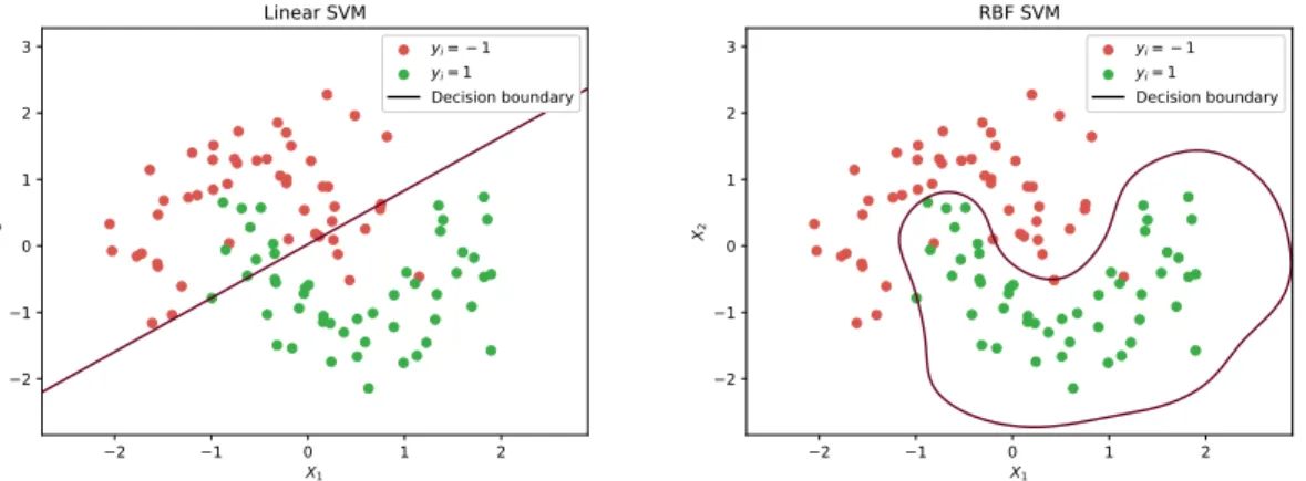
2.2 Comparison of the decision boundaries found in a bidimensional feature space with and without using the kernel trick. . . 9

2.3 Fluxogram explaining the Sequential Forward Feature Selection algorithm . 11

2.4 Comparison between a sound wave and its representation as an audio sig-nal. Below is the propagation of a sound wave where the dots represent air particles, C zones of compression and R zones of rarefaction. Above is the representation of this sound as an audio signal. (How to cite image from wikimedia commons?) . . . 13

2.5 Quantization of a continuous signal. The bit depth is 3 bits and the sampling rate is 10000 Hz. . . 13

2.6 Diagram explaining how to compute Mel Frequency Cepstral Coeffi_cients

(MFCC). . . 15

3.1 Schematic representation of the SoundSignature algorithm. . . 17

3.2 In this spectrogram of an segment of audio data we can visually discriminate two distinct components: a background noise spectrum that remains con-stant throughout the signal and transient sounds of larger intensity that are addictive to this spectrum. . . 18

3.3 Schematic representation of the SoundSimilarity algorithm. . . 21

3.4 Illustration of periodic summation. This process consists of taking a signal limited in time and repeating it from−∞to∞, creating a periodic signal. . . 22

3.5 Comparison between two cases for circular cross-correlation of audio signals recorded at the same time. . . 22

3.6 Graph of the absolute values of a correlation with a peak, normalized to [0,1].

MASf ,g will be equal to the maximum inRminus the maximum inR. . . 23

3.7 Graphic of the Measurement for Audio Similarity (MAS) over time between two signals and comparison between before and after filtering. . . 24

(16)

L i s t o f F i g u r e s

3.8 ROC curve depicting Youden’s J statistic. . . 25

3.9 Schematic representation of the activity monitoring algorithm. . . 26

4.1 Normalized confusion matrix of the dataset used for proof of concept. . . 30

4.2 Normalized confusion matrix of the SoundSignature algorithm with the SoundSig-nature for classification within the locations.. . . 32

4.3 Normalized confusion matrix of the SoundSignature algorithm with the SoundSig-nature for diff_{erentiating locations.} _{. . . .} ₃₃

4.4 Result of the classification of the test route. Below is the ground truth; above is the result of the classification. . . 33

4.5 Illustration of a path designed for data acquisition for the SoundSimilarity algorithm. The red microphone symbol represents the stationary microphone, the blue circle represents the starting position and the green line represents the path the user takes while holding a sound recording device.. . . 34

4.6 ROC curve for the MAS. . . 35

4.7 Result of the SoundSimilarity algorithm, compared to the ground truth. In the represented example an airplane redying for landing passed over the building while the two devices were in different locations, meaning that both recorded

its characteristic sound. This means that both recorded the same sound, pos-sibly generating wrong results. However, the MAS not only showed itself resilient to this event but also the threshold adapted to this scenario. . . 36

4.8 Normalized confusion matrix for the Activity Recognition algorithm. . . 37

A.1 Plant of the ground floor of the building where the acquisitions for the SoundSig-nature dataset where made. In this plant we can see the designed routes and their respective labels. . . 48

A.2 Plant of the first floor of the building where the acquisitions for the SoundSig-nature dataset where made. In this plant we can see the designed routes and their respective labels. . . 49

(17)

L i s t o f Ta b l e s

4.1 Composition of the dataset used for proof of concept. . . 29

4.2 Composition of the SoundSignature dataset. . . 31

4.3 Composition of the dataset used activity recognition. . . 37

(18)

(19)

A c r o n y m s

AUC Area Under the Curve.

DTW Dynamic Time Wrapping.

GNSS Global Navigation Satellite System.

GPS Global Positioning System.

HAR Human Activity Recognition.

MAS Measurement for Audio Similarity.

MFCC Mel Frequency Cepstral Coefficients.

OvO One-vs-one.

OvR One-vs-rest.

rbf radial basis function.

ROC Receiver Operating Characteristic.

SVM Support Vector Machines.

(20)

(21)

C

h

a

p

t

e

r

1

I n t r o d u c t i o n

1.1 Context and Motivation

In recent times, there have been major developments in the smartphone industry. Their ever increasing processing power and continuous connection to the Internet have made them essential part of our lives, both as work and entertainment tools. This, allied to their also ever increasing sensing capabilities, increased the market’s interest inHuman Activity Recognition (HAR)technologies.

HAR is a field of computer science that integrates sensor data with machine learn-ing algorithms to recognize a wide range of human activities such as brushlearn-ing teeth or walking [4]. This creates new technologies that allow users to better keep track their daily habits and improve their lifestyle. Other use cases include assisting caretakers in the monitoring of elderly people or reminding rehabilitation patients to execute their prescribed exercises.

These technologies typically rely on tracking the device’s movements through sensors such as the accelerometer or the magnetometer. However, the use of these sensors require that the device is attached to the user, commonly in specific body locations. Furthermore, relying on movement exclude the detection of certain activities that do not incur in it, such as talking or watching television.

Other field where smartphones are used everyday is in navigation systems and location-dependent services. In this context, the most well known and widespread technology is

Global Positioning System (GPS), included in the Global Navigation Satellite System (GNSS). However, while this system’s precision and satellite coverage are typically suffi

-cient for outdoor applications, this is not the case when the user is inside a building. The presence of walls and ceilings between the user and the satellites greatly attenuates the latter’s signal, and the reduced scale of typical paths in buildings compared to outdoor

(22)

C H A P T E R 1 . I N T R O D U C T I O N

routes create a demand for better precisions.

These deficits in both HAR and indoor location created a need for new sources of information for these activities. As such, in the present work we study the analysis of pervasive sound as a source of contextual information in these two contexts.

1.2 Objectives

As the responsible for one of the five traditional senses, our auditory system is constantly picking up large amounts of information about our surroundings. This information may be event-dependent, such as walking or the closing of doors, or location-dependent, such as the humming of computers or air conditioning systems. The aim of this thesis is to translate this innate ability of ours to any microphone equipped mobile device.

This thesis presents an original framework developed for extracting information from sound regarding the user’s position and the activities they are performing. For this purpose, three algorithms were created:

1. SoundSignature: Recognizes the location the user is in. These locations consist of different rooms or distinct regions of large spaces. Relies on machine learning

techniques to learn from labeled data.

2. SoundSimilarity:Extracts a novel measurement of audio similarity from the sounds perceived in real time by two or more devices, allowing it to identify if these are in the same location.

3. Activity Monitoring:Analyses pervasive sound to recognize activities the user per-forms. Similarly to the SoundSignature algorithm, relies on machine learning tech-niques to learn from labeled data.

1.3 Literature Review

Multiple alternative solutions have been proposed in the literature for indoor positioning systems. Many leverage signals transmitted between beacons and the device to be located, namely Radio Frequency signals, either Wi-Fi [15] or Bluetooth [6], infrared signals [10], ultrasound [2], visible light [21], among others. By estimating the distance of the device to each beacon through metrics such as received signal strength (RSS) [31] and time difference of arrival (TDoA) [18], trilateration may be used to locate the device. Other

methods include using these metrics for fingerprinting techniques [3]. However, most of current systems rely on infrastructure, leading to elevated setup and maintenance costs. Some infrastructure-free solutions have also been proposed, such as using pervasive signals such as ambient light [16] and perturbations in the Earth’s magnetic field for fingerprinting techniques [17]. Novel systems integrate many of the afore mentioned developments with inertial tracking and map data to locate the user indoors [9]. An

(23)

1 . 3 . L I T E R AT U R E R E V I E W

existing sound-based solution by Stephen P. Tarzia et al. [27] uses the power spectra the audio signal as an acoustic fingerprint to differentiate between different rooms [27].

Furthermore, Jun-Wei Qiu and Yu-Chee Tseng [22] have shown that meetings between two or more users may be used to calibrate their respective potential locations. Sound-based proximity detection was achieved through use of the normalized cross-correlation coefficient between the spectra of the compared signals [23].

Regarding the context ofHAR, multiple solution have been developed about identi-fying the user’s activities from recorded sound. The most transversal element to them is the use ofMFCC, a group of features based on the human perception of pitch. These features are commonly used in speaker [28] and speech recognition [12].

Yi Zhan et al. [34] employ these features forHAR. The authors split a sound segment into windows of smaller length and for each of theseMFCCwere extracted. The resulting matrix is then compared to previously recorded and labeled templates through the use of aDynamic Time Wrapping (DTW)algorithm, achieving an accuracy of 92.5%.

Johannes A. Stork et al. [26] also employMFCCas features, but instead use a Random Forests algorithm for classification. This method achieved an accuracy of 85.8%.

Yao Yang et al. [32] use features such as Spectral Centroid and Spectral Roll-offto

pre-liminarily determine if the recorded sound consists of speech, music or a human activity such as brushing teeth. After this stepMFCCare once again employed to determine the activity.

Yi Zhan and Tadahiro Kuroda [35] released another study regardingHAR, this time employing features extracted from a continuous wavelet transform with Haar wavelets. To these they called "Haar-like features". The chosen classifier was Hidden Markov Mod-els and the achieved accuracy was 96.9%. For comparison, the authors used the same algorithm and dataset but recurring toMFCCinstead of these "Haar-like features"and the accuracy dropped to 88.7%.

Jia-Ching Wan et al [30] elaborate on previous work by applying Individual Compo-nent Analysis to the MFCC, generating artificial features with high statistical indepen-dence between them. For classification, aSupport Vector Machines (SVM)classifier was used, achieving an 86.7% accuracy.

Etto L. Salomon et al. made a thorough comparison of features and classifier algo-rithms in the context of sound-basedHAR. Notably, the authors followed the protocol described in [34] and got poor results. As such, the "Haar-like features"were preliminar-ily discarded. The study concluded that the best results were obtained withMFCC as features andSVMas classifier.

Daniel Kelly and Brian Caulfield [13] used an algorithm based onMFCCandSVMfor distinguishing the sound of cutlery from the sound of tap water, achieving an accuracy of 96.9%. Applying the same algorithm to discriminating between speech, music and environmental sounds yelded an accuracy of 88.7%.

Finally, C. E. Galván-Tejada employedMFCCalong with statistical features such as standard deviation and median to distinguish between quotidian sounds. Two classifier

(24)

C H A P T E R 1 . I N T R O D U C T I O N

algorithms were compared: Random Forests, which yielded an accuracy of 81.4%, and Neural Networks, with an accuracy of 77.7%.

In conclusion, current infrastructure-free indoor location algorithms rely on finger-printing techniques or inertial sensors, the latter being irrelevant in the current work. Furthermore, the features most prevalent in current literature regarding sound classifica-tion areMFCCand features extracted from the frequency spectrum. Likewise the most commonly used classifier algorithm isSVM.

1.4 Thesis Overview

The present chapter introduced the motivation behind the development of the current work, as well as the main objectives and a review of the literature regarding the subject at hand. Chapter2provides some theoretical concepts about audio processing and machine learning, both relevant to this work.

Chapter3presents the developed framework, describing the methodologies used and explaining the deliberations made in their design.

Chapter4 show the results obtained, along with the composition and acquisition methods of the used datasets. Chapter5present the main conclusions of this thesis and guidelines for future work.

Finally, appendixAshows the routes used for recording the SoundSignature dataset, which will be relevant in section4.1.2.

(25)

C

h

a

p

t

e

r

2

T h e o r e t i c a l Ba c k g r o u n d

2.1 Machine Learning

In computer science, machine learning can be defined as the branch that gives computers the ability to learn without being explicitly programmed [33]. It does so by extracting features from a training set of data, allowing the algorithm to learn the underlying model and thus classify future inputs.

According to the data available to be used, there are various categories of machine learning algorithms:

• Supervised learning: The algorithm is presented with a set inputs and their respec-tive desired outputs, or labels. The goal is to generate a model that maps the inputs to the outputs.

• Unsupervised learning: The algorithm is presented with unlabeled inputs. The goal is to separate the inputs into clusters based on their similarity.

• Semi-supervised learning: The algorithm uses both a small amount of labeled data and a large amount of unlabeled data.

• Reinforced learning: Instead of learning from discrete samples of data, the algo-rithm interacts with a dynamic environment in which it must perform a certain goal, such as winning at a game of checkers or driving a car.

The problems at hand will rely on labeled data, and as such we will be focusing on supervised learning.

(26)

C H A P T E R 2 . T H E O R E T I CA L BAC KG R O U N D

2.1.1 Preprocessing

In order to apply machine learning algorithms to continuous streams of data, we must first segment it into individual inputs. This is typically done by dividing the signal into windows of equal length, which may or may not have some overlap between them.

The length of the window will have an impact on the performance of the algorithm. On the one hand, smaller windows will increase the temporal resolution and reduce com-putational costs. On the other hand, larger window lengths will provide larger amounts of data per sample, allowing better recognition.

Furthermore, increasing the size of the overlap will provide the algorithm a larger training set, at the cost of some redundancy between samples.

2.1.2 Feature Extraction

Features can be defined as properties extracted from certain input. These will be used as the input for a classifier algorithm, whether it is for training, testing or usage. They can be either continuous (such as temperature) or discrete (such as rainy or sunny), and can be classified according to the domain they operate in, such as time, statistical or frequency. Different features may have different means standard deviations, which may lead to

giving more importance to some features than others when training a classifier algorithm. Because of this, it is important to standardize all features so that they have meanµ= 0 and standard deviationσ= 1. This is achieved through the following expression:

xnorm=

x−µ

σ (2.1)

Wherex is a feature, µits mean, σ its standard deviation andxnorm the resulting stan-dardized feature.

2.1.3 Classification

A classifier is an algorithm that maps input data to a category. It does so by generating a model from a training set containing observations whose category is known. It is on the basis of these that supervised learning are built upon.

There are multiple classifier algorithms. The choice of the algorithm will depend on various parameters such as the kind of data, number of observations and number of individual categories.

Some examples of common classification algorithms are:

• TheK-Nearest Neighbors algorithm finds the closest K nearest instances in the training set and classifies it according to the most frequent class among these. K is an integer, usually small in relation to the size of the training set. Larger values for K make the algorithm more robust to noise [5], but make the decision boundary less defined. This algorithm is computationally fast in the training phase but slow in classifying inputs.

(27)

2 . 1 . M AC H I N E L E A R N I N G

• TheNaive Bayesclassifier assumes all features are independent of each other, and under this assumption calculates the probability of an input being each class given its features. This is done through the Bayes’ theorem:

P(Ck|x) =P(Ck)P(x|Ck)

P(x) (2.2)

WhereCkis the k-th class andxthe feature vector.

• Decision Treescreate a model based nodes connected by branches in a tree-like fashion. Each node contains a simple rule pertaining to a single feature. An input starts at the top node and travels down the branches guided by these rules until a terminal node is reached. These terminal nodes indicate the class the input is classified with. Decision trees are generated by computing at each node which splits yield the most information. This can be done through a number of criteria.

• Support Vector Machinesfind the hyperplanes in the feature space that best sepa-rate the training set into their labels..

• Ensemble Methodscreate multiple independent classifiers. Their predictions are then used to achieve a final result. An example of such a classifier is Random Forests, where multiple decision trees are created from diff_{erent subsets of the}

dataset. Each classifier’s prediction counts as a vote towards the predicted class. The final result is the class with the most votes.

• Neural Networksare composed of elements called perceptrons that mimic the func-tioning of neurons.

2.1.3.1 Support Vector Machines

Being the most prevalent classifier algorithm in the reviewed literature, in the present work we chose to useSVM.

SVMare binary classifiers, meaning that they can only discern between two classes. If we consider an n-dimensional space where each dimension relates to a feature, this classifier finds the hyperplanew~·~x+b= 0 that best separates the two classes.

For a given set of linearly separable pointsx~i in the feature space that map to two classesyi= 1 oryi=−1, we can assume that the margin between them can be delineated by two parallel hyperplanes w~·~x+b= 1 andw~ ·~x+b=−1, as shown in figure2.1. We want these two hyperplanes to follow two conditions:

• The distance between them, given by b

||w||, must be maximum. This means we want

to minimize||w||

• The data points cannot fall into the margin between them. We can impose that by adding the restrictionsw~·~xi+b≥1 andw~·~xi+b≤ −1. This can be simplified into

yi(w~·~xi+b)≥0.

(28)

1 2 3 4 5 6 7

X1 0 2 4 6 8 10 X2 ⃗

w ⋅ ⃗x + b = −1

⃗

w ⋅ ⃗x + b = 0

⃗

w ⋅ ⃗x + b = 1

yi= − 1

yi= 1

Support Vector

Figure 2.1: Bidimentional illustration of Support Vector Machines.w~·~x+b= 0 indicates the found hyperplane that ideally separates the two classes;w~·~x+b= 1 andw~·~x+b=−1 delineate the margin between the classes. The points of diff_{erent colors indicate samples}

of different classes, and the outlined ones represent the used support vectors.

While minimizing||w~||under this restriction finds the ideal solution for fully linearly separable datasets, this is not always the case. To extendSVMto non linear separable data, instead of applying the last restriction we introduce a hinge loss function based it. This will also be an expression we want to minimize:

max(0,1−yi(w~·~xi+b)) (2.3)

This value of this expression will be equal to zero if the point is on the right side of the plane and outside the margin. Otherwise, it will be proportional to the distance between the point and the margin.

Given these two expressions we want to minimize, the resulting hyperplane parame-ters can be obtained by minimizing the following expression:

1 n      

n−1

X

i=0

max(0,1−yi(w~·~xi+b))

    

+λ||w||

2 _(2.4)

Whereλrepresents the trade-offbetween increasing the size of the margin and

ensur-ing that the~xi lie on the correct side of the margin. This expression is only affected by

(29)

points either inside or bordering the margin. To these we call support vectors.

By minimizing this expression we obtain values forw~ andb, obtaining the hyperplane

~

w+b= 0 that functions as a decision boundary. Inputs will be classified according to in what side of this hyperplane they are on.

Additionally, a probability estimation of an input being classified can be obtained by how far it is from the decision boundary.

2.1.3.2 Kernel trick

SVMdoes its computations under the pretension that the classes are linearly separable, and as such the decision boundaries are linear. Non linear separations can be achieved by translating the feature space to higher dimensions, minimizing this expression and translating back to the original number of dimensions. This can be easily simplified by replacing every inner product ~x·~y with a kernel function k(~x, ~y). An example of such function is theradial basis function (rbf)kernel:

k(f , g) =exp(−γ(~x−~y)) (2.5)

Whereγ is a adjustable parameter greater than 0. The smaller this parameter is, the smoother will be the decision boundary. Figure2.2shows the difference between decision

boundaries found with and without the kernel trick.

−2 −1 0 1 2

X1 −2 −1 0 1 2 3 X2 Linear SVM

yi= − 1

yi= 1

Decision boundary

(a) Decision boundary found with linearSVM.

−2 −1 0 1 2

X1 −2 −1 0 1 2 3 X2 RBF SVM

yi= − 1

yi= 1

Decision boundary

(b) Decision boundary found withSVMusing the

rbfkernel.

Figure 2.2: Comparison of the decision boundaries found in a bidimensional feature space with and without using the kernel trick.

2.1.3.3 Extension to multiclass problems

To extend binary classification algorithms to multiclass problems withkclasses there are two common procedures:

(30)

• One-vs-rest (OvR)createsk classifiers, or one per class. Each classifier considers

the samples from that class as positive and the remaining as positive. The chosen class will be the one whose classifier reports the largest confidence score.

• One-vs-one (OvO)createsk(k−1)/2 classifiers, one for each possible pair of classes.

The prediction of each classifier will vote towards the overall prediction.

2.1.4 Feature Selection

While many different features may be extracted from the data, many may be irrelevant to

the problem at hand. Some may have a high degree of redundancy between themselves, and as such we may keep only one of them without any significant loss of information. Others may be uncorrelated to the desired output, and therefore may also be removed.

A larger number of features leads not only to worse computational performance but also classifier accuracy, due to the curse of dimensionality. The curse of dimensionality denotes that as the number of dimensions increase, the amount of possible data combi-nations increases exponentially, and as such an exponentially larger dataset is needed to cover all the possibilities. Therefore, if the dataset is not large enough to support the amount of features extracted from it, the classifier will have poor performance as it might see many combinations of data it has never seen before.

Furthermore, a lower number of features allow the classifier to better generalize the model, and thus reduce overfitting.

Due to these motives, several feature selection algorithms have been designed. These allow automatically select the most relevant features from a dataset and discard the rest, increasing both computational and classifier performance. These algorithms may be classified into three types:

• Wrapper methodscreate multiple subsets of features. These are used to train the classifier algorithm selected according to an objective function, such as the resulting accuracy score. These are usually computationally intensive, but yield the best feature subset for the particular classifier in use.

• Filter methodscompute measures of correlation between features or between fea-tures and the desired output. While these methods are typically less computa-tionally intensive, the resulting feature subset is not tuned to the specific classifier algorithm in use, and thus result in lower predictive ability.

• Embedded methods make use of the classifier’s own training routine for feature selection.

Because in the present work computational performance in training time was not an issue, we employed Forward Feature Selection [11], a wrapper method. This method recursively adds the best features to a candidate set until they no longer improve accuracy.

(31)

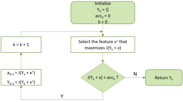
Figure 2.3: Fluxogram explaining the Sequential Forward Feature Selection algorithm

This algorithm is represented in the fluxogram in figure 2.3 and is described by the following steps:

1. Start with an empty feature setY0={}, an accuracya0= 0, an objective functionJ

andk= 0;

2. Select the featurex+that maximizesJ(Yk+x);

3. IfJ(Yk∪ {x+})> ak, updateYk+1=Yk∪ {x+},ak+1=J(Yk∪ {x+}) andk=k+ 1 and go back to2., otherwise continue;

4. Keep only the feature setYkand discard the rest.

The objective functionJ is a function that returns a value that quantifies the perfor-mance of the algorithm. In the present work we chose to use accuracy computed with 10-fold stratified cross-validation.

2.1.5 Validation

After a classifier has been trained, its performance must be evaluated. This is usually done by testing the resulting classifier on a dataset and observing if the resulting predictions match the original labels.

We cannot, however, use the same data we used in training for testing. Even though if the algorithm correctly classifies the data it was trained on, the classifier could show poor performance when shown new data. This is because the model might be overly

(32)

adapted to the examples presented, and thus unable to properly generalize. To this we call overfitting.

To prevent the effects of overfitting from showing in the validation phase, we must

come up with more clever ways to make use of our dataset. To this end we recur to cross-validation, where part of the dataset is used to train the classifier and the other part is used to test it. There are multiple methods of performing this:

• Holdout method:An arbitrary percentage of samples is randomly assigned to the training set, while the remaining is used for testing. The training set is usually larger than the testing set.

• K-fold cross-validation:The dataset is randomly split into K equal sized subsets or folds. For i < K, the i-th fold is used for testing and the remainder data for training.

• Stratified K-fold cross-validation:Similar to K-fold cross-validation, but each layer has approximately the same ratio between classes as the full dataset. This is done to prevent class imbalance in each fold.

• Leave-One-Out cross-validation: Similar to K-fold cross-validation, but with K equal to the number of folds. This results in folds with single samples each.

• Leave-One-Group-Out cross-validation:Once again similar to K-fold cross-validation, but the folds are separated according to metadata such as the day of recording, user, position,etc.

To visualize the classifier’s performance it is common to use aConfusion Matrix. This is anN×N matrix where the number in position (i, j) corresponds to the number of sam-ples labeled as classi predicted as classj. Therefore, the number of correct predictions will be equal to the sum of the values positions wherei=j. The accuracy rating can be obtained according to the following expression:

accuracy =number of correct predictions

total number of samples (2.6) Another way to represent data is to divide each row in the confusion matrix by its sum. In this case the number in position (i, j) corresponds to the proportion of samples labeled as classipredicted as classj. This is called aNormalized Confusion Matrix.

2.2 Sound Analysis

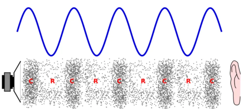
Sound is a vibration that consists on the propagation of pressure waves along a transmis-sion medium that can be either solid, liquid or gaseous. When propagated over a liquid or gaseous medium, such as air, the vibration is longitudinal to the propagation. This creates regions of compression, where the pressure is higher, and rarefaction, where the pressure is lower.

(33)

2 . 2 . S O U N D A N A LYS I S

An audio signal can be obtained through means of a microphone, a transducer that converts these sound waves into an electrical signal proportional to the pressure. Figure

2.4 illustrates a comparison between a sound wave and its representation as an audio signal.

Figure 2.4: Comparison between a sound wave and its representation as an audio signal. Below is the propagation of a sound wave where the dots represent air particles, C zones of compression and R zones of rarefaction. Above is the representation of this sound as an audio signal. (How to cite image from wikimedia commons?)

The electrical signal obtained from a microphone is continuous. However, a computer can only store and process discrete data, meaning we have to quantize the signal as in figure2.5. Quantization is the process of mapping a signal from continuous to discrete values both in time and amplitude, returning a discrete signal. Quantization in time is characterized by the sampling frequency, which indicates the number of values per second, and the quantization in amplitude is characterized in bit-depth, which defines the number of bits required to represent all possible values.

0 100 200 300 400 500 600 700 800 900

Time (μs) 000

001 010 011 100 101 110 111

Va

lue

in

bi

na

ry

Figure 2.5: Quantization of a continuous signal. The bit depth is 3 bits and the sampling rate is 10000 Hz.

(34)

2.2.1 Frequency Domain

Our human auditory systems do not distinguish sounds by their waveforms but by the frequencies they contain over a short period of time. For any discrete signal, the maximum frequency it can represent is the Nyquist frequency, given by half the sampling frequency [25].

The frequencies a signal contains can be represented by a power spectrum. For a discrete signalx[n] withN values, this can be obtained by the following expression:

P[f] = 2

N2 N X n=0

x[n]e−2πif n_/fs 2 (2.7)

Wherefsis the sampling frequency andP[f] the power for frequencyf in Hertz up to the Nyquist frequency.

2.2.2 Mel Frequency Scale

If we look at a common audio power spectrum, we can observe that most energy seems to be confined to the lower frequencies. As such, the human auditory system evolved to per-ceive pitch in a logarithmically rather than in a linearly, allowing it to better diff_erentiate

frequencies in the lower registers. We can easily perceive this in musical pitches: while we perceive the difference between two notes an octave apart as constant, the rising of an

octave actually represents a doubling in frequency.

The mel scale [24] is a scale that translates frequencies on hertz to how auditory systems perceive pitch. This is achieved by applying a logarithm with base two, thus assuring that the difference between octaves remains constant. This scale is normalized

in such a way that it maps the values of 0 Hz and 1000 Hz to 0 mels and 1000 mels, respectively. The conversion from hertz to mels is done by the following equation:

m= 1000×log2

1 + f 1000

(2.8)

Wheremis the pitch in mels andf is the frequency in hertz.

2.2.3 Audio Features

Given the first step in our machine learning algorithms return power spectrum, in the present work we chose to use features from the frequency domain, explained in more detail in the following subsections.

2.2.3.1 Logarithm of each frequency

In signal analysis and processing it is common to use decibels [19] (dB) to better represent and compare the power of sound signals. The logarithmic nature of the decibel allows bet-ter differentiation between values spread out different orders of magnitude. The formula

for translating a power to decibels is described by the following equation:

(35)

2 . 2 . S O U N D A N A LYS I S

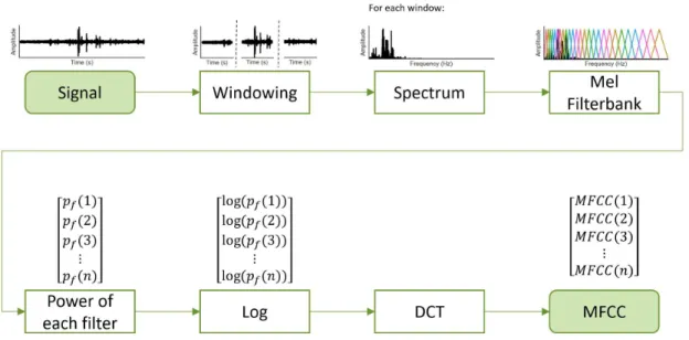
Figure 2.6: Diagram explaining how to computeMFCC.

P(dB) = 10×log(P

P0) (2.9)

WhereP is the power of each frequency in the spectrum, andP0is a reference power.

Common values for this reference include the threshold of human hearing for sound (dBA) and the value of one volt for electronically transmitted signals (dBV).

From equation2.9, the division of the intensity by a reference value and posterior multiplication of the logarithm by 10 will only result in a shift in mean and standard deviation, respectively. Since all features are normalized and given the lack of a reference, we chose to take only the logarithm of the power for each frequency.

2.2.3.2 Mel Frequency Cepstral Coeffi_cients

TheMFCCare a group of features commonly used in speaker [14] and speech recognition [29]. These have also been used in recognition of human activities based in recorded sound [7].

To compute the MFCCfrom the obtained power spectrum, we start by applying a filter bank of triangular overlapping windows whose frequencies are equidistant in the mel scale. Then a discrete cosine transform is applied to the logarithms of the sum of all values in each frequency band. This process is illustrated in figure2.6. The discrete cosine transformX(k) is given by:

X(k) = N−1

X

n=0

x(n)cosπ N

n+1 2

k (2.10)

(36)

2.2.3.3 Additional Spectral Features

Other type of common features used in audio analysis are the spectral features [20]. These features were also extracted from the background frequency spectrum. Definingf[n] the frequency corresponding to the nth _{bin and}_P_[_f_{] as its respective intensity, the following} features were calculated:

• Centroid: The barycenter of the spectrum, and it is computed by the 1st _order moment:

µ=

P

nf[n]·P[n]

P

nP[n]

(2.11)

• Spread: The variance of the spectrum around its centroid, and it is computed by the 2nd _{order moment:}

σ2=

P

n(f[n]−µ)2·P[n]

P

nP[n]

(2.12)

• Skewness: Gives a measure of the asymmetry around the centroid, and it is com-puted by the 3rd _{order moment:}

m3=

P

n(f[n]−µ)3·P[n]

P

nP[n]

(2.13)

• Kurtosis: Gives a measure of flatness of the spectrum, and it is computed by the 4th order moment:

m4=

P

n(f[n]−µ)4·P[n]

P

nP[n]

(2.14)

• Slope: Represents the amount of decreasing of the spectral amplitude, and it is computed by its linear regression:

slope=P 1

nP[n] ·N

P

nf[n]P[n]−Pnf[n]PnP[n]

NP

nf2[n]−(Pnf[n])2

(2.15)

• Decrease: Also represents the amount of decreasing of the spectral amplitude, and its formulation comes from perceptual studies, correlating to human perception:

decrease=P 1

n=1:NP[n]

· X

n=2:N

P[k]−P[0]

k−1 (2.16)

• Roll-Off: The frequency so that 95% of the signal’s energy is contained below this frequency. This frequency must satisfy the following condition:

f[k] : k

X

n=0

P[n]≥0.95·

∞

X

n=0

P[n] (2.17)

(37)

C

h

a

p

t

e

r

3

P r o p o s e d F r a m e w o r k

3.1 SoundSignature: Indoor Location based on Background

Spectrum Analysis

Every location has its own distinct set of constant background noises. These may have multiple origins, such as the humming of air conditioning systems, the noise of cars passing or a nearby road or the chirping of birds by the windows.

These background sounds are further modulated by the locations physical properties such as dimensions, materials used in its construction and placement of objects such as rugs and wooden furniture. These characteristics determine the location’s impulse response, which is the result of the echoes produced by an unit pulse in said location and acts as a filter for any sound produced in it.

Given these properties, we assume that each room has acoustic characteristics that are sufficiently constant and unique for identification. The algorithm proposed in this

chapter consists of a classifier makes use of these characteristics to predict the location the user is most likely to be in, from a set of previously recorded places.

The structure of the resulting algorithm can be seen in figure3.1.

Figure 3.1: Schematic representation of the SoundSignature algorithm.

(38)

C H A P T E R 3 . P R O P O S E D F R A M E WO R K

0 2 4 6 8 10

Time (s) 0 500 1000 1500 2000 2500 3000 3500 4000 Fre qu en cy (Hz ) Spectrogram −150 −100 −50 0 50 100 Int en sity (d B)

Figure 3.2: In this spectrogram of an segment of audio data we can visually discriminate two distinct components: a background noise spectrum that remains constant throughout the signal and transient sounds of larger intensity that are addictive to this spectrum.

3.1.1 Acoustic Fingerprint Extraction

Given an audio recording labeled with the location it was recorded in, we start by di-viding it into non-overlapping windows oftwinlength. Then we proceed to compute its spectrogram, which is a representation of the frequency spectrum as it varies with time. This is achieved by:

1. Divide the segment into frames oftf rame length;

2. Multiply each segment by a window function to reduce the signal’s amplitude near the boundaries, reducing some possible high frequency artifacts;

3. Compute the power spectrum for each frame;

4. Remove the redundant second half of the result;

5. Merge the result of each frame into a bidimensional map, resulting in a representa-tion of the signal’s power for a given frequency at a given time.

As shown in the spectrogram from figure3.2, two distinct components can be identi-fied in the spectrogram:

• Thebackground noise spectrum, that relates to the aforementioned intrinsic acous-tic characterisacous-tics of the location. This spectrum remains consistent throughout the spectrogram.

• Transient sounds, which are the cause of limited duration events such as speech or the sound of a door closing. These are always addictive to the background noise spectrum.

(39)

3 . 1 . S O U N D S I G N AT U R E : I N D O O R L O CAT I O N BA S E D O N BAC KG R O U N D S P E C T R U M A N A LYS I S

To separate this background frequency from the remaining sounds we could extract the minimum of each frequency along the spectrogram and merge them together to create a spectrum. However, this method is prone to errors due to a number of reasons:

• Common smartphone’s sound recording systems typically have some inherent dy-namic audio compression, which means that the larger the input signal, the lower the gain. This leads to dips in the signal’s gain following the recording of loud noises, causing readings with lower intensity than it is supposed to be.

• Electronic noisemay also lead to recorded intensities lower than expected.

Therefore, we instead extract the 5th percentile of each frequency, which is the value below which 5% of the observations may be found. This value is chosen because it is close to the minimum while being more robust to these effects.

The result is a spectrum that only contains information related to the background noise spectrum, and thus is aff_{ected only by the aforementioned acoustics characteristics.}

Therefore, we can use this spectrum as an acoustic fingerprint.

The extracted acoustic fingerprint consists of a power spectrum, making impossible the extraction of features in both the time and statistical domain. As such, we proceed to the extraction of the features described in section2.2.3, which are all in the frequency domain. These features consist of three groups: logarithms of the power for each frequency,MFCC

and additional spectral features.

All features were standardized according to equation2.1.

The best features are selected using the Forward Feature Selection described in section

2.1.4.

A classifier algorithm is an algorithm that maps input data to a category. It does so by generating a model from a training set containing observations whose category is known. It is on the basis of these that supervised learning are built upon.

There are multiple classifier algorithms. The choice of the algorithm will depend on various parameters such as the kind of data, number of observations and number of individual categories. In the present work, we chose to useSVM, as it was the most prevalent in the reviewed literature. This algorithm is described in detail in section

2.1.3.1.

When extending the algorithm to multiclass problems, there are two options: OvR

andOvO. While the first approach implements a smaller number of classifiers and has

(40)

therefore better computational performance, the resulting class imbalance between posi-tive and negaposi-tive samples in each classifier usually leads to worse results. As such, in the present work we chose to use theOvOapproach.

3.1.4 Validation

As explained in section2.1.5, using the same dataset for both training and testing may lead to overly optimistic results because of overfitting. To prevent this it is common to validate classifier algorithms resorting to cross validation.

In the present work, we used a common cross-validation method: K-fold cross-validation. This method randomly splits the data into K folds and creates K classifiers. Each classifier uses a different layer for testing and the remaining K-1 layers for training. The estimated

accuracy of the classifier is equal to the average of the K classifier’s accuracy. Likewise, the confusion matrix can be obtained by summing all the resulting confusion matrices.

3.2 SoundSimilarity: Proximity Detection from Real-time

Comparison of Audio Signals

In section 3.1, we studied how we can recognize a device’s location by examining the sound perceived by its microphone. In this section, we develop a tool for further improv-ing the proposed positionimprov-ing algorithm by comparimprov-ing in real time the sounds received by various users.

If the sound perceived by two users is similar, we can assume they are in the same location. Therefore, if the locations predicted by the SoundSignature algorithm for each user are different, we conclude that at least one of them is wrong. By comparing the

pre-diction probabilities of each user we can identify which prepre-diction is wrong and correct it.

As such, the objective of the SoundSimilarity algorithm is to develop a binary clas-sifier that identifies whether two sounds are similar. To achieve this we developed a novel measure of similarity between the sounds recorded by two different devices. Such

measurement must have the following properties:

i) Havepositive correlation with similaritybetween a pair of signals, meaning that the more similar are the signals, the larger will this measurement’s value be;

ii) Immune to small time misalignments, as it is diffi_{cult to perfectly align signals}

from different devices in real time;

iii) Immune to phase diff_erences, as different positions in the same locations may

per-ceive different sounds in different phases;

iv) Allowcomparisons between sounds from diff_{erent devices};

(41)

3 . 2 . S O U N D S I M I L A R I T Y: P R OX I M I T Y D E T E C T I O N F R O M R E A L-T I M E C O M PA R I S O N O F AU D I O S I G N A L S

v) Given this algorithm is meant to correct possible mistakes from the SoundSignature algorithm, any sort of training on the same previously recorded data could lead to the same errors. Therefore, the proposed SoundSimilarity algorithm must be

independent of any previous knowledge.

Figure 3.3: Schematic representation of the SoundSimilarity algorithm.

3.2.1 Cross-Correlation

In order to evaluate the similarity between two recorded audio signals, a cross-correlation was used. Cross-correlation can be defined as measure of similarity between two series as a function of the displacement between them. For two real valued discrete signalsf[n] andg[n], it can be formulated as:

(f ⋆ g)[n] =

∞

X

m=−∞

f[m]g[m+n] (3.1)

Given the finite length of the data, common practice is to extend the series with leading and trailing zeros. However, this method is prone to errors due to the resulting tendency to give more weight to central values, where these zeros do not interfere with the result. Therefore, we instead employ circular cross-correlation, where the input series are extended with periodic summations as in figure3.4.

Given the discrete-time Fourier transform already employs this extension, we can em-ploy the cross-correlation theorem and formulate the discrete circular cross-correlation as:

(f ⋆ g)[n] =F−1{F∗[f]·F[g]}[n] (3.2)

Where Frepresents the discrete-time Fourier Transform, F∗its complex conjugate andF−1the inverse discrete-time Fourier Transform. This formulation both avoids the

aforementioned artifact and greatly improves computational performance.

(42)

C H A P T E R 3 . P R O P O S E D F R A M E WO R K í í 7LPHV í í $PS OLW XG H 2ULJLQDOVLJQDO

(a) Original signal.

í í 7LPHV í í $PS OLW XG H 3HULRGLFVXPPDWLRQ

(b) Signal with periodic summation.

Figure 3.4: Illustration of periodic summation. This process consists of taking a signal limited in time and repeating it from−∞to∞, creating a periodic signal.

3.2.2 Measuring the Similarity of Audio Segments

Given the circular cross-correlation between two finite series, the series will be similar if a pronounced peak is present, as illustrated in figure3.5a. As such, we propose a novel measurement for audio similarity (MAS) correlated to the presence of a peak.

í í 7LPHGLVSODFHPHQWV í í í f⋆ g

(a) Signals recorded in the same location.

í í 7LPHGLVSODFHPHQWV í í í f⋆ g

(b) Signals recorded in different locations.

Figure 3.5: Comparison between two cases for circular cross-correlation of audio signals recorded at the same time.

Letf andg be two series corresponding to the recordings of two microphones in a window oftwinlength. Assume the misalignment in time between them istdelay< twin/d, whered is a free parameter. Given a circular cross-correlationCf ,g between these two series, we start by taking the absolute value of each value in the correlation:

Cabs=|Cf ,g| (3.3)

Then we define a regionRcentered aroundtwin/2 and with widthtwin/d:

(43)

3 . 2 . S O U N D S I M I L A R I T Y: P R OX I M I T Y D E T E C T I O N F R O M R E A L-T I M E C O M PA R I S O N O F AU D I O S I G N A L S

R= [twin 2 −

twin 2d ,

twin 2 +

twin

2d ] (3.4)

Finally, we define theMASas:

MASf ,g= 1−min(

max_t_∈_RCabs

maxCabs ,1) (3.5)

If a pronounced correlation peak is present, it will be contained in the regionR. There-fore, the overall maximum of the correlation will be larger than the maximum inR, the re-gion complementary toR. The greater this difference the closer to zero the ratiomaxt∈RCabs

maxCabs

will be.

On the other hand, if no correlation peak is present, we can suppose that the corre-lation has the properties to those of noise. In this case, two situations can occur: if the overall maximum is contained inR, we can obviously say that it is equal to the maximum inR, and therefore the ratio between them will be one; if the overall maximum is con-tained inR, it will be approximately equal to the maximum inR, and therefore the ratio between them will be approximately one. These regions are depicted in figure3.6.

Figure 3.6: Graph of the absolute values of a correlation with a peak, normalized to [0,1].

MASf ,gwill be equal to the maximum inRminus the maximum inR.

Given these properties, the result of this measurement is a value between 0 and 1 where the greater the value, the more similar are recorded sounds used as input. Further-more, by defining a range where the correlation peak can be instead of a fixed point, we make the algorithm robust to small misalignments in time and phase shifts.

If we divide two aligned audio signals into windows of equal length and compare those that correspond to the same time interval, we can obtain a graph of audio similarity along time. While the resulting graph allows to visually determine when the compared microphones were in the same location, we can observe some high frequency artifacts. To remove these we employ a low pass filter to smooth the signal. The comparison between before and after filtering can be observed in figure3.7.

(44)

C H A P T E R 3 . P R O P O S E D F R A M E WO R K 7LPHV M A Sf, g

(a)MASf ,g before filtering.

7LPHV M A Sf, g

(b)MASf ,g after filtering.

Figure 3.7: Graphic of theMASover time between two signals and comparison between before and after filtering.

3.2.3 Binary Classification

Obtained a measurement of similarity that satisfies the requirements in section3.2, we proceed to build a binary classifier from it. The simplest method is to apply a threshold value. If the measurement of similarity is greater than this value, the sample will be classified as positive and we consider that the two compared devices are in the same location. Otherwise, the sample will be classified as negative and we consider that the two compared devices are in diff_{erent locations.}

3.2.3.1 Sensitivity and Specificity

When building a binary classifier from labeled data there are multiple metrics that can be extracted. Two of these are sensitivity andspecif icity. Sensitivity determines the probability that a labeled positive sample is classified as such and is defined by:

sensitivity=T P

P (3.6)

WhereT P is the number of positively labeled samples classified as such andP is the total number of samples labeled as positive.

Similarly,specif icityrefers to the probability of a sample labeled as negative being classified as such. It is defined by:

specif icity=T N

N (3.7)

WhereT N is the number of negatively labeled samples classified as such andN is the total number of samples labeled as negative.

(45)

3 . 3 . AC T I V I T Y M O N I T O R I N G

3.2.3.2 Receiver Operating Characteristic curve

Varying the threshold affect both sensitivity and specificity: higher values increase

speci-ficity, while lower values increase sensitivity. To visualize the the trade-offbetween these

effects we plot the_sensitivity against 1₋_{specif icity}. This is called aROC.

Youden’s J statistic is a performance metric extracted from theROCcurve that is equal to the probability a correct classification. In the plot of aROCcurve, Youden’s J statistic for a certain threshold is equal the vertical difference between theROCand the diagonal

random chance line, as represented in figure 3.8 and it is calculated by the following equation:

J=sensitivity+specif icity−1 (3.8)

We choose the threshold that maximizes Youden’s J statistic. If a measurement is above this threshold, the devices are in the same location. If a measurement below this threshold, the devices are in different locations.

0.2 0.4 0.6 0.8 1.0

1−specificity

0.0 0.2 0.4 0.6 0.8 1.0

se

nsi

ti

vi

ty

J

ROC curve

ROC curve Random guess

Figure 3.8:ROCcurve depicting Youden’s J statistic.

Another performance metric that can be extracted from theROCcurve is theArea Under the Curve (AUC). This metric is equal to the probability that a classifier will rank a randomly chosen positive instance higher than a randomly chosen negative one (assuming "positive"ranks higher than "negative"). It varies between 0.5 and 1.0 and is used when determining if a measurement is suitable for a certain binary classification problem (the greater the value, the more suitable is the measurement).

3.3 Activity Monitoring

Similarly to the SoundSignature algorithm described in section3.1, the objective of the algorithm described in this section is to learn from labeled audio data how to classify

(46)

future inputs. However, instead of identifying the location the user is in, this algorithm recognizes everyday activities such as brushing teeth, talking and watching television. As such, the proposed algorithm is focused in the field ofHAR.

Many activities are location dependent. Brushing teeth, for example, is an activity typically done in a bathroom, and the capturing the sound of a television indicates prox-imity to said object. This allows the algorithm to be used in conjunction to the other two previously described algorithms for indoor location.

Given that the SoundSignature algorithm already implements a sound-based machine learning architecture, we chose to reuse it in the context ofHAR. The only diff_{erence in}

its implementation lies in the first step, the acoustic fingerprint extraction explained in section3.1.1.

Figure 3.9: Schematic representation of the activity monitoring algorithm.

3.3.1 Preprocessing

In the case of identifying locations, the first step was to isolate the background noise from sounds of limited duration. However, in many cases the sound derived from an activity has exactly this property of being limited in time, and as such by applying this fingerprint extraction the information relative to the activity would be lost. Because of this, only the power spectrum is extracted from each window. This permits the segmentation of the signal into shorter window, allowing the extraction of more samples from our data. The signal was therefore split into windows of 0.1 seconds from which the power spectra are extracted.

As in the SoundSignature algorithm, three groups of features were considered: the loga-rithm of the power of spectra,MFCCand additional spectral features.

The increase in the amount of samples made the implemented feature selection algo-rithm unusable due to the computational power needed. As such, the groups of features were tested separately.

(47)

3 . 3 . AC T I V I T Y M O N I T O R I N G

As in the SoundSignature algorithm, the chosen classifier algorithm wasSVM. The choice was made based on its prevalence in the reviewed literature.

To compensate for the loss in computational performance derived from the increase in samples, the chosen strategy for extending the algorithm to a multiclass problem was

OvR.

3.3.4 Validation

When extracting multiple samples from the same audio recording, it is expected that these will be more similar between them than samples from diff_{erent recordings. Because}

of this, a variation on the 10-fold stratified cross-validation was implemented:

1. Split the audio recordings into 10 groups, each with equal amount of recordings of each class;

2. In each group, segment the recordings into samples of 0.1 seconds and extract the desired features;

3. Use the resulting groups as folds for the regular 10-fold cross-validation algorithm.

(48)

(49)

C

h

a

p

t

e

r

4 R e s u lt s

To validate the proposed algorithms, separate datasets were recorded or downloaded from the Internet.

4.1 SoundSignature

4.1.1 Proof of Concept

In a first approach, a small dataset was recorded to function as a simple proof of concept. This dataset consisted of several audio recordings where the recording device would just stay in the same place for 60 seconds, either in the hand of the user or laying in a flat surface. The locations chosen consisted of physically distinct rooms such as an offi_{ce or a}

balcony.

Each recording was labeled with a tag indicating the place it was recorded in and split into 5 second windows to be used with the previously described algorithm. Table 4.1

shows the label of each recorded place and the number of 5 second windows recorded.

Table 4.1: Composition of the dataset used for proof of concept.

Location Number of windows

office 31

hallway 30

entryhall 20

restaurant 17

livingroom 9

openspace 8

restaurant_balcony 3

Total 125