DOI: http://dx.doi.org/10.1590/1806-9126-RBEF-2018-0190 Licença Creative Commons
BOVESPA: Stochastic or Deterministic?
Diógenes Borges Vasconcelos
1, Adriano Pereira Guilherme
2, Sandro Ely de Souza Pinto
*3 1Universidade Tecnologica Federal do Paraná, Departamento Acadêmico de Física, Curitiba, PR, Brasil2Universidade Federal do Amazonas, Instituto de Saúde e Biotecnologia de Coari, Manaus, AM, Brasil 3Universidade Estadual de Ponta Grossa, Departamento de Física, Ponta Grossa, PR, Brasil
Received on June 22, 2018; Revised on September 30, 2018; Accepted on October 31, 2018.
We aim to present an interdisciplinary way of showing the subject determinismversusstochasticity; and write the text in such a way that this subject can be treated from the point of view of physics teaching. We approach the technical part of this work intuitively and later we present this question in a more formal way. When the trajectory of a dynamical system in the phase space repeats itself after some time. We say that the system displays recurrence. Recurrence plots (RP) and recurrence quantification analysis (RQA) took place as tools to investigate this property. We employ the RP and the RQA the behavior of a long time series of the returns of the Bovespa index. We have carefully studied the obtention of the parameters for the phase space reconstruction of the supposed dynamical system which created the time series. After building the RPs for the time series of the returns, the values of the quantities from RQA were computed and then compared with values obtained for the randomized series. Our investigations suggest that the real financial market dynamics is a combination of deterministic chaos and stochastic behavior.
Keywords:Stockmarket; Stochastic; Determistic; Recurrence Plots.
1. Introduction
In a simplified way, the role of a scientist is to observe a system and explain it in order to translate such explana-tions into a mathematical form. Through this mathemati-cal model, it is possible to reproduce the observed system behavior, in order to facilitate the theoretical examina-tion and the speculaexamina-tion about the temporal evoluexamina-tion of the system, besides the prediction of new phenomena. In this work, we consider two types of mathematical models: the deterministic and the stochastic ones. The former manages to establish a temporal evolution that repeats itself if we always use the same set of initial conditions. The latter depends on a probability density function, and it is not possible to always retrieve the same result when we start with the same set of initial conditions. From the point of view of physics teaching, we feel the lack of literature that addresses the difference between determinism and stochasticity. For this reason, we have decided to write this manuscript, to try to fill this gap a little bit. We choose to examine a system that draws at-tention in the real world because it moves a large amount of money and knowing how to model such a system is the dream of many people. This system is the financial market. In these notes, we will scrutinize a component of the financial market, the Stock Exchange of the State of São Paulo.
Some physicists consider the financial market as a com-plex system, which presents real problems that deserve
*Endereço de correspondência: [email protected].
truncated Levy flight. The detection of long-range corre-lations in the Bovespa index appears as a result of the reference [22]. The authors of the reference [23] present an introductory course to econophysics. Finally, among other works, reference [24] presents a quantification of fluctuations in the Brazilian stock market.Here we do not treat with stochastic processes and Poincaré returns, and we do not deal with the chance of people gain or lose money under certain a probability. Instead, we are interested in understanding the mechanisms that govern the stock market index returns from a deterministic point of view, using the return map of the stock returns.
We organized the article as follows. To ensure a quick apprehension of the reader of the primary theoretical tool used in this work, we have graphically introduced the concept of return plot in Section 2 of this paper. Sub-sequently, the manuscript becomes more technical, but the question about the difference between determinism and stochasticity permeates the whole discussion that is in the text. In Section 3 we present briefly the Brazilian stock market index, or Bovespa Index, which is the focus of our study. Section 4 makes an overview concerning phase space, chaotic attractors, and phase space recon-struction; we also accomplish the reconstruction of the Brazilian market attractor to estimate its fractal dimen-sion. In Section 5 we make an overview of recurrence plots (RP) and quantitative recurrence analysis (RQA). In section 6 we use the RQA based on the time series of Bovespa Index to suggest it has a deterministic compo-nent. In Section 7 we present some scaling laws obtained through the RQA. Finally, in section 8 we present our conclusions.
2. An intuitive approach to return plots
A significant part of the experimental data collected in the real world comes in the form of long time series. These series are analyzed using several techniques, but the pur-pose of the analysis is always the same: to understand the dynamic behind the process that generated this series, to establish a mathematical model based on some suitable variables and parameters, and then to use the model built for predict the dynamic at a future time. In general, the time series can be generated by a stochastic or determin-istic system. In the determindetermin-istic case, a system creates a sequence according to a rule. A notable example would be the trajectory described by a particle under the action of an external field. As we learn in classical mechanics once the forces acting on a particle are known, Newton’s laws allow us to understand the future motion from a given initial condition, that is, we can determine future states (the points of the trajectory) uniquely from the past states. In the case of a stochastic system the series arises without any previously established rule, we say in this case that the data are random: a typical realization of such a system is the flipping of a fair coin each day to determine the price of an asset on the next day. Anotherexample of a deterministic series is the one provided by the logistic mapxn+1=axn(1−xn), in whicha∈[0,4]
andx∈[0,1][26]. In this equation the state variable at timen+ 1,xn+1, obtained fromxn, is reintroduced into
the equation in order to generate a new state. In this way, we can generate a time series{x0, x1, x2, ...}from a certain initial conditionx0. A system which evolves ruled by this equation will exhibit a great dynamic diversity, according to the value of the parameter a: stationary solutions (fixed points), cycles, aperiodicity (chaos). In Figure 1(a), we represent a small fragment of a long time series generated by the logistic map whena= 3.83, we can see that the dynamic is that of a cycle of period
Figure 1:(a) Logistic map time series witha= 3.83and 200
instants. (b) Recurrence plot for the series in (a). (c) Logistic map series witha= 4.00and 200 instants. (d) Recurrence plot
3, that is, {0.505,0.957; 0.156; 0.505; 0.957;...}. In this case, the system described by this equation returns to the same state every three iterations. This return of the system to a certain state or even a neighborhood of this state is known as recurrence. A graphic way to see this recurrence would be to construct the recurrence plot, see Figure 1(b): in this type of graph, we compare the value of the variable x at a certain instant i with its value at another instantj. We repeat the same procedure for all other points in the analyzed series. Every time the values of the variables associated with two instantsiand j are within a small neighborhood ε we draw a black dot in the coordinates(i, j)of a graphiversusj, if the points are outside this neighborhood, we draw a white point. We will formally introduce this type of graph into a future section, but we can already mention some of its striking features. In Figure 1(b) we notice the regularity in the spacing between the 45 degree inclined strips, this is a striking feature in an RP for periodic dynamics. In Figure 1(c), we show a logistic map series fora= 4.00, at first glance, the dynamic does not seem to differ much from stochastic dynamic (Figure 2(a)), but this is only apparent. The dynamic generated by the logistic map witha = 4.00 has exceptional characteristics: absence of cycles (aperiodicity), the dynamics is limited to the interval [0,1], the dynamic presents sensitivity to the initial conditions [26]. In this case, we say that the dy-namic is chaotic. It is interesting to compare the RPs for the chaotic series with the stochastic one (Figures 1(d) and 2(b)), we note two very striking differences, the RP for the chaotic series presents greater recurrence, it also shows a set of45degree inclined strips of various sizes,
Figure 2:(a) Random number time series in the interval [0,1] with 200 instants. (b) Recurrence plot for the series in (a).
the so-called diagonal structures. Such characteristics are not present in stochastic dynamics.
3. The Bovespa Index
The movements of the prices in a stock market reflect the changes in the business environment of a market or a sector of a market. These movements can be captured using stock indices, which express the performance of the stock prices of a collection of important companies in a market. The Bovespa index hereafter referred to as Ibovespa, is the main indicator variable of the Brazilian stock market [27]. For the analysis of such an index, represented in this work byI(t), we selected a dataset with 846,000 successive observations sampled each 30 seconds, from January 2003 to February 2007 (50months or1050trading days). Figure 3(a) showsI(t)as a function on timet. The visual examination of this figure shows us thatI(t)increases for time intervals of about20months. However, we can observe a decreasing behavior of the index for a shorter time interval, as illustrated in the small inset. This oscillation is one of the most studied features of the stock market indices since it is thus important to know if the index will increase or decrease after a time interval. This issue is about how much money people will gain or lose with the change of the stock market index at a period. A device for measuring changes in the stock market index is the return of this economic variable, defined by
Z(t)≡ln
I(t+δt)
I(t)
, (1)
where δt is an arbitrary time interval multiple of 30 seconds. In this work we shall useδt= 30s.
A more simplified version of that quantity is the stan-dard return index, which is defined by
z(t)≡Z− hZi
σ , (2)
where hZiandσare the mean value and the standard deviation of the distribution ofZ, respectively. The trans-formation (2) provides a distribution with mean value equals zero and standard deviation equals 1. Therefore, all fluctuations about the mean are measured in units ofσ. In figure 3(b) are displayed the dependence of the standard return index zon timet for the data used in 3(a).
4. Phase Space and Attractor
Reconstruction
Figure 3:(a) The IbovespaI(t)time series from January 2003
to February 2007. (b) Ibovespa standard returnzas a function on timetforδt= 30s.
~x(t) = (x1(t), x2(t), ..., xf(t))traces an orbit in this f
-dimensional space. In dissipative systems, the orbits are attracted asymptotically from a basin of initial condi-tions to a limiting set of states called attractor. The volume of an attractor is always zero and its dimension d typically smaller than the dimension f of the phase space. Despite these simple characteristics some attrac-tors can have very intricate structures [28]. A chaotic attractor, for instance, is a set of states on which the orbit wanders forever visiting regions of the phase space in a non-periodic and highly disordered way. Although the phase space of a dissipative system can be possibly high dimensional, the dynamics on the attractor is nev-ertheless low dimensional, in other words, the effective number of degrees of freedom needed to characterize the long-term dynamics is relatively small. The low dimen-sional feature is an advantage since we are particularly interested in studying the evolution of the attractor of a dynamical system itself and not the evolution in the full, high dimensional phase space. Following this idea, we suppose in this work that all-time series emerge from a chaotic attractor of a possible high dimensional system, the stock market itself.
In computer experiments we generally know the vec-tor state~xat each instant of time because we have the mathematical equations for the time evolution of~x, in other words, we have a model at hand. However, for natural experiments, the equations of the system under investigation is unknown, and consequently, we do not have access to all components of the vector~x, which can have thousands of components, but to only one or at
most a few components of it. However, such a situation does not represent, at least in a preliminary investigation, an obstacle to construct or model the dynamics on the attractor. Since a single-variable experimental time series from a system is affected by all of the state variables, it, therefore, contains some historical information of the dynamics. It is thus possible in principle to reproduce the dynamics from a single-variable time series without reference to other state variables. This single-variable approach is the central idea of the phase space recon-struction method. Packard presented this idea [29] from a purely empirical point of view, but it also has a rig-orous mathematical basis in the works of Whitney [30], Takens [31] and Mané [32]. We shall describe it below empirically by considering the time series of the Ibovespa standard returnz(t)as the single-variable natural time series obtained from the Brazilian market attractor.
Suppose the single-variable experimental time series {zn, n= 1, . . . , N, znR} ofN successive points on ad
-dimensional attractor (d≤f). In order to reconstruct the dynamics on the attractor we must transform the scalar measurementszn in vector states ~ξof a new m
-dimensional phase space. Each vector ~ξ consists of a m-tuplet of consecutive values (delayed coordinates) of the time series.
~
ξi= (zn, zn+τ, . . . , zn+(m−1)τ), (3)
where the delay timeτ is some multiple of the spacing between successive measurements.
When this set of vectors are graphed (embedded) in the newm-dimensional space, it can be analyzed as if it were an orbit of a dynamical system. Though the reconstructed attractor usually has a different shape of the original one, it preserves the original dynamical properties provided we determine an adequate value form.
If we choosemtoo small it may happen that the re-constructed attractor is too folded, that means that two distant points on the attractor in the original phase space will overlap each other in the reconstructed space. This overlapping of points, known as false-neighbors points, produces errors in the calculation of many dynamical properties since the calculation are based on the trajec-tories in the phase space. This overlapping can also be seen as a self-intersection of the reconstructed orbit at a given instant of time, which leads clearly to a violation of the deterministic nature of a trajectory: it is not possible to have two distinct future states from just one prior state (or initial condition). To disconnect these false-neighbors points, the attractor must be represented in spaces of higher dimensions. According to Takens Theo-rem,m= 2d+ 1is a sufficient condition for the attractor to be completely unfolded [33].
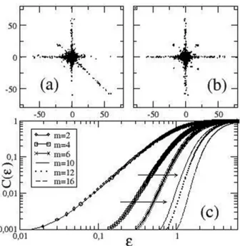
Figure 4: (a) Plane(zn, zn+1) of the reconstructed attractor from the Ibovespa standard return time series (δt= 30s). (b)
Plane(zn, zn+3)for the same dataset used in (a). (c) Correlation integralC(ε)versusthe thresholdεform= 2,4,6,10,12,16
andτ = 1. The arrows near the curve form= 10indicate the
limits of the linear scaling. We have used the first3000points
of the data set to compute each curve.
(or ball) of uniform scattered points, which is typical for data emerging from a random source, the set of points seems to have a strong spatial correlation. The straight horizontal or vertical lines appearing in Figure 4 are the results of a new zero return followed by a sharp increase, or decrease (or vice-versa) in return. These lines appear for the data collected at the opening and closing of the stock exchange. In these two times, the volume of transactions decreases and the Ibovespa variation is practically non-existent.
According to Takens theorem the required value for the embedding dimension mis known only if we determine the attractor dimensiond. A good estimation fordis the
correlation dimension dc [34]. To calculatedc we need
first evaluate thecorrelation integral,
C(ε) = lim
N→∞ 1 N2
N
X
i,j=1
Θ(ε− k~ξi−~ξjk), (4)
for the reconstructed orbit,N is the number of points on the attractor,εis a threshold distance,k. . .k is the Euclidean norm andΘ(.)is the Heavside step function. Grassberger and Procaccia established that for small ε the correlation C(ε) grows like a power, C(ε)≈εdc, and the exponentdc can be taken as a measure of the
dimension of the chaotic attractor [35]. It is clear that the obtained value for this exponet is affected by the choosed embedding dimensionm, since C(ε)itself is a quantity that depends on the distance between points in them -dimensional space. We conclude that if we calculatedc
by increasing m sucessively (m = 1,2,3, ...), once the attractor is fully unfolded dc must cease to modify as
mchanges, in other words,dc saturates. We have then
at the same time reached the exact value for dc and
m. On the basis of our assumptions we have estimate the correlation dimension dc for the Brazilian market
attractor as well as a satisfactory value form. Fig.4(c) presents the result, in this figure we can fairly observe a range of values ofεat which the slopedc (correlation
exponent) is constant, we have used this range to feet the power law scaling region. We can observe a reasonable saturation beyondm= 10(see table), we shall use the valuem= 10throughout this work. The corresponding fractional dimension calculated isdc≈6.004.
5. Recurrence Plots and Recurrence
Quantification Analysis
We saw that in a chaotic dynamical system the orbit exhibits bounded, aperiodic and highly erratic behavior. Though the state variables never return to their previous values, they may return very close to them. Recurrence plots (RPs) [36,37] provide a graphical representation of how close an orbit or a reconstructed orbit approaches or recurs itself, in other words, RPs exhibit the recurring patterns of a system. Such a graphical representation can be introduced by theN×N matrix
Ri,j= Θ(ε− kξ~i−~ξjk) i, j= 1,2, ..., N, (5)
where ~ξ∈Rmrepresents a dynamical state in them
−di-mensional phase space. The RP is thus obtained by as-signing a black dot, called recurrence point, to a position of coordinates(i, j) provided that the spatial distance between the system states at instantsn=iandn=j is smaller than a distance ε. The construction of RP
Table 1:Estimate of slopedc for different embedding dimensions, fromm= 2throughm= 12. We presume that form= 10a
saturation value fordc is attained.
m Estimated slopedc Standard deviation Correlation coefficient
requires the specification of the time delayτ, but for dis-crete time series such as financial data , τ= 1is usually apropriate. [42] [17].
The recurrence points (black dots) may form two small-scale structures which contribute to the overall pattern of the RP: the vertical and diagonal lines. A vertical line identifies a state which does not change considerably during an interval of time [38], the length of this interval is precisely the length of the vertical line. A diagonal line, represented by any line parallel to the main diagonal, identifies two similar segments of the trajectory beginning at different instants of time, the length of a diagonal line is the interval of time in which those distant segments remain similar. A priori, diagonal and vertical lines must not occur in a RP arising from a random time series [41].
Different time series exhibit different RPs; we have thus a huge number of visual patterns, which depend on particular details of dynamics. Introduced by Zbilut and Webber [39–41,43–45], therecurrence quantification analysis(RQA) assigns a group of real numbers to each RP regardless of its visual appearance. These numbers, or measures, were mostly based on the statistical analysis of diagonal structures, but a few years later, further mea-sures based on vertical structures have been integrated into this analysis [39]. The set of all measures represents a clear and sound criterion nowadays for comparison between RPs from different types of dynamics. Since RPs and RQA were introduced they have been exten-sively used in a wide diversity of applications: quantifi-cation of complex behavior in heart-rate-variability [38] and electroencephalographic data [47], quantification of correlation between data from different climatological phenomena [46]. More recently they were also extended beyond the domain of time analysis: the quantitative analysis of spatial disorder or correlation in complex spa-tial patterns at a fixed time [48,49]. In this work we deal with four measures, namely therecurrence rate (REC), the determinism (DET), the entropy (ENT), and the
laminarity(LAM) [38,43,44].
The simplest measure of the RQA is the recurrence rate
REC(ε) = 1 N2
N
X
i,j=1
Ri,j(ε), (6)
which is a measure of the density of recurrent points in the RP.
The laminarity is definded as the ratio of recurrence points forming vertical structures of lengthv, larger than vmin, to all recurrence points.
LAM =
PN
v=vminvP(v)
PN
v=1vP(v)
(7)
P(v)denotes the histogram of the vertical lines. The determinismDET is defined as the ratio of recurrence points that form diagonal structures of lengthl, larger
thanlmin, to all recurrence points (points belonging to
the main diagonal are always excluded), and reads
DET =
PN
l=lminlP(l)
PN
l=1lP(l)
, (8)
in whichP(l)is the histogram of diagonal lines of length l.Stochastic processes display absence of short diagonals
even for large values ofε, whereas deterministic processes
cause longer diagonals and less single, isolated recurrence points. Another measure based on the length of diagonal lines is the Shannon entropy of the probabilityp(l) = P(l)/Nl of finding a diagonal line of lengthl in the RP,
EN T =−
N
X
l=lmin
p(l) log2p(l), (9)
where Nl is the total number of diagonal lines.A RP
with large (small) diversity of diagonal lines renders a high (small) value forEN T, e.g. for uncorrelated noise
the value ofEN T is quite small, indicating low diversity
of diagonal lines. The measure EN T is thus inversely related to the amount of disorder (dynamical complexity) in the time series under analysis. In the present analysis we have usedlmin= 3 andvmin= 2.
6. RQA for original and shuffled
financial data
The shuffling of a data series does not affect its statistical distribution, measures like mean, variance and standard deviation are preserved. On the other hand, the shuffling affects the ordering of data, measures like correlation and recurrence are therefore strongly affected: the more the set is shuffled, the more uncorrelated it becomes. Since the RP and the measures of RQA are based on the recurrence, it is thus possible in principle to find out if a time series has a deterministic or random nature by shuffling the data and comparing the respective RPs and the results from RQA for the original afterwards and shuffled series: if the RPs and the measures from RQA are different for the original and shuffled data series, we may suppose there must be a deterministic component in the original series.
Figure 5:(a) The recurrence plot for the interval[1; 4800]. (b) The recurrence plot for the interval[150001; 154800]. (c) Recurrence
plot for the shuffled data corresponding to (a). (d) Recurrence plot for the shuffled data corresponding to (b). All intervals are obtained from the time series showed in Fig. 3(b).
Although the time series of the standard return index display highly disordered data, the RPs, on the other hand, display some interesting large-scale structures or “clusters” of recurrence points. Such clusters disappear in the RPs for the shuffled data. The RQA reveals a large decrease in all four measures when we compare the original and shuffled data 2. The qualitative and quantitative analysis shows that the consecutive returns from the stock market must not be considered a set of disconnected and random data.
7. Scaling laws arising from diagonal and
vertical lines
The RP for a periodic time series consists of a series of parallel stripes at 45degrees, with length decreasing from the length of the main diagonal line to the length of the shortest diagonal line at the lower-right corner of the RP. The vertical distance between two successive stripes is right the period. Following this idea, it is thus possible to obtain some information about the periodicity of a reconstructed orbit from an arbitrary dynamical system by analyzing the set of vertical blank gaps, also called recurrence times, in the corresponding RP. The following process can obtain the set of recurrence times: for each stateiof the horizontal axe we compute the number and the length of the vertical blank gaps by varyingj from1
toN, the number of states of the reconstructed series, then we equally varyifrom1 toN.
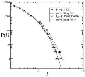
Once the set of recurrence times is obtained, we can compute the probabilityp(q)of finding a recurrence time of length q. We computed such a distribution for the RPs based on the intervalsI1andI2 studied in the last section. The empirical distribution, presented in figure 6 for both sets of recurrence times, can be exceptionally well fitted (see straight line) in the full range ofqby the mixed function
p(q) =α q−β
exp(−q/γ). (10)
Table 2:Measures of RQA based on RPs obtained from intervalsI1= [1,4800]andI2= [150001,154800]of the Ibovespa standard
return (δt= 30s).
RQA Original data Shuffled data ∆% %REC 1.18 0.103 −91.27 I1 %DET 69.67 39.837 −42.82 <|z|>= 0.496 %LAM 22.61 4.560 −79.83 EN T 2.889 1.820 −37.00 %REC 1.12 0.055 −95.09 I2 %DET 73.44 37.868 −48.43 <|z|>= 0.578 %LAM 30.92 3.954 −87.21 EN T 3.056 1.803 −41.00
Figure 6: Distribution of the recurrence epochs q, with q higher than 2, for the intervals (a) I1 = [1; 4800] and (b) I2 = [150001; 154800]of the Ibovespa standard return (δt= 30s). The straight line shows the fitting with the mixed function (equation 10).
we observed that the RPs for the corresponding shuffled data did not exhibit any recurrence pattern. As a result, the corresponding distribution of recurrence times must approximately follow a uniform distribution, and scaling laws will thus obviously not arise.
Motivated by the obtention of a simple function de-scribing the distribution of recurrence times, we also computed the probabilityp(l)of finding a diagonal line of lengthl from the RPs based on the intervalsI1and
I2. These distributions, with length llarger than3, are displayed in figure 7. Again, the fitting with a mixed function,
P(l) =α l−β exp(−l/γ) (11)
with parameters(α;β;γ) = (22767.20; 0.419; 3.272)forI1 and(α, β, γ) = (26048.4; 0.902; 4.949)for I2, showed to be remarkably good (see the straight and dashed lines). However, different from the distribution of recurrence times, a power law behavior extends only over a very small range. Moreover, we observe a quite small diversity of diagonal lines as well as the absence of long ones: the maximum value isl≈40, which represents a time interval of about only1200seconds (40 x 30s), in other words, the longest similar segments of the reconstructed series last
1200seconds. As for the corresponding set of vertical lines, we did not obtain a well-behaved distribution. Because of this, a fitting with some simple function was not possible.
The distribution of diagonal lines can be useful when we intend to accomplish a fast computation of the mea-suresDET andEN T, equations 8 and 9, respectively. A comparison between both ways of computation of these two measures is summarised in table 3. We see that the obtention ofDET andEN T by using equation 11 is in good agreement with the direct counting based on the RP, see the deviation presented in the last column.
8. Conclusions
This paper aimed to investigate whether there is some de-terministic behavior ruling the stock market. To do this
Table 3:Comparison between numerical and analytical results for RQA.
Numerical Analytical deviation % I1 %DET 69.67 72.40 3.92
EN T 2.889 2.885 0.14
Figure 7: Histogram of diagonal lines with length l > 3 for
the intervals I1 (◦) and I2 (). The corresponding fittings with equation 11 are also displayed: straight and dashed lines, respectively.
task, we have hypothesized the existence of a “hidden” dynamical system controlling a specific stock market, the Brazilian stock market. We have then applied the Grassberger-Procaccia method to estimate the dimen-sion of the attractor of the dynamical system. Different from data arising from a random source, the correla-tion integral computed for the dataset from Ibovespa tend to saturate around an embedding dimension of10 which leads to a fractal dimension of about 6.004. We laid a particular emphasis on the method of Recurrence Plots and Recurrence Quantitative Analysis; the broke of patterns in the recurrence plots and the decreasing of the measures from RQA after shuffling the dataset from Ibovespa support our hypothesis about the existence of a dynamical system.
We have analyzed the distribution of recurrence times and diagonal lines from the obtained RPs; both distri-butions showed to be extremely well fitted by a product of two essential functions: a power law and an exponen-tial function. This scaling seems not to depend on any particular segment of the time series.
Acknowledgments
We would like to thank BOVESPA for providing us with the data, without which it would not be pos-sible to carry out this work.Some numerical results displayed in this article were carried out with com-puter programs developed by Profs. Charles L. Web-ber Jr. and NorWeb-bert Marwan. These programs can be downloaded at http://homepages.luc.edu/∼cwebber and http://www.agnld.uni-potsdam.de/∼marwan. We would
also like to thank CAPES and CNPq for their financial support.
References
[1] B. Mandelbrot and R.L. Hudson, The Misbehavior of Markets: A Fractal View of Risk (Basic Books, Cam-bridge, 2004).
[2] R.N. Mantegna and H.E. Stanley,Introduction to Econo-physics: Corelations and Complexity in Finance (Cam-bridge University Press, Cam(Cam-bridge, 2007).
[3] J.P Bouchaud and M. Potters,Theory of Financial Risk and Derivative Pricing: From Statistical to Risk Manage-ment(Cambridge University Press, Cambridge, 2003). [4] J. Voit,The Statistical Mechanics of Financial Markets
(Springer, Berlin, 2005).
[5] R.N. Mantegna and H.E. Stanley, Nature376, 46 (1995). [6] P. Gapikrishnam, V. Plerou, L.A.N. Amaral, M. Meyer
and H.E. Stanley, Phys. Rev. E60, 6519 (1999). [7] P.C. Ivanov, A. Yuen, B. Podobnik and Y. Lee, Phys.
Rev. E69, 056107 (2004).
[8] M. Constantin and S.D. Sarma, Phys. Rev. E72, 051106 (2005).
[9] Z. Eisler, J. Prello and J. Masoliver, Phys. Rev. E76, 056105 (2007).
[10] H.E. Stanley and V. Plerou, Phys. Rev. E77, 037101 (2008).
[11] J.A. Holyst, M. Zebrowska and K. Urbanowicz, Eur. Phys. J. B20, 531 (2001).
[12] A. Krawiecki, J.A. Holyst and D. Helbing, Phys. Rev. E 89, 158701 (2002).
[13] A. Fabretti and M. Ausloos, Int. J. Mod. Phys. C5, 671 (2005).
[14] A.A.G. Cortines and R. Riera, Physica A 377, 181 (2007).
[15] A.A.G. Cortines, R. Riera and C. Anteneodo, Eur. Phys. Lett.83, 30003 (2008) .
[16] K. Guhathakurta, B. Bhattacharya and A.R. Chowdhury, Physica A389, 1874 (2010).
[17] J.A.S. Bastos, J. Caiado, Physica A390, 1315 (2011). [18] M.S. Baptista and I.L. Caldas, Physica A284, 349 (2000)
.
[19] M.S. Baptista, I.L. Caldas, C.S. Baptista, A.A. Ferreira and M.V.A.P. Heller, Physica A287, 91 (2000). [20] M. S. Baptista and I.L. Caldas, Physica A 312, 539
(2002).
[21] L.C. Miranda and R. Riera, Physica A297, 509 (2001). [22] R.L. Costa and G.L. Vasconcelos, Phsica A 329, 231
(2003).
[23] G.L. Vasconcelos, Braz. J. Physics34, 1039 (2004). [24] B.M. Tabak, M.Y. Takami, D.O. Cajueiro and A.
Peti-tiniga, Physica A388, 59 (2009).
[25] E.G. Altmann and H. Kantz, Phys. Rev. E71, 056106 (2005).
[26] K.T. Alligood, T. Sauer and J. Yorke,Chaos: An In-troduction to Dynamical Systems(Springer, New York, 1996).
[27] http://www.bovespa.com.br.
[28] E. Ott,Chaos in Dynamical Systems(Cambridge Uni-versity Press, Cambridge, 1997).
[30] H. Whitney, Ann. Math.37, 645 (1936).
[31] F. Takens, D.A. Rand and L.S. Young,Lecture Notes in Mathematics, (Springer-Verlag, Berlin, 1981).
[32] R. Mané, D. A. Rand, and L. S. Young, Lecture Notes in Mathematics, Vol.898, Berlin, Springer-Verlag, 1981, p. 230.
[33] H. Abarbanel, R. Brown, J.J. Sidorowich and L. Tsimring, Review of Modern Physics,65, 1331 (1993).
[34] P. Grassberger and I. Procaccia, Phys. Rev. Lett.50, 5 (1983).
[35] P. Grassberger and I. Procaccia, Physica D9, 189 (1983). [36] J.P. Eckmann, S.O. Kamphorst and D. Ruelle, Europhys.
Lett.4963 (1987).
[37] N. Marwan, M.C. Romano, M. Thiel and J. Kurths, Physics Reports438, 237 (2007).
[38] N. Marwan, N. Wessel, U. Meyerfeldt, A. Schirdewan and J. Kurths, Phys. Rev. E66, 026702 (2002). [39] N. Marwan, European Physical Journal ST, 164, 3
(2008)
[40] J.P. Zbilut and C.L. Webber Jr., International Journal of Bifurcation and Chaos17, 3477 (2007).
[41] J.P. Zbilut, C.L. Webber Jr. and A. Giuliani, Phys. Lett. A237, 131 (1998).
[42] J.P. Zbilut, in:Economics: Complex Windowseditado por M. Salzano and A. Kirman (Springer-Verlag, Mai-land, 2005), p. 91.
[43] J.P. Zbilut and C.L. Webber Jr., Phys. Lett. A171, 199 (1992).
[44] C.L. Webber Jr. and J.P. Zbilut, J. Appl. Physiol.76, 965 (1994).
[45] L.L. Trulla, J.P. Zbilut, C.L. Webber Jr. and A. Giuliani, Phys. Lett. A223, 255 (1996).
[46] N. Marwan and J. Kurths, Phys. Lett. A302, 299 (2002). [47] N. Thomasson, T.J. Hoeppner, C.L. Webber Jr. and J.P.
Zbilut, Phys. Lett. A279, 94 (2001).
[48] D.B. Vasconcelos, S.R. Lopes, R.L. Viana and J. Kurths, Physical Review E73056207 (2006).

![Table 2: Measures of RQA based on RPs obtained from intervals I 1 = [1, 4800] and I 2 = [150001, 154800] of the Ibovespa standard return (δt = 30s).](https://thumb-eu.123doks.com/thumbv2/123dok_br/16190244.709831/8.892.166.753.154.594/table-measures-based-obtained-intervals-ibovespa-standard-return.webp)