A Work Project, presented as part of requirements for the Award of a Master Degree in Economics from the NOVA – School of Business and Economics
BUBBLES IN THE EUROPEAN REAL ESTATE MARKET:
INTRINSIC OR RATIONAL SPECULATIVE?
HENRIQUE GUEDES NEVES DUARTE DE OLIVEIRA | 3110
A project carried out on the Master in Economics Program, under the supervision of: Professor Paulo M. M. Rodrigues
2
BUBBLES IN THE EUROPEAN REAL ESTATE MARKET: INTRINSIC OR RATIONAL SPECULATIVE?
Abstract
The purpose of this dissertation is to model the real estate market of four European countries (Spain, UK, Ireland and France), over recent years, to assess during which periods there was a deviation of the property price from its fundamental value, and whether these deviations are the result of unrealistic expectations about its future price, or from an overreaction to changes in fundamentals. A quantile regression and a Markov-switching model were performed, to conclude that for Spain and the UK unrealistic expectations predominated, whereas for France and Ireland an overreaction to changes in disposable income and rents lead to exuberant price behavior.
Keywords: House price; Rational Speculative Bubble; Intrinsic Bubble; Markov-Switching Model; Quantile Regression
3
1. Introduction
Real estate (houses) are the assets which weight most on households’ budgets, thus changes in the evaluation of such assets have immediate effects on their wealth, with repercussions on public consumption and on the credit channel. For these reasons, it is crucial to understand how property prices change with other variables, at a macroeconomic level, and what factors lead to an unexpected behavior regarding real estate price valuation.
Sometimes, and due to multiple reasons, asset prices (properties, stocks, bonds, etc.) may differ from their fundamental value, and when this misalignment occurs consistently over several periods of time, one may be in the presence of a bubble. Even though there are numerous types of different bubbles, they all share some common “big signs”, namely: rapid pace of movements, a lot of speculation without the proper understanding of the risks, and people who otherwise do not invest are looking to enter the market.
Bubble episodes are not that recent and may occur in all types of assets, not only to the most known, such as real estate or stocks. The oldest report about bubbles dates back to 1630’s, when tulips arrived at the Dutch Republic and its price was driven by the public’s enthusiasm to high levels, and its subsequent collapsed at begin of 1637. This episode was most known for the social phenomena, rather than for the economic consequences caused. However, the most dangerous thing about bubbles is that usually, one cannot understand whether the price evolution is due to pure speculation or not. The most recent example of this phenomena is the cryptocurrency: in spite of its parabolic price behavior and the lack of intrinsic value and rate of return, one cannot argue that it is for sure a bubble because it can be a future transactions trend.
Over the past years, countries worldwide, including European ones, have been concerned that exuberant price movements could emerge again, and bring some of the devastating impacts such as those originated by the collapse of the US Sub-Prime, back in 2007,
4
which lead to the most severe financial crisis of the last years. The real estate market is of special importance because, according to some researchers, most of the financial crises could be predicted using real estate data.
The ultimate goals of this dissertation are the determination of whether there is statistical evidence of bubbles in the European real estate market, and if this is confirmed, the modelling of the past years of exuberant price behavior across four European countries that most suffered from the 2007 US subprime collapse. In this analysis the separation proposed by Nneiji et al. (2013) which divided the bubble into rational speculative and intrinsic will be used, in order to understand whether bubbles result from unrealistic agents’ expectation about future asset prices (rational speculative bubbles), or from the overreaction of changes in macroeconomic determinants (intrinsic bubbles), such as disposable income and the rate of return (rents).
This dissertation is organized as follows. Section 2 briefly reviews the existing literature on this topic. Section 3 describes the real estate price data and the price-to-rent evolution over the time periods. Section 4 presents and explains the statistical methods used in this research. Section 5 introduces the main estimation results and section 6 draws the conclusions and drawbacks of this analysis.
5
2. Literature review
There are numerous studies which aim to analyze the relationship between real estate prices and macroeconomic variables. The main goal of such studies is to detect in which periods the real estate price was not in line with their macroeconomic fundamentals, and what is behind this behavior. Within the extensive literature about this topic, we can find several approaches. For example, some studies analyze the evolution of valuation ratios, such as, e.g., the price-to-rent and the price-to-income ratios (Poterba (1984), Gelain and Lansing (2014), among others); the inverse demand approach (Zhou (2010)); the log periodic power law singularity model (Ardila, Sanadgol and Sornette (2014)); as well as several other approaches.
The interest in modeling house prices results from their impact on the society and economy, and from the fact that houses fulfill individuals’ basic needs for shelter (Lu, 2016). Houses are the major part of a household’s wealth, thus changes in their prices can lead to changes in private consumption (Case et al, 2005, Chen, Gan, Hu and Cohen, 2012, Augustyniak et all, 2015, Kahn, 2008). Moreover, according to Kemme (2012), the financial crisis of 2008 could have been predicted using the evolution of the real house prices.
The main concern about the misalignment of prices is that it can be a sign of a speculative bubble. These bubbles (which are common for both real estate and stock markets) are composed of two different stages: first there is the “boom” period during which prices increase and there is a positive effect on economy; second when the bubble “bursts”, prices suddenly decrease and there is a negative effect on the economy. Normally this second stage is quicker than the former stage, it only takes a few weeks or months, and its negative effect is stronger than the positive effect of the first stage. Detken and Smets (2004) defined that an asset is in a “boom” when its market price is 10% above their fundamental price. Rodrigues and Lourenço (2015) argue that “bubbles arise when the expectations of future asset prices have an abnormally important influence on the valuation of assets”.
6
The most well-known bubbles episodes are the Wall Street Crash of 1929; the rise of real estate and stocks prices in the 1980s, for which Mankiw and Weil (1989), formulated a forecast model which argues that this rise was due to the Baby boom generation, which increased housing demand, when they entered the residential market; or the more recent US subprime market collapse of 2007 which Shiller (2008) argues was due to the fact that people did not know how to react to a speculative bubble.
Even though the literature about bubbles in the stock market is more extensive than for the real estate, Granziera and Kozicky (2013) treat houses as stocks, i.e., the house price being the stock price and the house rent being its dividend. Using a Lucas tree model with the assumption of rational expectations, they estimated the price and price-to-rent ratio evolution under these assumptions. Moreover, they relaxed the rational expectations assumption to evaluate the contribution of expectations in the real estate price formation and in the evolution of the price-to-rent ratio.
Although there are several common features with the stock market, the real estate market is very different from any other market. Ghysels et al. (2012) point out some distinctive characteristics, such as “large transaction costs, carrying costs, illiquidity, and tax considerations”. The impossibility of short-sale makes the “possibility of exploiting forecast decreases in property value” unfeasible. According to Fama (1970), these frictions make the real estate market much less efficient than the financial markets.
Also, Nneiji, Brooks and Ward (2013), as mentioned early, divided the type of bubbles into “Rational Speculative bubbles” and “Intrinsic bubbles”. Then applying a Markov-switching model to the price-to-rent ratio for the US between 1960 and 2011, they found that there was a switch from a regime of low price-to-rent ratios to high ratios in the years 2000. Furthermore, they argue that before 2000 the data suggests the existence of an intrinsic bubble with buyers overreacting to changes in rent prices. Regarding the observations after 2000, using
7
a separate test, there were indications of the emergence of a rational bubble that made the price-to-rent ratio increase, and reach its maximum value in the last quarter of 2005. Gelain and Lansing (2014) also studied the evolution of the price-to-rent ratio in the US between 1960 and 2013, not only allowing for risk aversion to vary over time, but also the persistence and volatility in the rent growth vary with time. Their main conclusion is that with rational expectations the volatility of the price-to-rent ratio is underestimated; but if agents are “near-rational”, i.e, give more attention to recent observations, the model can match the observed volatility. With a moving-average model only, the agent predicts high future returns when prices are relatively high regarding their fundamentals.
In all literature, different authors used different methods to model the real estate pricing, and Ghysels et al. (2012) organized those methods into the following areas: median (which are the ones that use the median value to model the prices); repeated sales (those that use only the houses that are sold at least twice within the time range); hedonic (those which use the features of the houses); hybrids (a mix of “repeated sales” and “hedonic”) and stock-markets (which is based on the REIT – Real Estate Investment Trusts).
8
3. Data Description
This section aims to make a preliminary analysis of the most relevant variables for the understanding of the real estate dynamics, namely the real house price index and the most known valuation ratio, the price-to-rent ratio.
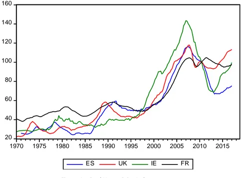
The analysis is based on quarterly data between the first quarter of 1970 and the first quarter of 2017, for three euro-area countries: Ireland (IE), Spain (ES) and France (FR), and also for the United Kingdom (UK). The reason why these countries were chosen was because the evolution of these variables in these countries was more expressive, therefore it is interesting to study the causes of this abnormal reaction. Before analyzing the results of the different approaches, it is important to analyze the evolution of the real house price index within the period of analysis (Figure 1), to see whether there are reasons to believe that there were periods of exuberant behavior (which may indicate the presence of a bubble). This index was built considering 2010 as the base year for each country.
Figure 1 shows that the evolution of the real house price index was not homogeneous over the period of analysis. Despite this, the behavior among all four countries under analysis
20 40 60 80 100 120 140 160 1970 1975 1980 1985 1990 1995 2000 2005 2010 2015 ES UK IE FR
9
was quite similar. Moreover, we can split the time range into three different subgroups: the first (subperiod I) is from the beginning of the data sample (1970) to 1996; then second (subperiod II) is from 1996 to 2008; and finally, the third (subperiod III) is from 2008 to the end of the sample (2017).
Regarding subperiod I, the price evolution is characterized by a stabilization, with a few disruptive periods of growth, namely in the UK and Spain at the end of the 80’s, which may be associated with the entrance of the “Baby Boom generation” in the real estate market. However, the growing rates end-to-end of this period were not too high for any of these countries, being Spain the country with the highest growth rate (93%), and France with the lowest (28%). Subperiod II is notable for a remarkable growth of the real house price index, in all four countries considered. Ireland was the country in which the real house price index increased the most, from a 60 in 1996 to more than 150 in 2008, i.e, a growth rate of 198%. Finally, subperiod III includes the subprime crises in the US, which brought terrible consequences for the rest of the world, especially Europe. After 2008, there was a change in paradigm, marked by a sudden decrease in the real house price index across all four countries under analysis. In this subperiod, Ireland was again the country where this change was most marked: a decrease from almost 150 in 2008 to 70 in 2012, i.e., it dropped to less than half only in just four years. France was the country where this change was not so marked. Another important issue about this period is that the index in these four countries did not behave homogeneously.
As mentioned earlier, another important indicator of the real estate dynamics is the price-to-rent ratio (Figure 2). Poterba (1984) defined this ratio as the long-run relationship between the cost of owning a property (its price) and the return in renting it out, thus this can be seen as the price-to-earnings ratio (PER) if we compare a property with a financial asset. The intuition behind this ratio is that when the cost of owning a house (its price) is too high, potential buyers find it more advantageous to rent than to buy. Intuitively, this will make the
10
demand for houses decrease, therefore the real property price will decrease, causing the price-to-rent ratio to decrease to its equilibrium value. We can do the same reasoning when the property price is too low, and the buyers find it more advantageous to buy rather than to rent. Thus, it is expected that this ratio never decreases or increase for a long period of time, otherwise, we are in an abnormal scenario. Observing the evolution of the price-to-rent ratio for the four countries under analysis, we conclude that this evolution was not constant over the period of analysis. Similarly, as observed for the real house price index, this ratio suffered the biggest change between 1996 and 2008, especially in Ireland. It can be argued that this increase in the price-to-rent ratio may be caused by unrealistic expectations about future property prices, which can lead to speculative bubbles. Also, the other three countries experimented, during this period, an abnormal increase in the cost of owning a property compared to the return of renting it out. 20 40 60 80 100 120 140 160 1970 1975 1980 1985 1990 1995 2000 2005 2010 2015 ptrES ptrUK ptrIE ptrFR
11
4. Methods and Model
The most known models used in this time-series framework are linear models, such as moving average and autoregressive models. The main advantages of linear models are their simplicity of estimation and the estimators’ properties, which make these models popular in this sort of studies. However, one can argue that the relationship between this two is not linear, that is, it may not be constant over time. In fact, as was seen in the last section, the evolution of some countries’ real house price index seems not to be constant, with periods of abnormal increases or decreases, which may not be aligned with the evolution of their determinants. Thus, it may make sense to use nonlinear models to study whether the impact of such macroeconomic determinants change in different scenarios, or not. With this in mind, both model types (linear and nonlinear) will be considered to model the impact of the different variables.
Regarding the linear model, it is important to choose a regression which allows us to study the whole distribution, instead of only the conditional mean, such as with ordinary least squares (OLS). Thus, the approach of analysis considered consists in the application of quantile regression (QR) methods. According to Machado and Sousa (2006), the benefit of using such a regression model is that the evolution of the tails of the distribution allows us to detect periods of misalignment of the real property prices with regards to its macroeconomic determinants. In other words, an interesting interpretation of the high and low quantiles is that they mark the thresholds from which the property prices are indicating the presence of a speculative bubble, or a bubble burst, respectively. Machado and Sousa (2006) made a very intuitive interpretation, using an explanatory graphic, for stock prices (see Appendix A). As can be seen, under the scenario of y0, the stock price p1 is “excessively high” and p2 is within “normal”. Although, when y0 changes to y1, p1 becomes “normal” and p2 “excessively low”. Another advantage of QR over OLS is that the former does not make any assumptions about the error term, which
12
confers an extra flexibility for modeling data with heterogeneous conditional distributions (Koenker and Hallock, 2001).
For making this analysis, it is important to choose the macroeconomic determinants that mostly impact on the long-term evolution of the real house price index. The findings in the literature indicate that these determinants could be income, construction costs, population, taxes, labor force and the return of alternative assets. However, and due to the sample length, to keep the model manageable and because to study price misalignment it is preferable to work with variables in levels instead of growth rates, only per capita disposable income, the short-term interest rate and the unemployment rate have been chosen as the deshort-terminants of the real house price index. Hence, the QR model used is the following:
rppt(𝜏|ℱ𝑡−1) = 𝛽0(𝜏) + 𝛽1(𝜏)𝑦𝑑𝑟𝑐𝑡+ 𝛽2(𝜏)𝑚𝑡𝑔𝑟𝑡+ 𝛽3𝑢𝑛𝑡+ 𝑢𝑡
where 𝜏 𝜖 (0,1) is the quantile of interest, 𝑟𝑝𝑝𝑡 represents the natural logarithm of the real house price index in period t, 𝑦𝑑𝑟𝑐𝑡 corresponds to the natural logarithm of the per capita disposable income in period t, 𝑚𝑡𝑔𝑟𝑡 is the real mortgage rate in period t and 𝑢𝑛𝑡 represents the unemployment rate in period t.
Regarding the nonlinear model, a Markov switching model (MSM) will be used. This model seems to be suitable for this analysis since the real house price index seems to have a nonlinear behavior: it fluctuates around high prices during a bubble episode, and low prices during non-bubble periods.
In the economic literature, there are several studies using this methodology, for example, Hamilton (1989) used this method to study the asymmetric behavior over GDP expansions and recessions. Also, Engel and Hamilton (1990) used a MSM to study the evolution of exchange
13
Equation 2 – Transition probability equation
Equation 3 – Transition probability matrix with k states
rates over time. However, this methodology was not only used in economics, Hamaker et al (2010) applied it to psychology, studying different manic-depressive states.
The MSM enables the time-series to transit over a set of finite states. These states are unobservable, and the transition follows a Markov process, which can switch among states throughout the sample. The time of transition between states and the duration in each state are both random. We assume that the states are defined by a random variable 𝑆𝑡 which takes the integer values 1, 2, …, N. This random variable follows a first order Markov chain, meaning that the probability of the current state only depends on the previous period's state, allowing for quick adjustments after a change of state:
𝑃(𝑆𝑡= 𝑗|𝑆𝑡−1= 𝑖, 𝑆𝑡−2 = 𝑙, 𝑆𝑡−3= 𝑘, … ) = 𝑃(𝑆𝑡 = 𝑗|𝑆𝑡−1= 𝑖) = 𝑝𝑖𝑗
where 𝑝𝑖𝑗 is the probability of the current state being j, knowing that the process was in state i
in the previous period. This means that in this process it does not matter whether a change in the current state occurred or not. We will also be interested in obtaining the expected duration of each state and the transition probability matrix, which captures the dynamics underlying this process:
[
𝑝11 ⋯ 𝑝1𝑘
⋮ ⋱ ⋮
14
Equation 4 – Markov-Switching Regression Model
Another important feature of this method is that the MSM does not require a specific threshold to change the state of the process, since the definition of each state is determined by the data. In this dissertation, we will be interested in the following regression:
𝑅𝑝𝑝𝑡 = {
𝛼1+ 𝛼2ydrct+ 𝛼3𝑟𝑒𝑛𝑡𝑡+ 𝑢𝑡, 𝑠𝑡 = 1
𝛼4+ 𝛼5ydrct+ 𝛼6𝑟𝑒𝑛𝑡𝑡+ 𝑣𝑡, 𝑠𝑡 = 2
where 𝑅𝑝𝑝𝑡 and 𝑦𝑑𝑟𝑐𝑡 have the same meaning as previously indicated, and 𝑟𝑒𝑛𝑡𝑡 corresponds to the natural logarithm of the real rent index in period t. Given that we only assume two states (with and without exuberant behavior in the real house price index), the transition probability matrix is a 2x2 matrix, comprising four probabilities.
The main motivation for the use of this methodology is to verify whether the intercept and the slope coefficients are statistically different in both states, and to draw conclusions about it. According to Nneiji et al. (2013) a rational bubble differs from an intrinsic bubble since the former appears when agents’ expectation about the future house price has an abnormal importance in the current evaluation of the price, whereas the second appears when there is an overreaction regarding changes in fundamentals. Therefore, one can argue that if 𝛼1 ≠ 𝛼4 we are in the presence of a rational bubble, and if the determinants’ coefficients differ in both states there are reasons to believe that there is an intrinsic bubble.
15
5. Results
This section analyses the estimation results of the QR and the MSM. First, it is important to mention that, although the real house price index starts in 1970Q1, some variables only start a few years later, for example, for Ireland this analysis begins in 1990Q1 because unemployment and disposable income data only start in that period.
5.1. Quantile Regression Results
Regarding QR there are mainly two interpretations to make: first of the coefficients' estimates of the lower, median and upper quantiles; and then apply the same intuition as in Machado and Sousa (2006) to assess in which periods the real house price index was misaligned with its macroeconomic determinants.
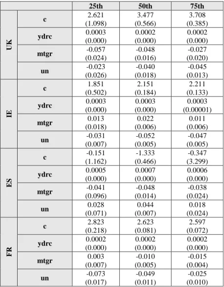
Figure 3 presents the estimates for the coefficients of the 25th, 50th (median) and 75th quantiles for the four countries under analysis. As can be seen, the real per capita disposable income (ydrc) has a similar effect in the three quantiles in all countries, and it is statistically significant at every quantile. This effect is positive, which is intuitive because when real disposable income increases, the purchasing power in the economy increases and the agents are willing to invest more in real estate, which affects prices positively. The effect of the real mortgage rate is not that similar across countries and quantiles: in the UK and Spain it has a negative effect, in Ireland it has a positive effect, and in France it has a positive effect in the lower quantile but a negative in the median and upper quantiles. It was expected that the real mortgage rate influences negatively the real house price index, because when this rate increases, the cost of owning a house will increase as well, which makes the demand for properties decrease, therefore prices also fall. Regarding the unemployment rate, the effect is heterogeneous across countries: in the UK, Ireland and France it is negative, but in Spain it is positive (it is statistically insignificant for the lower and upper quantiles). Theoretically, it
16
would be expected that an increase in the unemployment rate drives the property price down. However, as is known, sometimes a rise in the unemployment rate comes along with an increase of capital concentration, which can make prices go up.
25th 50th 75th UK c 2.621 (1.098) 3.477 (0.566) 3.708 (0.385) ydrc 0.0003 (0.000) 0.0002 (0.000) 0.0002 (0.000) mtgr -0.057 (0.024) -0.048 (0.016) -0.027 (0.020) un -0.023 (0.026) -0.040 (0.018) -0.045 (0.013) IE c 1.851 (0.502) 2.151 (0.184) 2.211 (0.133) ydrc 0.0003 (0.000) 0.0003 (0.000) 0.0003 (0.00001) mtgr 0.013 (0.018) 0.022 (0.006) 0.011 (0.006) un -0.031 (0.007) -0.052 (0.005) -0.047 (0.005) ES c -0.151 (1.162) -1.333 (0.466) -0.347 (3.299) ydrc 0.0005 (0.000) 0.0007 (0.000) 0.0006 (0.000) mtgr -0.041 (0.096) -0.048 (0.014) -0.038 (0.024) un 0.028 (0.071) 0.044 (0.007) 0.018 (0.024) FR c 2.823 (0.218) 2.623 (0.081) 2.597 (0.072) ydrc 0.0002 (0.000) 0.0002 (0.000) 0.0002 (0.000) mtgr 0.003 (0.007) -0.010 (0.005) -0.015 (0.004) un -0.073 (0.017) -0.049 (0.011) -0.025 (0.010)
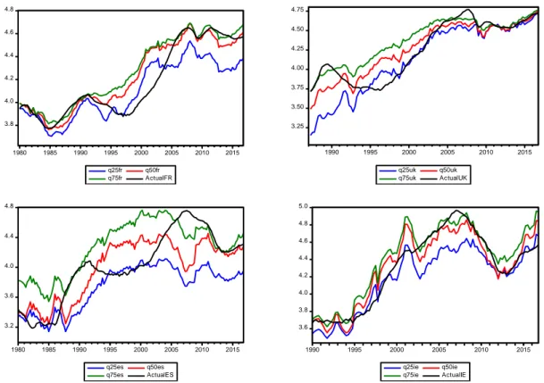
Using the fitted values of the QR, one can make an analysis similar to the one in Machado and Sousa (2006) for asset prices, i.e., track the periods of time when the property price was misaligned with its fundamental value, whether it is above (when the actual real property price is higher or near the upper quantile), or below (when it is lower or near the lower quantile). Figure 4 plots the fitted values of the QR and the actual value for the natural logarithm of the real house price index, in the four countries. As can be seen, the evolution of the quantiles
17
was not homogeneous over time, observing periods of dispersion, and the evolution of the real house price index was not always in line with the one for the quantiles, with periods where the actual real house price index increases and the fitted values for the QR are decreasing, and vice-versa. Furthermore, there is a notable similar behavior across the four countries in some time ranges. Focusing, for instance, on the last years of the 80’s, one notes that in France, the UK and Spain there is an over-valuation of the property price compared to their determinants. In Ireland, this effect appeared a few years later, and with less persistence. At the end of the last millennium, there was an opposite effect: the real house price index was under-valuated, especially in France where this effect was more intense and persistent. The last price misalignment according to this regression, occurred in the period between 2006 and 2010, especially in the UK, Spain and Ireland, where the discrepancy of the real house price index is noticeable in the upper quantile. In France, this effect was not so intense, where the real house price index was in line with the 75th quantile.
Figure 4 – Quantile Fitted Value and the actual Real Property Price
3.25 3.50 3.75 4.00 4.25 4.50 4.75 1990 1995 2000 2005 2010 2015 q25uk q50uk q75uk ActualUK 3.8 4.0 4.2 4.4 4.6 4.8 1980 1985 1990 1995 2000 2005 2010 2015 q25fr q50fr q75fr ActualFR 3.2 3.6 4.0 4.4 4.8 1980 1985 1990 1995 2000 2005 2010 2015 q25es q50es q75es ActualES 3.6 3.8 4.0 4.2 4.4 4.6 4.8 5.0 1990 1995 2000 2005 2010 2015 q25ie q50ie q75ie ActualIE
18 5.2. Markov-Switching Model Results
The results of the MSM may be more interesting since it assumes a nonlinear relationship between the real house price index and its determinants, but it also allows us to split the sample into two regimes and allocate each observation to a specific regime endogenously, which is a very important feature to study the real estate dynamics, especially in periods with price misalignment. Firstly, and before starting to analyze the coefficient estimates from this model, it is important to state which periods of each country the model assumes as a period of misalignment of price, or not, which is given by the predicted regime probabilities. After analyzing these probabilities and the coefficient estimates, it is necessary interpret the constant expected duration of each regime, and the regime transition probability matrix as well. It should be noted that although the results of the four countries will be commented, the outputs presented will be only for Spain, however the results of the remain countries can be found in the appendix.
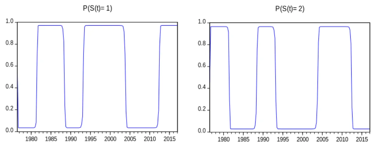
Figure 5 shows the MSM predicted regime probabilities for Spain, which allows one to establish the correspondence between each regime, where the left graph represents the probability of each period to be in regime 1, and the right graph the probability of each period to be in regime 2.
Figure 5 – Markov Switching Predicted Regime Probabilities for Spain
0.0 0.2 0.4 0.6 0.8 1.0 1980 1985 1990 1995 2000 2005 2010 2015 P(S(t)= 1) 0.0 0.2 0.4 0.6 0.8 1.0 1980 1985 1990 1995 2000 2005 2010 2015 P(S(t)= 2)
Markov Switching One-step Ahead Predicted Regime Probabilities
0.0 0.2 0.4 0.6 0.8 1.0 1980 1985 1990 1995 2000 2005 2010 2015 P(S(t)= 1) 0.0 0.2 0.4 0.6 0.8 1.0 1980 1985 1990 1995 2000 2005 2010 2015 P(S(t)= 2)
19
Hence, for Spain (Figure 5), we observe three periods during which clearly regime two prevails: the first is from the begin of the sample until 1981; the second is from 1988 to 1994; and the third is between 2003 and 2012. As we saw in the section on “Data description”, these were the periods in which abnormal behavior in the evolution of the real house price index predominated. The remaining periods were allocated to regime one, where there is an apparently normal behavior in the evolution of the property prices. Regarding the other countries, the most identical to Spain is the one from the United Kingdom where regime two comes up first in the nearly 90’s and then from 2003 onwards. In Ireland it is quite distinct, since the only time range where regime two appears is between 2002 and 2009. France has a slightly different behavior as regime two has a longer duration.
The analysis of the coefficient estimates is truly essential in order to see whether the abnormal behavior of the property price comes from an overreaction of changes in the fundamentals, which can be detected if the estimates of one or more variables is statistically different in both regimes; or whether this abnormal behavior is due to an unrealistic expectation about the future evaluation of the property. This last point is detected if one can see any statistically difference in the intercept of the models.
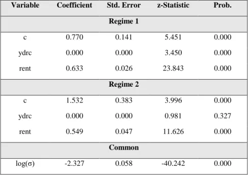
Variable Coefficient Std. Error z-Statistic Prob.
Regime 1 c 0.770 0.141 5.451 0.000 ydrc 0.000 0.000 3.450 0.000 rent 0.633 0.026 23.843 0.000 Regime 2 c 1.532 0.383 3.996 0.000 ydrc 0.000 0.000 0.981 0.327 rent 0.549 0.047 11.626 0.000 Common log(σ) -2.327 0.058 -40.242 0.000
20
Figure 6 presents the estimation output of the MSM for Spain. To draw conclusions about the differences under both regimes in the value of the coefficients, we must compute a Wald test, with the following null hypothesis (note that the coefficients used in this hypothesis are the same as in equation 4):
𝐻𝑜: 𝛼1 = 𝛼4⇔ 𝛼1− 𝛼4 = 0
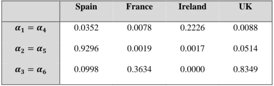
This specific null hypothesis is for the intercept, but one also needs to compute a similar test for the other two coefficients (disposable income and rent). The criteria used to reject the null hypothesis is the value of the t-test, with the significance level of 5%: whenever the p-value is smaller than 0.05, we have statistical evidence to reject the null hypothesis. Figure 7 exposes the p-values for the null hypothesis across the four countries.
For instance, for Spain, one can conclude that there is evidence to reject the null hypothesis that the intercept is equal under both regimes, since its p-value is 0.0352. But, the p-value for the disposable income is 0.9296 and for rent it is 0.0998. Thus, we can state that for Spain, what it is behind the change of regime is the change in the intercept. The UK is similar to Spain, since only the intercept’s coefficient changes in both regimes (p-value=0.0088). For France, the effect of disposable income is also different in each regime (p-value=0.0019), as well as the intercept (p-value=0.0078). In Ireland the intercept does not change with the regime (p-value=0.2226). However, the other two coefficients vary over the regimes with a p-value of 0.0017 for disposable income and a p-value of 0.000 for rent.
Spain France Ireland UK
𝜶𝟏= 𝜶𝟒 0.0352 0.0078 0.2226 0.0088
𝜶𝟐= 𝜶𝟓 0.9296 0.0019 0.0017 0.0514
𝜶𝟑= 𝜶𝟔 0.0998 0.3634 0.0000 0.8349
Equation 5 – Wald-Test null hypothesis
21
Finally, other important indicators are the transition probability matrix and the constant expected duration of each regime. These two estimates give us a more robust information about the persistence of each regime. Starting with the transition probability matrix, one obtains the following matrix for Spain:
[
0.95 0.05
0.04 0.96
]
As mentioned in the previous section, 𝑝𝑖𝑗 corresponds to the probability of changing the regime, when the previous period regime was i and the current regime is j. Thus, we can see that the persistence of both regimes is quite large, since the probability of the last quarter’s regime prevailing in the current quarter is in every case higher than 95%, for Spain and for the other countries as well.
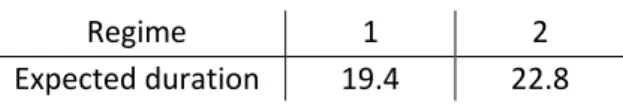
The constant expected duration for Spain is:
Regime 1 2
Expected duration 19.4 22.8
For Spain, the expected duration of regime two (22,8 quarters) was higher than the one of regime one (19,4). In the other countries, the opposite is verified: regime one lasts longer than regime two. Refer to appendices C and D for detailed information about the transition probability matrix and constant expected duration for France, Ireland and the United Kingdom.
Equation 6 – Transition Probability Matrix for Spain
22
6. Conclusion
The present dissertation analyzed the dynamics of the real house price index for four European countries (Spain, France, United Kingdom and Ireland) between 1970 and 2017, with the following objective: to determine whether there is statistical evidence of a bubble in the European real estate market over the recent years or not; and then, if so, determine whether these were intrinsic or rational, according to the definition proposed by Nneiji et al. (2013). Whereas a linear model is sufficient to achieve the first goal, the second one requires a nonlinear model.
First, a preliminary analysis was made of the evolution of the real house price index from 1970 to 2017, in order to determine the periods during which the price evolution raised doubts. Also, the most-known valuation ratio – price-to-rent – was analyzed to determine during which periods the price was not in line with its rate of return (rent). In both analyses, the periods from 1985 to 1990 and from 2000 and 2008 suggest an abnormal evolution. However, one cannot tell at this point that this is a bubble because the deviations from its fundamental value were not analyzed. Thus, a quantile regression was applied with the aim to determine the periods where this deviation was verified. In this model the real per capita disposable income, the mortgage rate and the unemployment rate were used as the macroeconomic determinants. The model points to the periods previously referred as the periods during which the real house price index exceed the upper quantile, therefore periods where there is statistical evidence to state that there was a considerable price deviation from their fundamental value.
Lastly, a Markov-Switching Model was computed with the goal to understand whether the deviations from the fundamental value is due to an overreaction to some determinant, or if it is caused by an unrealistic expectation about future appreciations of the properties. For this application the per capita disposable income and rent were used as explanatory variables. The main conclusions of this model are that the bubble type varies a lot across the four countries
23
analyzed. Whereas the deviations of Spain and the UK were due to differences in the intercept (rational speculative bubble), in Ireland it was due to an overreaction in some periods to changes in disposable income and in the price of rents. In France, it seems to be a combination of both: it was shown that there was an overreaction to changes in disposable income and a change in the intercept of the model.
Regarding the weaknesses and limitations that were felt in this research, they are related to the fact that there is a lack of data for Ireland and the UK, namely for the mortgage rate and the unemployment rate. In addition to limiting the period of analysis, this drawback leads to a decrease in the flexibility of the Markov switching model to incorporate more variable into the analysis, failing to produce feasible outputs when one increments the number of fundamental variables of the model.
I hope that the acknowledgment of this limitations may trigger some improvements to the research in this framework, which can be through the extension of this study to more countries, not only the European ones, that could bring new insights into how culture might affect the house prices misalignment. Using a more extended number of observations of each variable might improve the flexibility and reliability of the Markov-switching model, as well.
24
7. References
Agnello, L. and L. Schuknecht. 2009. “Booms and Busts in Housing Market”. European Central Bank, Working Papers Series No. 1071
Ardila, D., D. Sanadgol, P. Cauwels and D. Sornette. 2014. “Identification and Critical Time Forecasting of Real Estate Bubbles in the U.S.A. and Switzerland.” ETH Zurich. Case, K.E., J.M. Quigley and R.J. Shiller. 2005. “Comparing Wealth Effects: The Stock Market
versus The Housing Market.” Advances in Macroeconomics 5(1). Article 1
Chakraborty, S. 2009. “Economic Fundamentals, Real Estate Dynamics and Business Cycles in Japan.” Baruch College.
Chen, R., C. Gan, B. Hu and D.A. Cohen. 2013. “An Empirical Analysis of House Price Buble: A Case Study of Beijing Housing Market.” Macrothink Institute, Research in Applied Economics.
Detken, C., and F. Smets. 2004. “Asset Price Booms and Monetary Policy.” European Central Bank, Working Papers 0364.
Fama, E. 1970. “Efficient Capital Markets: a Review Of Theory and Empirical Work.” Journal of Finance 96, 246-273.
Gallin, J. 2004. “The Long-Run Relationship Between House Prices and Rents.” Federal Reserve Board.
Gelain, P., and K.J. Lansing. 2014. “House Prices, Expectations, and Time-Varying Fundamentals.” Federal Reserve Bank of San Francisco. Working Papers Series. Ghysels, E., A. Plazzi, W. Torous and R. Valkanov. 2012. “Forecasting Real Estate Prices.” Glaeser, E.L. and C.G. Nathanson. 2015. “An Extrapolative Model of House Price Dynamics.”
Harvard Kennedy School. Faculty Research Working Paper Series.
Granziera, E., and S. Kozicki. 2012. “House Price Dynamics: Fundamentals and Expectations”. Bank of Canada. Working Paper 2012-12.
Hamilton, J.D. 1989. “A New Approach to the Economic Analysis of Nonstationary Time Series and the Business Cycle.” Econometrica, Vol.57 No 2, 357-384.
Kahn, J.A. 2008. “What Drives Housing Prices?” Federal Reserve Bank of New York, Staff Reports No. 345.
25
Kemme, D.M. and R. Saktinil. 2012. “Did the Recent Housing Boom Signal Global Financial Crisis?” Southern Economic Journal 78(3): 999-1018.
Koenker, R. and K.F. Hallock. 2001. “Quantile Regression”. Journal of Economics Perspectives 15(4): 143-156.
Loureço, R. and P. Rodrigues. 2015. “House Prices: Bubbles, Exuberance or something else? Evidence from Euro Area Countries”. Banco de Portugal, Estudos e Documentos de Trabalho, Working Papers 17.
Lu, D. 2016. “Analysis of Real Estate Price Dynamics in Switzerland Using a Fundamental Factor Model.” Master Thesis. Swiss Federal Institute of Technology Zurich.
Machado, J. and J. Sousa. 2006. “Identifying Asset Price Booms and Busts with Quantile Regressions”. Banco de Portugal, Estudos e Documentos de Trabalho, Working Papers 8.
Mankiw, N.G. and D.N. Weil. 1989. “The Baby Boom, the Baby Bust, and the Housing Market.” Harvard University
Nneiji, O., C. Brooks and C. Ward. 2013. “Intrinsic and Rational Speculative Bubbles in the U.S. Housing Market: 1960-2011.”
Paliouras, D. 2007. “Comparing Regime-Switching Models in Time Series: Logistic Mixtures vs. Markov Switching.” Master Thesis. University of Maryland.
Poterba, J. 1984. “Tax Subsidies to Owner-Occupied Housing: An Asset Market Approach.” Quarterly Journal of Economics 99(4):729-752.
Shiller, R.J. 2008. “The Subprime Solution: How Today’s Global Financial Crisis Happened, and What to Do about it.” Princeton University Press.
Zhou, J. 2010. “Testing for Cointegration Between House Prices and Economic Fundamentals.” Real Estate Economics 38(4): 599-632.