Forecasting large covariance matrices: comparing autometrics and LASSOVAR

(1)

Forecasting Large Covariance Matrices: Comparing

Autometrics and LASSOVAR

Ronan Cunha

∗

Anders Bredahl Kock

†

Pedro L. Valls Pereira

‡

Abstract

This study aims to compare the performance of two well known automatic model selection algorithms, Autometrics (Hendry and Krolzig, 1999; Doornik, 2009), LASSOVAR and adaptive LASSOVAR (Callot et al., 2017) for modelling and forecasting monthly covariance matrices. To do so, we compose a database with daily information for 30 Brazilian stocks, which yields 465 unique entries, from July/2009 to December/2017. We apply three forecasting error measures, the model confidence set (Hansen et al., 2011) and Giacomini and White (2006) conditional test in the comparison. We also calculate the economic value for each of the forecasting strategy through a portfolio selection exercise. The results show that the individual models are not able to beat the benchmark, the random walk, but a weighted combination of them is able to increase precision up to 13%. The portfolio selection exercises find that there are economic gains for using automatic model selection techniques to model and forecast the covariance matrices. Specifically, under short-selling constraint, Autometrics VAR(1) with dummy saturation delivers the highest Sharpe-ratio and economic value. When the investor is able to short-sell, either Autometrics VAR(1) with dummy saturation or adaptive Lasso VAR(1) is preferable. This final choice depend on the risk aversion of the investor. If he is less risk-averse, he prefers the former, while the latter becomes his choice if his risk-aversion sensitivity increases.

Key words: Forecasting, Covariance Matrix, Autometrics, Lasso, Vector Autoregression, Portfolio Allocation, Economic Value.

JEL Code: C32, C53, C58, G11.

∗_{Sao Paulo School of Economics - FGV and CEQEF - FGV. This study was financed in part}

by the Coordena¸c˜ao de Aperfei¸coamento de Pessoal de N´ıvel Superior - Brasil (CAPES) - Finance Code 001”. E-mail: cunha.ronan@gmail.com

†_{Oxford University, Aarhus University and CREATES, Department of Economics, Manor Road,}

Oxford, OX1 3UQ, UK. E-mail: anders.kock@economics.ox.ac.uk.

‡_{Sao Paulo School of Economics - FGV and CEQEF - FGV. E-mail: pedro.valls@fgv.br. The}

third author acknowledges financial support from CNPq (309158/2016-8) and FAPESP (2013/22930-0.).

(2)

2

( (

2 2

1 Introduction

Forecasting and modelling covariance matrices have attracted the interest of researchers and financist due to its great importance in portfolio selection, risk management and hedging strategies (Engle, 2009; Hlouskova et al., 2009; Boudt et al., 2013, for instance). Indeed, the classical mean-variance approach of Markowitz (1952) relies on estimating all the entries of this matrix which may become a big challenge, especially when the number of assets grows. Standard methods, such as, Baba-Engle-Kraft-Kroner (Baba et al., 1990; Engle and Kroner, 1995, BEKK) and dynamic conditional correlation (Engle, 2002, DCC) fail to deliver reliable estimates due to the curse of dimensionality (Callot et al., 2017).

Dimensionality is a serious challenge for the traditional forecasting models in this literature. The number of distinct entries grows exponentially with the number of assets. In a setup with n assets, there are n(n + 1)/2 distinct entries in the covariance matrix. Furthermore, if we model them as a vector autoregressive of order p, VAR(p), there are n(n+1) n(n+1) p + 1 parameters to estimate, including

the intercepts. For instance, it means that for only 30 assets in a VAR(5), which is used in this paper, there are 465 equations and 1,081,590 parameters.

Besides the advances in estimation methodologies, such as, random matrix theory, new methods are also developed to easily construct dynamic models to the covariance matrix based on shrinkage procedures (Callot et al., 2017; Brito et al., 2018).

In this paper, we follow Callot et al. (2017) and we use the advances in model selection methodologies to deal with the curse of dimensionality aiming to accurately model and forecast all entries of the covariance matrix. Instead of using the Lasso approach as the authors, we apply the general to specific approach, Autometrics. The latter has useful improvements over other algorithms. For example, Autometrics takes the behavior of the residuals into consideration in the selection and it can easily identify structural breaks and outliers through impulse indicator saturation and its extensions (Ericsson, 2012). Outliers can seriously damage the estimation of the covariance matrix (Truc´ıos, Hotta, and Pereira, Truc´ıos et al.; Hotta and Truc´ıos, 2018) and its economic application (Truc´ıos et al., 2018).

Therefore, the main objective of this paper is to compare the forecasting performance of Autometrics and LASSOVAR when handling high dimensional system of equations. To do so, we use three different error forecasting measures as in Callot et al. (2017) and also the model confidence set (Hansen et al., 2011) and Giacomini and White (2006)’s conditional predictive ability test. We analyze the usefulness of those methods when forming investment portfolios under different environments as in Brito et al. (2018) and Callot et al. (2017). We also discuss the drivers of the dynamic of the covariance matrices over time and how they change between those methods.

The database composes daily information for 30 Brazilian stocks traded in Bovespa stock market (B3) from 2009 till 2017. Due to the promising performance found in Callot et al. (2017), we also model the logarithm of the covariance matrix (Chiu et al., 1996). Due to the lack of high frequency data for longer periods, daily data is applied to estimate the monthly covariance matrix.

(3)

The results show that it is not easy for individual models to beat the benchmark which is a random walk, but a weighted combination of them is able to increase precision up to 13%. The model confidence set show that those two methods are in all final sets and, most of the time, ranked either as first or second depending on the forecasting horizon and error measure. Giacomini and White (2006) conditional test confirms that both methods delivers equal forecasts to all forecasting horizons and error measures.

The portfolio allocation exercises show that there are economic gains replacing the no-change forecast to one of the alternative forecasting strategies, specially when short-selling is a constraint. Out of all methods, Autometrics VAR(1) with dummy saturation returns the best investment performance without short-selling measured as accumulated return. This strategy also delivers very competitive Sharpe-ratio. When shortselling is permitted, the preferable strategy depends on the investor’s risk-aversion. For less risk-averse investors, Autometrics VAR(1) with dummy saturation has higher economic value. For more risk-averse investors, adaptive LASSO- VAR(1) returns the best value though not the highest accumulated return. However, for more highly risk-averse investors, adaptive LASSOVAR(1) is preferable if short- selling is not a restriction.

The paper is organized as following. Next section, we present the literature review and describe the two automatic selection methods compared in this study. The third section, we present the methodology and comparison strategy. In the first part of the forth section, we describe the selected models and their drivers. In the second part of this section, we present the forecasting error measures and the model confidence set results. The fifth section, there the portfolio management exercise and, the last section concludes this study.

2 Literature review

2.1 Forecasting Large Realized Covariance Matrix

Estimating, modelling and forecasting covariance matrices have been heavily studied in economics due to its substantial importance for risk management and asset allocation. In practice, the true covariance matrix is not directly observable. The traditional strategies to estimate it is to apply multivariate GARCH (Bollerslev et al., 1988) and its extensions, e.g. BEKK (Baba et al., 1990; Engle and Kroner, 1995), CCC (Bollerslev, 1990) and DCC (Engle, 2002) models. However, these models impose strong restrictions on the parameters to be estimated and they heavily depends on the underlying process of the covariance matrix (Bucci, 2018). Further- more, another caveat is that they also suffer from the curse of dimensionality failing to deliver reliable estimates if the number of assets in consideration is large1 (Callot et al., 2017).

The evolution of financial markets, has not only increased the number of assets available and also has worsened the curse of dimensionality problem, but also put available intra-day data. Merton (1980) had already showed that volatility can be

(4)

4

( (

2 2

defined as the sum of the squared returns at high frequency level. Andersen et al. (2001) pointed out that an observable measure of daily volatility can be obtained by summing up the squared intra-daily returns. Later, Andersen et al. (2003) showed that using the same approach it is possible to obtain all daily co-volatilities between assets, named realized covariance matrix.

The use of realized covariance has been very beneficial for investment decisions. (Fleming et al., 2003) calculated that a risk-averse investor would be willing to pay 50 to 200 basis point per year to switch from daily to intra-daily returns in order to estimate the covariance matrix.

Nevertheless, the curse of dimensionality has still been a concern. As pointed out by Bai et al. (2011) sample covariance matrix may have some undesirable properties when its dimension is large. First, when the number of asset is larger than the number of observation, the matrix is not full rank, thus it is not invertible. Second, even when it is, the expected value of its inverse is a biased estimator to its theoretical inverse. Third, the sample covariance may be very volatile and it may induce high weights turnover in the portfolio and it tends exceed the targeted risk out of sample. Some papers have dealt with this issue, for instance, Barndorff-Nielsen and Shephard (2004), Bickel et al. (2008), Hautsch et al. (2012), Fan et al. (2013), Lunde et al. (2016) and, for a literature review about large covariance estimation methodologies, Bai et al. (2011) and Fan et al. (2016).

When the objective turns from the estimation of the integrated covariance matrix to modelling its dynamics in order mainly to increase forecasting power, the curse of dimensionality is an issue to overcome. As highlighted previously, tra- ditional models also suffer from the curse of dimensionality. In a set up with n assets, there are n(n + 1)/2 distinct entries in the covariance matrix. Further- more, if we model them as a vector autoregressive of order p, VAR(p), there are

n(n+1) n(n+1)

p + 1 parameters to estimate, including the intercepts. For in-

stance, if an investor considers a set of 30 assets to allocate in its portfolio and he models each distinct entry of the covariance matrix as a VAR(1), it means a system of 465 equations with 495 parameters to be estimated. If, instead, he uses a VAR(10), there are 2,162,715 parameters.

There are some recent papers in the realized covariance matrix forecasting literature dealing with the dimensionality problem. Bauer and Vorkink (2011) adapted the heterogeneous autoregressive (HAR) model (Corsi, 2009) to multivariate context. In order to reduce the number of parameters to be estimated, they apply principal components. They showed that a few latent factors are able to explain the dynamics of the covariance matrix. They calculated the co-volatilities using Barndorff-Nielsen and Shephard (2004)’s estimator and use logarithmic covariance (log Cov) of Chiu et al. (1996) to ensure positive definiteness. Chiriac and Voev (2011) developed a vector autorregressive fractionally integrated moving average (VARFIMA) model. As opposite to Bauer and Vorkink (2011), the apply Cholesky decomposition to ensure positive definiteness matrix. Their procedures if based on three steps: i) the covariance matrix is decomposed into Cholesky factors; ii) these factors are modelled and predicted using VARFIMA model and; iii) the covariance matrix is recomposed with the forecast factors. Gouri´eroux et al. (2009) and its extension by Golosnoy et al. (2012) proposed the use autorregressive Wishart model

(5)

×

to capture the dynamic of covariance matrix. The common drawback of all those studies is they still suffer from the curse of dimensionality when the number of assets grows (Callot et al., 2017). Indeed, Golosnoy et al. (2012) pointed out that their model may be applicable to about ten assets. They also used a few assets from North America’ stock market2

in their empirical exercise.

In this contexts, there are a few recent sutdies focusing on more flexible ap- proaches to tackle the high dimensionality problem. Callot et al. (2017) modelled the dynamic of the n n realized covariance matrix (Σt) as a vector autoregression of order p. In the paper p is equal to 1, 5 and 20. Each distinct entry of the matrix is an equation which is composed of the p lags of all the other entries. Thus, the whole system has k = n(n + 1)/2 equations and k (kp + 1) parameters to estimate. The authors constructed the upper bound of the covariance matrix forecasting error and how it translates to the portfolio variance forecasting error for Lasso and adaptive Lasso. They also apply the methodology to 30 assets from USA for daily, weekly and monthly aggregations. To ensure positive definiteness, they apply two strategies: i) logarithmic covariance matrix (log Cov) as in Chiu et al. (1996) and, ii) eigenvalue cleaning as in Hautsch et al. (2012). Their results show that it is not easy to beat the benchmark of no change but the log Cov outperformed all the other models more frequently in all aggregation levels. They also estimated that a risk-averse investor is willing to pay 11% per year to switch from the no change forecast to the log Cov model.

Engle et al. (2017) combined the composite likelihood method of Pakel et al. (2017) which allows the estimation of large dimensional DCC models with non- linear shrinkage method of Ledoit and Wolf (2017) derived from Random Matrix Theory. Using CRSP data, they constructed portfolios with up to 1000 assets and they showed their method outperforms alternative strategies, such as, traditional DCC models and Riskmetrics 2006 (Zumbach, 2007).

Another study that also dealt with a large number of assets, 430 stock from com- posing S&P500, is Brito et al. (2018). They put forward a methodology which com- bines asset pricing factor models, heterogeneous autoregressive models and Lasso. They argued that, although the previous procedures are able to deal with large number of assets, they become unfeasible if the number of assets keeps growing. Computationally speaking, the previous methods indeed have this requirement.

The recent studies rely on the shrinkage methods, especially adaptive Lasso (Tibshirani, 1996; Zou, 2006). However, there are alternative model selection methods which, in essence, could also be applied to model the covariance matrix similarly to Callot et al. (2017). In the next section, we present Autometrics which is an alternative method to Lasso and extensions.

2.2 Automatic Model Selection Methods

Automatic Model Selection methods have gained importance in econometrics due to the increasing amount of available data. Researchers need to deal with highly dimensional models that sometimes make the estimation totally infeasible. The

2_{Bauer and Vorkink (2011) and Golosnoy et al. (2012) used five and Chiriac and Voev (2011)}

(6)

6 L × × c

traditional selection methods, such as R2 and information criteria are impracticable if the number of candidate variables is large. The space of potential final models exponentially increases with the number of candidates. If there are k candidate variables, there are 2k possible final models.

In this paper, we compare the forecasting performance of two automatic model selection techniques. The first is Lasso and its extension, adaptive LASSOVAR, that we present in the next section and the second is Autometrics which belongs to a different class of section models called General to specific (Gets) approach developed by Hendry and Krolzig (1999); Doornik (2009).

2.2.1 Lasso for Vector Autoregressive model (LASSOVAR)

The least absolute shrinkage and selection operator, or as it is better known Lasso, was proposed by Tibshirani (1996). The methods is based on the maximiza- tion of the square residuals subject to the sum of the absolute regression coefficients which allows the selection and estimation of the parameters simultaneously. It has gained popularity due to its ability to shrink a coeffients to zero and return a sparse model (Zhao and Yu, 2006).

Besides these desired characteristics, Zou (2006) showed that Lasso is consistent under nontrivial conditions and it lacks the oracle property. Thus, Zou (2006) put forward the adaptive Lasso which fixs those problems. This method use adaptive weights to penalize different coefficients.

Lasso and adaptive Lasso have been developed under the context of a single equation to model the conditional mean. Callot et al. (2017) extended the methodology to system of equations to model all entries of the covariance matrix. They developed this method as an alternative and a more flexible approach to tackle the curse of dimensionality when dealing with an increasing number of assets.

Callot et al. (2017) modelled the dynamic of the n×n realized covariance matrix (Σt) as a vector autoregression of order p. Each distinct entry of the matrix is an equation which is composed of the p lags of all the other entries. Thus, the whole system has k = n(n + 1)/2 equations and k (kp + 1) parameters to estimate. We can to write the system as

p

yt = w + Φiyt−i + et, t = 1, . . . , T (1)

i=1

where yt = vech (Σt) and vech(.)3 is the half-vectorization operator return a vector of length n(n+1)/2 with the unique entries of Σt. Φi is the k k matrix of parameters of the i-th lag and w is the n(n + 1)/2 1 vector with the intercepts.

To circumvent the dimensional problem, Callot et al. (2017) show that it is possible to apply Lasso by Tibshirani (1996) and adaptive Lasso (Zou, 2006) equation by equation to select the number of relevant regressors. Thus, Φ = (Φ1, . . . , Φp) will

be a sparse matrix.

3_{Define A =} a b

a b

(7)

( × × 1 i=1 i = L ) + (β = 0) × log(T ), (4),i ij { } ∪ 2

For convenience, we shall rewrite equation (1) in a stacked form. Let Zt =

1, y_t₋₁, . . . , y_t_−pbe the kp + 1 vector of explanatory variables as time t and Z = (ZT

, . . . , Z1) the T (kp + 1) matrix of covariates for each equation. Let yi = (y_T,i, . . .

, y1,i) be the T 1 vector of observations on the ith variable (i = 1, . . . , k)

and ei = (eT,i, . . . , e1,i). Finally, γi = (wi, β_i) is the (kp + 1) parameter vector of

equation i. The stacked form of (1) is

yi = Zγi + ei, i = 1, . . . , k (2)

The main assumption for the estimation of model (2) is the sparsity of γi. Let γˆi be the estimator of γi which is the solution to the following minimisation problem4:

γˆi = argmin { \yi − Zγi\2 + 2λT \βi\/! } , (3)

γ∈Γ

where \x\ = m x2, \x\/! m _i=1|xi| and λT is the weight of the penalty term and it is selected through the Bayesian Information Criterion (BIC). Thus, the BIC for equation i and penalty parameter λT is

BICi(λT ) = T × log(eˆλT,ieˆλT

kp

ˆλ _ij

j=1

where eˆλT ,i is the vector of residuals and βˆλ are the estimated β corresponding to

penalty parameter λT .

For the adaptive Lasso, Callot et al. (2017) proposed to apply Lasso in a first stage to reduce the dimensionality and thus to use estimated parameters as the weights for adaptive Lasso, in the second stage.

Formally, let J (βî) = {j ∈ IRkp : βî,j = 0} be the indices of the coeffients considered nonzero by Lasso for equation i and J˜i(γî) = 1 J(βî) + 1 where we can understand the set addition elementwise.

Let γˆadap be the estimates coefficients by adaptive Lasso, thus γˆadap is the solution to the following minimization problem:

γâdap_{= argmin} 1 \y _{− Z} J˜(γî) γi,J˜(γî) \ + 2λT L _|β_i,j_| , i = 1, . . . , k (5) γ∈J˜(γî) T _{j∈J (βˆ} i) |βi,j |

This approach allows the application of adaptive Lasso in a setting where there are more candidate variables than observations. A drawback of this methodology is that it does not take the behavior of the residuals into consideration in the selection process. Thus, it is not guaranteed that the residuals of the final model are congruent. Autometrics, which we present in the next section, takes the behavior of the residuals into consideration by applying a set of diagnostic tests during the selection process. ˆ i i i 1 i

(8)

8

4_{Just for comparison, in Tibshirani (1996), the minimization problem is \yi}_{− Zγ}

(9)

2.2.2 Autometrics

Autometrics (Doornik, 2009) is a multi-path general to specific model selection algorithm. It is an extension of Hoover and Perez (1999) and Hendry and Krolzig (1999) which are derived from the Hendry (1995)’s theory of reduction.

It is implemented in OxMetrics 8 and it follows the following step:

1. General Unrestricted Model (GUM): The GUM is the initial model which en- compasses the whole information, that is, all candidate variables. It is equation (2). It is expected to encompass the parsimonious congruent models, otherwise, it will suffer with omitted variable bias (Castle and Hendry, 2010). 2. Dummy saturation: In order to control for structural breaks and outliers, Au-

tometrics applies Impulse Indicator Saturation (IIS), Step Indicator Saturation (SIS), Zero sum pairwise IIS (DIIS) and extensions, see Ericsson (2012). 3. Tree search: this is the main difference from the multi-path strategy in Hendry

and Krolzig (1999) algorithm. Chosen a significance level, each variable or a group of variables is deleted. To efficiently search, Autometrics maps all possible models and it structures the tree search in a way that avoids estimating the same models twice.

4. Highly correlated regressors: It is well known that highly correlated regressors are problematic for all model selection algorithms. For Autometrics, in particularly, if there is a relevant variable highly correlated with another re- gressor, it tends to exclude them due to inflation in standard errors. In order to avoid that important variables are removed because of that, Autometrics also searches for possible variables that should be re-included. It looks for models in the set of previous excluded variables.

5. Diagnostic test: The behavior of error is also assessed. In order to be considered a final candidate it must pass in the diagnostic tests pre-specified.

6. Tie-breaker: In the end of each branch of the tree search, there is a final candidate. They are merged and become the new GUM. The interaction goes on until the next GUM be equal to the previous one. If there are still more than one model that passes in the diagnostic test, the finalist may be either the union of them or selected by information criteria.

Its procedure is very intuitive as it has been designed to follow more rigorous and concisely the procedure researchers would do manually. As pointed out by (Castle et al., 2013), model selection may lead them to fall into the data-mining trap.

Autometrics can also handle system of equation as vector autoregressive models. However, in this study, we apply the selection methods equation by equation as the number of equations in our model is greater than the number of observation as it will be described in the next section.

Autometrics’ theoretical consistency and properties have been demonstrated in some papers. Campos et al. (2003) mapped information criteria into the implicit significance levels approach which is the exclusion criterion used by Autometrics to study its statistical properties. Hendry and Krolzig (2005) showed how to de- bias the estimator after repeated and sequentially hypothesis test which truncates the t-Student distribution far from the origin, consequently, generating coefficients which are upward bias and standard error which are downward biased. Johansen

(10)

10 L

1 d

average return of stock i.

i

t tτ =1 tτ i

and Nielsen (2009) showed the robustness of impulse indicator saturation and they derived its asymptotic distribution.

Epprecht et al. (2019) also studied the performance of Lasso against Automet- rics but in a different setup. While we compare those methods in system of equations for modelling covariance matrices, the authors analyzed univariate case for conditional mean. They reported, through simulation that when the number of variables is larger than the number of observations, both methods performed similarly. Us- ing real data, Autometrics presented better results in-sample measured by R2 while using a modified version of Diebold and Mariano (1995) test of predictive accuracy (Harvey et al. (1997)) Lasso, adaLasso and Autometrics are not distinguishable.

3 Methodology

3.1 Databases and construction of the covariance matrix

The database composes the daily closing prices of the 30 most liquidity stocks5 over the period 2009 and 2017. We split the database from 2009 to 2014 for the first estimation sample and we forecast from January 2015 till December 2017. We apply a rolling window of 60 observation and we forecast up to 6 months ahead.

We compute the monthly covariance matrix (Σt) using daily stock returns. Let

rtτ = ln(ptτ /ptτ−1 ) be the return of stock i in month t and day τ , where ln is the

napierian logarithm. We calculate the covariance between the i − th and j − th stocks for month t, σij,t, according to:

1 σij,t = t td (rtτ i − r¯i)(r tτ j − r¯j), (6) d tτ =1

where t is the number of days in month t and r¯ = Td

r is the monthly

In order to ensure that we forecast positive definite matrix, we model the logarithm of the variance (Chiu et al., 1996; Bauer and Vorkink, 2011). The reason for this choice is because Callot et al. (2017) found that the log covariance delivers the best performance if compared to other methods of ensuring positiveness, such as the eigenvalue cleaning (Hautsch et al., 2012).

3.2 Computing the Forecast

After selecting the variables and estimating the vector of parameters γˆi for equation i, we do the forecasts as usual in VAR models. The one step ahead forecasts are given by equation (7). The forecasts to (T + h) step is done recursively using the previous periods’ forecasts, as in equation (8).

yˆi,T+1|T = γˆ_iZ_T . (7)

(11)

11

(12)

12

{ }

yî,T +h|T = γîZˆT +h−1|T . (8) Non-linear models may produce forecasts clearly unreasonable (Swanson and White, 1995, 1997; Teräsvirta et al., 2003). To deal with it, Swanson and White (1995) came up with a filter which unrealistic forecasts are replaced by reasonable ones. They named this procedure, insanity filter. Furthermore, Kock and Teräsvirta (2014) showed that it may also improve forecasting accuracy of three automatic model selection: Autometrics, QuickNet and Marginal bridge estimator. Callot and Kock (2014) applied this filter to Lasso and adaptive Lasso.

Therefore, we also use this filter to trim insane forecasts as in Callot and Kock (2014) and Callot et al. (2017). If yˆi,T +h|T ∈/ [yT ± 4 × SD], where SD is the standard

deviation in the estimation sample, we replace yˆi,T+_h|T with y_T . We substitute

insanity for ingenuity. Kock and Ter¨asvirta (2014) noted that the particular choice of insanity filter is not important; what matters is to eliminate unrealistic forecasts. As the forecasts computed are recursively, we weed out the forecast outside the interval before forecasting the next period. The reason for this choice is that an unreasonable is most likely to generate another unreasonable forecast. Using this procedure, we reduce the number of replacements.

3.3 Forecasting combination

Many studies advocates that there are gains in precision when combining forecast from different models (Granger, 1969; Granger and Ramanathan, 1984), we also test its performance for the covariance matrix. Cavaleri and Ribeiro (2011) show the improvement for Brazilian volatility as well.

The explanation for forecasting combination is due to the data generator process instability that may averaged out as suggested by Diebold and Pauly (1987), New- bold and Granger (1974) and Hendry and Clements (2004). According to Samuels and Sekkel (2017), even the simplest combination methods such as equal weights would improve the precision of the predictions.

We follow Bates and Granger (1969) and we apply the inverse mean square forecasting error (MSFE). The weights are calculated in the following manner: First, we use six months to evaluate the forecasts. Then using a rolling window we compute the weights through:

MSFE−1 wComb = (t−6,t−1),i (9) t,i N j=1 MSFE −1 t−6,t−1,j

3.4 Forecasting Models and benchmark

The benchmark used to compare the forecasts is the no-change volatility, that is, a random walk. Thus, the forecast is yˆi,T+h|T = yi,T for h = 1, ..., H .

We also estimate the Multivariate Exponentially Weighted Moving Average (EWMA) with decaying parameter λ = 0.97. This model is also know as Riskmetrics 1996 (Morgan et al., 1996) which assumes the form of equation (10):

(13)

13

(14)

14

×

L

(

i i 1

where ri,t is the 1 n vector of returns. A drawback of this model is that it does not capture long memory processes. Thus, we also compute Riskmetrics 2006 (Zumbach, 2007):

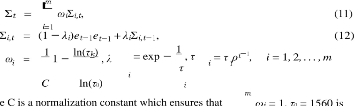
Σt =

m

ωiΣi,t, (11)

i=1

Σi,t = (1 − λi)et−1e_t−1+ λiΣi,t−1, (12)

ω = 11 − ln(τk), λ = exp− 1, τ = τ ρi−1, i = 1, 2, . . . , m

C ln(τ0) _i

m

the d_√ecay parameters, τ1 = 4 is a lower cut-off and τmax = 512 is an upper cut-off,

ρ = 2 is an additional parameter to operationalize the model. Zumbach (2007)

suggested the values to each of the four parameters through forecasting exercises6.

ln ( τmax } According to Sheppard (2013), m = 1 + τ1 ln(ρ)

To summarize all the models we estimate in this study, in table 1 there is the list of model and a brief description of them.

Table 1: List of forecasting models

Name Description

No-change Random Walk: Σˆt+1 = Σt

EWMA Exponentially Weighted Moving Average (λ = 0.97)

Riskmetrics 2006 Riskmetrics methodology 2006

LASSOVAR(1) VAR(1) selecting by LASSO

AdaLASSOVAR(1) VAR(1) selecting by adaptive LASSO

Autometrics VAR(1) VAR(1) selecting by Autometrics

Autometrics VAR(1) DIIS VAR(1) selecting by Autometrics using IIS, SIS and DIS.

LASSOVAR(5) VAR(5) selecting by LASSO

AdaLASSOVAR(5) VAR(5) selecting by adaptive LASSO

Autometrics VAR(5) VAR(5) selecting by Autometrics

Autometrics VAR(5) DIIS VAR(5) selecting by Autometrics using IIS, SIS and DIS

Combination equal Forecast combination - equal weights

Combination weight Forecast combination - weights calculated by equation (9)

Note: VAR(p) means vector autoregressive model of order p. IIS is impulse dummy saturation; SIS is step impulse saturation; DIS is difference impulse saturation. Source: The authors.

3.5 Forecasting evaluation

Let eˆt+h denote vech Σˆ_t+h− Σt+h , where Σˆt+h is the forecast covariance ma-

trix for time period t + h using the methods we described in the previous sections.

6_{As the results for Riskmetrics 1996 and Riskmetrics 2006 are very similar, to save space, we}

show the forecasting error measures for the latter in table A2 in appendix.

τ

i=1

where C is a normalization constant which ensures that ωi = 1, τ0 = 1560 is

. i

(15)

∈ | | t=1 2 H h=1 t+h 1 √

Σt+h is the observed covariance matrix for the same period. The forecast are com-

puted for periods h, where h = 1, . . . , H. In order to evaluate the methods’ perfor- mances, we compute the following indicators:

1. Average g -forecast error (L2): H \eˆ \; 1 2. Average median absolute error (AMedAFE):

H

h=1 median (|eˆt+_h |). It is

more robust to outliers then than g2;

1 3. Average maximal absolute forecast error (AMaxAFE):

H

h=1 max (|eˆt+h|)

We compute all the indicators to the whole forecast covariance matrix and individually for the variance and covariance.

3.5.1 Predictive ability tests

We also apply the model confidence set (MCS) of Hansen et al. (2011) and conditional predictive ability test of Giacomini and White (2006). The MCS consists of an algorithm that selects the best model under some criterion given a level of confidence. In this sense, it is analogous to a confidence interval for a parameter. The advantage of using this procedure is the ability it has to rank all the models given their predictive performance.

MCS uses an equivalence test, δM , to create a set of selected models. Formally, it tests the null hypothesis that H0 : E(di,j) = 0 for all i, j ∈ M where M is a

set of selected models and di,j = g(ei) − g(ej) where gij is some loss function. The alternative hypothesis is given by: H1 : E(di,j) = 0 for all i, j M .

The null hypothesis can be tested using the following statistic which does not have a standard distribution but it can be easily simulated by bootstrap techniques:

TR,M = max tij (13)

i,j∈M where tij = d¯ij

V ar(d¯ij ) and the elimination rule is ρM = arg maxi∈M sup(tj∈M ij) and

d¯ij = H−1 H dij for some i and j. The algorithm works as following: 1. Set the initial set of models M0 ∈ M ;

2. It tests H0 applying δM at a significance level α;

3. If H0 is rejected, it eliminate the object using ρM and it goes back to step

1. The procedure ends when H0 is not rejected. Then, the surviving objects

compose the model confidence set, M1−α;

4. At the end, it uses the p-value to rank the surviving models.

Although the advantage of comparing multiple forecasts and the ability to rank the elements of confidence set, its assumptions may not hold when forecasts are based on estimated parameters Hansen et al. (2011). According to Hansen et al. (2011), some of the problems in this context can be avoid using a rolling window to estimate the parameters, but further modifications are also required. Otherwise, it can

(16)

16

compromise the results, especially when comparing nested models.

To overcome this problem, Giacomini and White (2006) generalized West (1996) and McCracken (2000) to incorporate the use of conditional information, which al-

(17)

τ L L 2

lows to deal with parameter uncertainty and comparison of nested models. Formally, Giacomini and White (2006) tests the null hypothesis that H0 : E(g(yt, f1t(βˆ₁t)) −

g(yt, f2t(βˆ₂t))|It) = 0, where g is loss function, f1t and f2t are two competing mod-

els and, βˆ1t and βˆ2t are its respective estimated parameters. The expectation is

conditioned on the set of information It. The test statistic has the form:

T h = n n−1 T −τ t=m ht∆gm,t+τ Ω˜−_n1 n−1 T −τ t=m ht∆gm,t+τ ∼ χ_q (14)

where τ is the forecast horizon, ∆gm,t−τ = g(yt, f1t(βˆ1t)) − g(yt, f2t(βˆ2t)), n = T − τ ,

ht is a q × 1 It-measurable function. Ω˜ is a consistent estimator of the variance

of ht∆gm,t+τ . When τ > 1, Giacomini and White (2006) argued that ht∆gm,t+τ is

serial correlated, thus, some robust estimator, such as Newey and West (1987) must be used.

This test also requires that the parameters are estimated using a fixed scheme, where it is estimated once and computed all the forecasts, or using a rolling window, which we use in this study. The idea behind this requirement is that this test can handle data that are mixing and heterogeneous (Giacomini and Rossi, 2010).

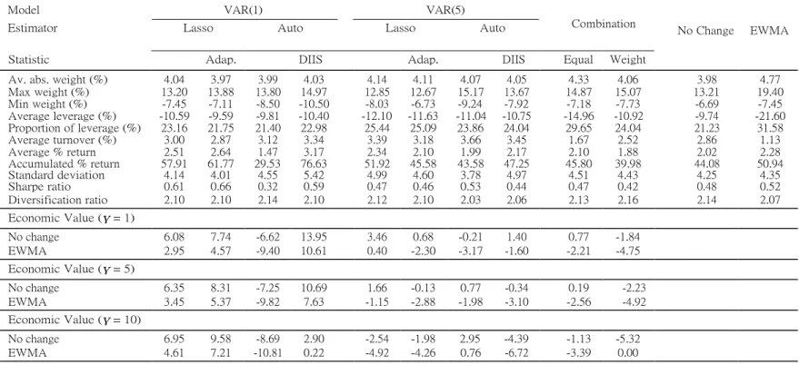
3.5 Portfolio allocation

The portfolio analysis is based on the framework developed by Fleming et al. (2001, 2003) as in Callot et al. (2017). We consider a risk-averse agent that needs to compose his investment portfolio with n = 30 assets. To do so, he uses the mean-variance analysis in every period t of time. He has the utility function given by U (rpt) = (1 + rpt γ ) − 1 + γ (1 + rrt ) 2 ,

where rpt is the portfolio return at time t and γ is investor’s risk averse coefficient. Larger γ means the investor is more risk-averse. We assume γ = 1, 5, 10.

Every period t = t0, . . . , T , the investor decides the vector of weights for the

next period wˆt+1 using information up to t solving the following problem:

wˆt+1 = argmin w_t+1Σˆt+1wt+1 wt+1 s.t. wt+1µˆt+1 = µ n i=1 n i=1 w_{i,t+1 = 1} |wi,t+1|1 (w_it < 0) ≤ 0.30 (15) |wi,t+1| ≤ 0.20,

(18)

18

where wt+1 is n × 1 vector of portfolio weights on the stock, µ is the target return

(19)

· − − ≤ ≤ 1 1 1 nH t=t0 i=1 it nH

of the short position;

t=t0 i=1

nH t=t0 i=1

i,t+1 i,t+1 is the realized return of stock i in time t;

1

by a moving average of the same size of the estimation window for the covariance matrix and 1( ) is a indicator function.

The investor’s problem is to choose the weights for next period’s investment subject to the target return µ and the forecast covariance matrix , Σˆt+1, and returns,

µˆt+1. As in Callot et al. (2017), we also impose the maximum leverage of the

portfolio to be 30% and the maximum weight of one individual asset to be between [ 20%, 20%]. In this setting the problem does not have a closed form solution and it needs to be solved numerically. We also consider as in Brito et al. (2018) a different scenario where short-selling is not allowed, that is, the last restriction becomes 0 wi,t+1 0.20 and the third one does not apply. We set the transaction cost

to 0.1% to both scenarios.

In order to analyze the performance of each forecasting strategy in this exercise, we compute the following statistics7 in which H = T t0 +1 is the number of periods

the investor solves the minimisation problem givem by equations (15): 1. Average absolute weight: T n |wˆ |;

2. Max weight: maxt0≤t≤T max1≤i≤n(wˆit);

3. Min weight: mint0≤t≤T min1≤i≤n(wˆit);

4. Average leverage: T n |w |1 (w < 0), the average of the weights

5. Portfolio leverage: T n 1 (w < 0);

6. Average turnover: T n |w −whold |, where whold = w (1 + rit−1) ,

7. Average return of the portfolio: µ

= T r = T wˆr ; 8. Accumulated return: I TT (1 + rpt); p H t=t0 pt H t=t0 it t t=t_✓0 9. Standard deviation: σp = 10. Sharpe ratio: µp ; σp 1 T H t=t0 _(rpt − µ_p)2_; 1 T 11. Average diversification ratio:

n i=1

wˆitσit

, where σp = wˆt Σitwˆt and

H t=t0 σ

p

σit is the variance of the asset i in time t;

1 where r it p,t−1 ) i,t+1 it it i,t+1 i,t−1 (1 + r

(20)

20 t=t0 t=t0

12. Economic value: The economic value is the value of ∆ such that for different portfolios p1 and p2, we have

T T

L

U (rp1t) =

L

U (rp2t − ∆) . (16)

It represents the maximum return the investor would be willing to sacrifice

(21)

21

switching from p1 to p2. For instance, p1 is either no change forecasting strat-

egy or EMWA.

(22)

22

4 Results

4.1 Analysis of the dynamics and models

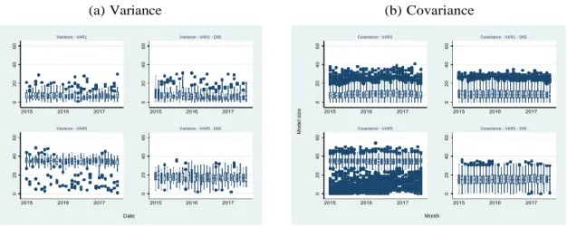
The advantage of those methods is the possibility of analysing the determinants of the covariance matrices and how they vary over time. Thus, in this section we assess the drivers of the dynamic of the selected models for each selection method and period. Figures 1 and 2 display the size of the models for Lasso and Auto- metrics based models for variance (figure a) and covariances (figure b) equations, respectively. The average size of the selected models is quite stable over the period 2015 to 2017 for both selection methods.

Interestingly, Lasso selected from 55 to 80 variables when the model is a VAR(1) and Var(5) and the size is also similar to diagonal and off-diagonal equations. To VAR(5) the models are slight larger. This result is in line with Callot et al. (2017) that find that Lasso selects model twofold bigger for VAR(20) compared to VAR(1) for daily volatility. Of course, there is a difference of magnitude, but our results indicates the same pattern.

Adaptive Lasso behaves as expected. The number of selected variables for each model is almost half of that with Lasso. It is expected due to Lasso is the first stage of the adaptive Lasso. The sizes are also similar to VAR(1) and VAR(5) models. We will explore the differences in drivers later in this study.

Autometrics selects an even sparse array of parameters, due to the fact that this method satisfies the Oracle property, which is not the case for Lasso and adaLasso. The average model size is around 8 variables when the model is a VAR(1) and 35 when it is a VAR(5). The difference in size for the latter is expected as the significance level, α = 0.01 is the same. Autometrics tends to select αK, where K is the number of candidate variables. Theoretically, Autometrics would select 4 variables for VAR(1) and 22 for VAR(5).

With the inclusion of dummy saturation, the average size for VAR(1) model is stable and around 8 as well, but with a higher dispersion. For VAR(5) model, the average size is closer to 22, although the dispersion is also higher. Due to outliers, more relevant variables may have been excluded. Comparing the dispersion of Autometrics and Lasso, the former presents larger variability in models sizes.

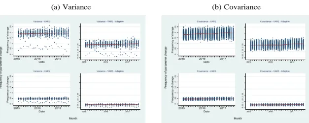
To analyze the stability of the parameters from month to month, figures 3a and 3b plot the frequency of times each variable is selected at period t but not retained at period t+1. Autometrics returns much more stable models, that is, the evolution of the frequency of changes is almost a horizontal line as it can be seen in figures 3a and 3b. The average change in parameters to all equations is below 10%. Interestingly, it is even lower to VAR(5) model and it also presents lower dispersion. For Lasso in figures 4a and 4b, the results are also similar to Callot et al. (2017). The frequency of changes are stable over time but higher than Autometrics models. For Lasso models, they are around 20% for VAR(1) and 5% for VAR(5). The difference between diagonal and off-diagonal equations in terms of changes in parameters is that for the former, the dispersion is higher but the level is lower.

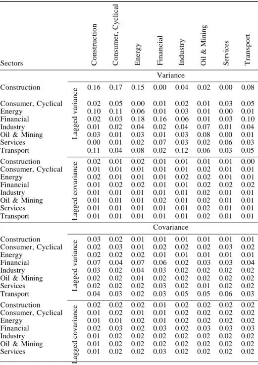
In order to understand better the main driver of the variance and covariance, tables 2 and 3 show the average across estimation windows of the fractions of re-

(23)

Figure 1: Models’ sizes to Lasso and adaptive Lasso

(a) Variance (b) Covariance

Source: The authors.

Figure 2: Models’ sizes to Autometrics

Figure 3: Parameter stability analysis to Autometrics models

Date

Variance - VAR5 - Adaptive Variance - VAR5

Variance - VAR1 - Adaptive Variance - VAR1

Month

Covariance - VAR5 - Adaptive Covariance - VAR5

Covariance - VAR1 - Adaptive Covariance - VAR1

Date

Variance - VAR5 - DIIS Variance - VAR5

Variance - VAR1 - DIIS Variance - VAR1

Month

Covariance - VAR5 - DIIS Covariance - VAR5

Covariance - VAR1 - DIIS Covariance - VAR1

Variance - VAR1 - No DIIS Variance - VAR1 - DIIS

Variance - VAR5 - No DIIS Variance - VAR5 - DIIS

Month

Covariance - VAR1 - No DIIS Covariance - VAR1 - DIIS

Covariance - VAR5 - No DIIS Covariance - VAR5 - DIIS

Month F re q u e n c y o f p a ra m e te r c h a n g e M o d e l s iz e M o d e l s iz e 0 . 0 2 . 0 4 . 0 6 . 0 8 . 1 . 1 2 0 . 0 2 . 0 4 . 0 6 . 0 8 . 1 . 1 2 s iz e 2 0 4 0 6 0 s iz e 2 0 4 0 6 0 0 20 40 60 0 20 40 60 0 80 0 80 0 . 0 2 . 0 4 . 0 6 . 0 8 . 1 . 1 2 0 . 0 2 . 0 4 . 0 6 . 0 8 . 1 . 1 2 s iz e 2 0 4 0 6 0 s iz e 2 0 4 0 6 0 0 20 40 60 0 20 40 60 0 80 0 80 F re q u e n c y o f p a ra m e te r c h a n g e M o d e l s iz e M o d e l s iz e s iz e 2 0 4 0 6 0 s iz e 2 0 4 0 6 0 0 . 0 2 . 0 4 . 0 6 . 0 8 . 1 . 1 2 0 . 0 2 . 0 4 . 0 6 . 0 8 . 1 . 1 2 0 20 40 60 0 20 40 60 0 80 0 80 0 . 0 2 . 0 4 . 0 6 . 0 8 . 1 . 1 2 0 . 0 2 . 0 4 . 0 6 . 0 8 . 1 . 1 2 s iz e 2 0 4 0 6 0 s iz e 2 0 4 0 6 0 0 20 40 60 0 20 40 60 0 80 0 80

(24)

24

Figure 4: Parameter stability analysis to Lasso and adaptive Lasso models

gressors (in rows) from each sector selected to each equation (in columns) from each sector for Autometrics and Lasso VAR(1) models8. This number goes from zero to one and we compute as the average of the number of variables from each category in row divided by the number of all candidates of the same type to each sector in the column.

The results are similar for both types of model selection methods and accord- ingly to what Callot et al. (2017) found for monthly aggregation and Lasso-based forecasts. From table 2 and, to complement from tables A3, A4 and A5 in the appendix, we find that the lagged variance is selected more often for the variance equations. For construction and financial sectors, are more evident from those tables. We see that 16% of the lagged variance of the construction sector is retained in the firms’ models from the same sector using Autometrics (table 2). The fraction for financial sector is also 16%. When we use a VAR(5) A4, those fractions decrease to 5% and 4%, respectively.

With the inclusion of dummy variables, the conclusion changes. Tables A3 and A5 report the results. All lagged variances of all sector are almost equally selected. The exception is finance sector which presents 12% of its own past variances as main drivers in a VAR(1) model. This value changes to 2% when a VAR(5) is used. The lagged covariances do not seem to be important to variance equation in any model. Their selection rate are close to zero.

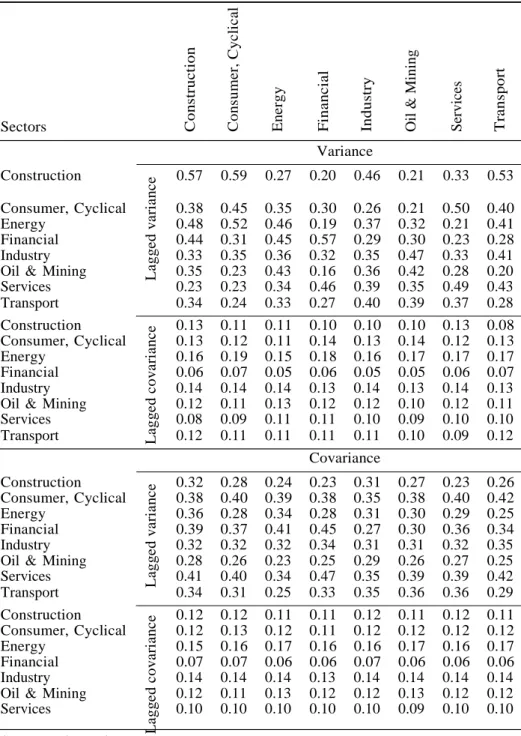
For Lasso based models, we see the same pattern for construction and financial sector though the magnitude of the factions is different. For both, 57% (table 3) of the lagged variance is retained for the diagonal equations for a VAR(1) model and it decreases to 35% and 37%, respectively, when the model is a VAR(5) (table A7). For adaptive Lasso, in tables A6 and A8, those fractions go to below 10%.

For all models, the lagged covariances are little selected to variance equations. This is also found by Callot et al. (2017).

Two points must be highlighted. the first is the difference in fractions between

8_{To save space, the respective tables A3, A4, A5, A6, A7 and A8 for the other models and}

methods are in appendix.

Variance - VAR1 Variance - VAR1 - Adaptive

Variance - VAR5 Variance - VAR5 - Adaptive

Month

Covariance - VAR1 Covariance - VAR1 - Adaptive

Covariance - VAR5 Covariance - VAR5 - Adaptive

Month F re q u e n c y o f p a ra m e te r c h a n g e Fr e q u e n c y o f c h a n g e 0 . 0 5 .1 .1 5 .2 .2 5 Fr e q u e n c y o f c h a n g e 0 . 0 5 .1 .1 5 .2 .2 5 0 . 0 5 . 1 . 1 5 . 2 . 2 5 0 . 0 5 . 1 . 1 5 . 2 . 2 5 F re q u e n c y o f p a ra m e te r c h a n g e Fr e q u e n c y o f c h a n g e 0 . 0 5 .1 .1 5 .2 .2 5 Fr e q u e n c y o f c h a n g e 0 . 0 5 .1 .1 5 .2 .2 5 0 . 0 5 . 1 . 1 5 . 2 . 2 5 0 . 0 5 . 1 . 1 5 . 2 . 2 5

(25)

Source: The authors. L a g ge d c o va ri a nc e L a g ge d va ri a nc e L a g ge d c o va ri a nc e L a g ge d va ri a nc e

Table 2: Fraction of regressors (rows) selected to equations (column) to Autometrics based models Sectors Construction Variance 0.16 0.17 0.15 0.00 0.04 0.02 0.00 0.08 Consumer, Cyclical 0.02 0.05 0.00 0.01 0.02 0.01 0.03 0.05 Energy 0.10 0.11 0.06 0.01 0.03 0.01 0.00 0.01 Financial 0.02 0.03 0.18 0.16 0.06 0.01 0.03 0.10 Industry 0.01 0.02 0.04 0.02 0.04 0.07 0.01 0.04 Oil & Mining 0.03 0.01 0.03 0.01 0.03 0.08 0.00 0.01 Services 0.00 0.01 0.02 0.07 0.03 0.02 0.06 0.03 Transport 0.11 0.04 0.08 0.02 0.12 0.06 0.03 0.05 Construction 0.02 0.01 0.02 0.01 0.01 0.01 0.01 0.00 Consumer, Cyclical 0.01 0.01 0.01 0.01 0.01 0.02 0.01 0.01 Energy 0.02 0.01 0.01 0.01 0.02 0.02 0.01 0.01 Financial 0.01 0.02 0.02 0.01 0.01 0.02 0.02 0.02 Industry 0.01 0.01 0.01 0.01 0.01 0.02 0.01 0.01 Oil & Mining 0.01 0.01 0.01 0.02 0.01 0.02 0.01 0.01 Services 0.01 0.01 0.01 0.01 0.01 0.02 0.01 0.01 Transport 0.01 0.01 0.01 0.01 0.01 0.02 0.01 0.01 Covariance Construction 0.03 0.02 0.01 0.01 0.01 0.01 0.01 0.01 Consumer, Cyclical 0.02 0.03 0.01 0.02 0.02 0.02 0.03 0.02 Energy 0.02 0.02 0.02 0.01 0.01 0.01 0.01 0.01 Financial 0.07 0.04 0.07 0.06 0.02 0.03 0.03 0.04 Industry 0.03 0.02 0.04 0.03 0.02 0.02 0.02 0.02 Oil & Mining 0.02 0.02 0.01 0.02 0.02 0.02 0.02 0.02 Services 0.02 0.02 0.02 0.03 0.02 0.01 0.02 0.02 Transport 0.04 0.03 0.02 0.03 0.05 0.05 0.06 0.03 Construction 0.02 0.02 0.02 0.01 0.02 0.02 0.02 0.02 Consumer, Cyclical 0.01 0.02 0.01 0.01 0.02 0.02 0.02 0.02 Energy 0.01 0.01 0.02 0.01 0.02 0.02 0.02 0.02 Financial 0.02 0.03 0.02 0.03 0.02 0.03 0.03 0.03 Industry 0.01 0.02 0.02 0.02 0.02 0.02 0.02 0.02 Oil & Mining 0.01 0.02 0.02 0.02 0.02 0.02 0.02 0.02 Services 0.01 0.02 0.02 0.03 0.02 0.02 0.02 0.02 C o n str u ct io n C o ns u m e r, C yc li c al E ne rg y F in a n c ial In d u st ry Oil & Min in g Ser v ices T ra n sp o rt

(26)

19

(27)

Source: The authors. L a g ge d c o va ri a nc e L a g ge d va ri a nc e L a g ge d c o va ri a nc e L a g ge d va ri a nc e

Table 3: Fraction of regressors (rows) selected to equations (column) to Lasso based models Sectors Construction Variance 0.57 0.59 0.27 0.20 0.46 0.21 0.33 0.53 Consumer, Cyclical 0.38 0.45 0.35 0.30 0.26 0.21 0.50 0.40 Energy 0.48 0.52 0.46 0.19 0.37 0.32 0.21 0.41 Financial 0.44 0.31 0.45 0.57 0.29 0.30 0.23 0.28 Industry 0.33 0.35 0.36 0.32 0.35 0.47 0.33 0.41 Oil & Mining 0.35 0.23 0.43 0.16 0.36 0.42 0.28 0.20 Services 0.23 0.23 0.34 0.46 0.39 0.35 0.49 0.43 Transport 0.34 0.24 0.33 0.27 0.40 0.39 0.37 0.28 Construction 0.13 0.11 0.11 0.10 0.10 0.10 0.13 0.08 Consumer, Cyclical 0.13 0.12 0.11 0.14 0.13 0.14 0.12 0.13 Energy 0.16 0.19 0.15 0.18 0.16 0.17 0.17 0.17 Financial 0.06 0.07 0.05 0.06 0.05 0.05 0.06 0.07 Industry 0.14 0.14 0.14 0.13 0.14 0.13 0.14 0.13 Oil & Mining 0.12 0.11 0.13 0.12 0.12 0.10 0.12 0.11 Services 0.08 0.09 0.11 0.11 0.10 0.09 0.10 0.10 Transport 0.12 0.11 0.11 0.11 0.11 0.10 0.09 0.12 Covariance Construction 0.32 0.28 0.24 0.23 0.31 0.27 0.23 0.26 Consumer, Cyclical 0.38 0.40 0.39 0.38 0.35 0.38 0.40 0.42 Energy 0.36 0.28 0.34 0.28 0.31 0.30 0.29 0.25 Financial 0.39 0.37 0.41 0.45 0.27 0.30 0.36 0.34 Industry 0.32 0.32 0.32 0.34 0.31 0.31 0.32 0.35 Oil & Mining 0.28 0.26 0.23 0.25 0.29 0.26 0.27 0.25 Services 0.41 0.40 0.34 0.47 0.35 0.39 0.39 0.42 Transport 0.34 0.31 0.25 0.33 0.35 0.36 0.36 0.29 Construction 0.12 0.12 0.11 0.11 0.12 0.11 0.12 0.11 Consumer, Cyclical 0.12 0.13 0.12 0.11 0.12 0.12 0.12 0.12 Energy 0.15 0.16 0.17 0.16 0.16 0.17 0.16 0.17 Financial 0.07 0.07 0.06 0.06 0.07 0.06 0.06 0.06 Industry 0.14 0.14 0.14 0.13 0.14 0.14 0.14 0.14 Oil & Mining 0.12 0.11 0.13 0.12 0.12 0.13 0.12 0.12 Services 0.10 0.10 0.10 0.10 0.10 0.09 0.10 0.10 C o n str u ct io n C o ns u m e r, C yc li c al E ne rg y F in a n c ial In d u st ry Oil & Min in g Ser v ices T ra n sp o rt

(28)

21

(29)

selection methods which may be explained by the difference in size previously dis- cussed. As Lasso does not select through hypothesis testing, there may be more non-significant variables retained, what may be beneficial for prediction as it may reduce the forecasting error. The second is the replacement from lagged variance to lagged covariance when the order of the VAR model increases as reported in tables A6, A7 and A8 in appendix. For instance, for Consumer cyclical sector and VAR(1) in table 2, the relation between fractions of the lagged variance and covariance in the variance equation is 5 while it reduces to 3 for a VAR(5) in table A4.

For the covariance equations, the conclusions are also similar between all models and selection methods. The lagged variances are more retained than the lagged covariance, but the difference in fractions is not large. It means that the past variance is relatively more important to the covariances models. We must also note that there are 435 equations, the number of firms is different among sectors and each covariance between two stocks enters in two different rows, so interpretation is not trivial.

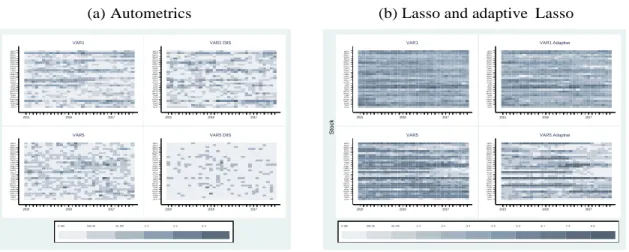
In order to explore more the determinants of the variances equations, we plot in figure 5 the percentage of times the lagged variance is retained for each variance equation of each stock in each period. For Autometrics (panel a), the past variance is more retained for VAR(1), especially to Banco do Brazil (BBSA3) and Cyrela (CYRE3) stocks, close to 40%. With the inclusion of dummy saturation, the selection rate reduces, but it is still relatively high to BBSA3. For VAR(5), the past variances are selected less than 10% to most of the stocks.

For Lasso based models, panel b, there is a different conclusion. The past variances are highly selected to most of the periods and stocks, close 90%. Especially for VAR(1), on the top left of panel a. For adaptive LASSO VAR(5) at the end of the period, it seems to change and less lagged variances are selected.

Figure 5: Selection frequency of the diagonal equations

(a) Autometrics (b) Lasso and adaptive Lasso

To conclude, both methods show the importance of the lagged variances to the diagonal and off-diagonal equations, besides the differences in the level of retention. It also seems that extreme values may induce the selection of those variables as, using dummy saturation strategy, the selection rate of the past variances reduces to all equations and periods. The differences in size may be explained by the low

0-.025 .025-.05 .05-.075 .1-.2 .2-.3 .3-.4 2017 2016 2015 2017 2016 2015 VAR5 DIIS VAR5 2017 2016 2015 2017 2016 2015 VAR1 DIIS VAR1 0-.025 .025-.05 .05-.075 .1-.2 .2-.3 .3-.4 .4-.5 .5-.6 .6-.7 .7-.8 .8-.9 2017 2016 2015 2017 2016 2015 VAR5 Adaptive VAR5 2017 2016 2015 2017 2016 2015 VAR1 Adaptive VAR1 St o c k St o c k

(30)

21

{ }

significance level we adopt to Autometrics. Increasing the significance level would yield larger models. Autometrics also returns more stable models, that is, the change in selected variables between periods is lower. Besides the opportunity to explore the drivers of the covariance matrix of the selected stocks, this paper aims to compare their forecasting performance what is done in the next sections.

4.2 Forecasting Evaluation

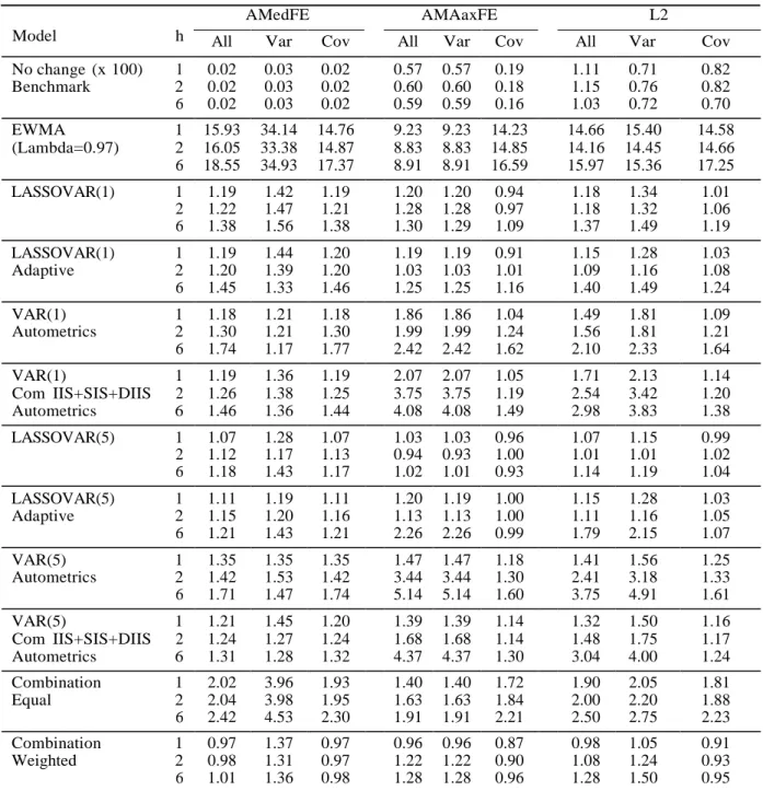
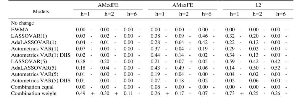
In this section, we forecast the covariance matrix using each selection method and analyse their performance over different horizons: one, two and six months ahead. Table 4 reports the three forecasting error measures, respectively, the average maximal absolute error (AMaxFE), the average median absolute error (AMedFE) and the average g2 error (L2), for the variance (VAR), covariances (Cov) and all the matrix

(All). All values are in relation to the benchmark model, no change. If the number is above one, it means the model is not able to deliver better forecasts than the benchmark.

Table 4 shows that it is very hard to an individual model to beat the benchmark. For all forecasting horizons and error measures the no-change model delivers more accurate predictions. EWMA and Riskmetrics 2006 under-perform by far all models (see table A2 in appendix). Our results are in accordance to Callot et al. (2017) for monthly data.

The equal forecast combination does seem to be very affected by the worse forecasts, specifically EWMA, and it also performs poorly. The weighted combination of forecast, however, is able to beat the benchmark for all horizons and forecast error measures. Specifically, it is more precise for the next month and two periods ahead,

h = 1, 2 , respectively. The level of improvement over the benchmark de- pendents

on the forecast error measures. For AMedFE, the forecasts are up to 3% more precise for the whole matrix and covariance equations. Using the AMaxFE, there is a gain of 13% over the no-change forecast for the covariance equation one step ahead (h = 1) and 10% for h = 2. The variance, the combination outperforms in 4% in the shortest horizon. In the longest, the gain is smaller, 4%. For L2, the weighted combination is more precise up to 9% for the off-diagonal equations. Cava- leri and Ribeiro (2011) also found improvements using different types of forecasting combinations to Ibovespa index volatility.

Differently from Callot et al. (2017), our results show that the covariances are more precisely forecast than the variances. This outcome is robust to horizons and forecast error measures. The improvement seems to be slightly larger using the average maximum forecast error (AMaxFE).

It is also worth noting that among LASSOVAR models, the adaptive LASSO- VAR(1) and LASSOVAR(1) have similar performance, while for VAR(5), LASSO- VAR outperforms adaptive LASSOVAR. As we note in the previous section, it may be explained by the number of variables retained in each model. While retaining more variable reduces the forecasting error, it also increases its variance.

When the model selection is Autometrics, the performance is similar for a VAR(1) with and without dummy saturation. For a VAR(5) model, the inclusion of dummy saturation is beneficial and there is an increase in precision to all fore-

(31)

Table 4: Forecast error measures

AMedFE AMAaxFE L2

Model h _All _Var _Cov _All _Var _Cov _All _Var _Cov

No change (x 100) 1 0.02 0.03 0.02 0.57 0.57 0.19 1.11 0.71 0.82 Benchmark 2 0.02 0.03 0.02 0.60 0.60 0.18 1.15 0.76 0.82 6 0.02 0.03 0.02 0.59 0.59 0.16 1.03 0.72 0.70 EWMA 1 15.93 34.14 14.76 9.23 9.23 14.23 14.66 15.40 14.58 (Lambda=0.97) 2 16.05 33.38 14.87 8.83 8.83 14.85 14.16 14.45 14.66 6 18.55 34.93 17.37 8.91 8.91 16.59 15.97 15.36 17.25 LASSOVAR(1) 1 1.19 1.42 1.19 1.20 1.20 0.94 1.18 1.34 1.01 2 1.22 1.47 1.21 1.28 1.28 0.97 1.18 1.32 1.06 6 1.38 1.56 1.38 1.30 1.29 1.09 1.37 1.49 1.19 LASSOVAR(1) 1 1.19 1.44 1.20 1.19 1.19 0.91 1.15 1.28 1.03 Adaptive 2 1.20 1.39 1.20 1.03 1.03 1.01 1.09 1.16 1.08 6 1.45 1.33 1.46 1.25 1.25 1.16 1.40 1.49 1.24 VAR(1) 1 1.18 1.21 1.18 1.86 1.86 1.04 1.49 1.81 1.09 Autometrics 2 1.30 1.21 1.30 1.99 1.99 1.24 1.56 1.81 1.21 6 1.74 1.17 1.77 2.42 2.42 1.62 2.10 2.33 1.64 VAR(1) 1 1.19 1.36 1.19 2.07 2.07 1.05 1.71 2.13 1.14 Com IIS+SIS+DIIS 2 1.26 1.38 1.25 3.75 3.75 1.19 2.54 3.42 1.20 Autometrics 6 1.46 1.36 1.44 4.08 4.08 1.49 2.98 3.83 1.38 LASSOVAR(5) 1 1.07 1.28 1.07 1.03 1.03 0.96 1.07 1.15 0.99 2 1.12 1.17 1.13 0.94 0.93 1.00 1.01 1.01 1.02 6 1.18 1.43 1.17 1.02 1.01 0.93 1.14 1.19 1.04 LASSOVAR(5) 1 1.11 1.19 1.11 1.20 1.19 1.00 1.15 1.28 1.03 Adaptive 2 1.15 1.20 1.16 1.13 1.13 1.00 1.11 1.16 1.05 6 1.21 1.43 1.21 2.26 2.26 0.99 1.79 2.15 1.07 VAR(5) 1 1.35 1.35 1.35 1.47 1.47 1.18 1.41 1.56 1.25 Autometrics 2 1.42 1.53 1.42 3.44 3.44 1.30 2.41 3.18 1.33 6 1.71 1.47 1.74 5.14 5.14 1.60 3.75 4.91 1.61 VAR(5) 1 1.21 1.45 1.20 1.39 1.39 1.14 1.32 1.50 1.16 Com IIS+SIS+DIIS 2 1.24 1.27 1.24 1.68 1.68 1.14 1.48 1.75 1.17 Autometrics 6 1.31 1.28 1.32 4.37 4.37 1.30 3.04 4.00 1.24 Combination 1 2.02 3.96 1.93 1.40 1.40 1.72 1.90 2.05 1.81 Equal 2 2.04 3.98 1.95 1.63 1.63 1.84 2.00 2.20 1.88 6 2.42 4.53 2.30 1.91 1.91 2.21 2.50 2.75 2.23 Combination 1 0.97 1.37 0.97 0.96 0.96 0.87 0.98 1.05 0.91 Weighted 2 0.98 1.31 0.97 1.22 1.22 0.90 1.08 1.24 0.93 6 1.01 1.36 0.98 1.28 1.28 0.96 1.28 1.50 0.95 Note: The number for No-change are in absolute values and the others are relative to the benchmark. All: All the covariance matrix; Var: only the variance; Cov: only the covariance. We forecast h months ahead where h = 1, 2, 6.

(32)

23

casting horizons, with some exceptions, for example, variance forecast 1 step ahead with increases from 35

Comparing Autometrics and LASSO, we note that for a VAR(1), the performance is quite similar while LASSO and adaptive LASSO outperform Autometrics we use VAR(5) model. It is worth noting that the tendency of VAR(5) forecast better than the VAR(1) may be a consequence of the long memory characteristics presented in volatility series (Granger et al., 2000, for instance).

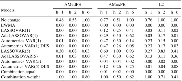
In order to check the statistically differences in the models’ forecast, we calculate the Model Confidence Set (Hansen et al., 2011) and Giacomini and Rossi (2010)’s conditional test. The results are in tables 5 and 6, respectively.

Table 5: Model Confidence Set for all equations

AMedFE AMaxFE L2 Models _h=1 _h=2 _h=6 _h=1 _h=2 _h=6 _h=1 _h=2 _h=6 No change 0.48 0.53 1.00 0.77 0.51 1.00 0.76 1.00 1.00 EWMA 0.00 0.00 0.00 0.00 0.00 0.00 0.00 0.00 0.00 LASSOVAR(1) 0.00 0.00 0.00 0.12 0.25 0.41 0.03 0.11 0.02 AdaLASSOVAR(1) 0.00 0.00 0.00 0.29 0.50 0.62 0.03 0.17 0.01 Autometrics VAR(1) 0.01 0.00 0.00 0.47 0.30 0.14 0.23 0.15 0.00 Autometrics VAR(1) DIIS 0.00 0.00 0.00 0.47 0.26 0.05 0.23 0.17 0.03 LASSOVAR(5) 0.30 0.08 0.03 0.69 1.00 0.93 0.27 0.83 0.41 AdaLASSOVAR(5) 0.01 0.03 0.00 0.47 0.30 0.62 0.13 0.11 0.36 Autometrics VAR(5) 0.00 0.00 0.00 0.04 0.04 0.02 0.00 0.02 0.00 Autometrics VAR(5) DIIS 0.00 0.00 0.00 0.12 0.26 0.25 0.01 0.04 0.08 Combination equal 0.00 0.00 0.00 0.01 0.02 0.00 0.00 0.00 0.00 Combination weight 1.00 1.00 0.80 1.00 0.50 0.62 1.00 0.71 0.41 Note: The table displays the p-values of the MCS. We forecast h = 1, 2, 6 months ahead. Source: The authors.

The MCS depends on the error measure, but still either the weighted combination or the no-change models is the winner. One exception is LASSOVAR(5) for AMaxFE and h = 2. For the average median forecasting error (AMedFE) the weighted combination delivers the most precise predictions for h = /1, 2/. For the h = 6, the final set is composed of the former and the no-change forecast.

The model confidence sets using the average maximal forecasting error (AMaxFE) have more elements than using the previous measure. The ranking is also different depending on the horizon. For one month ahead, the best predictions are from the weighted combination approach followed no-change forecast. For the two months ahead, the winner is LASSOVAR(5) followed by the no-change forecast and weighted combination. For h = 6, the benchmark comes first and LASSOVAR(5) delivers the second most accurate predictions, while the weighted combination ranks in third. Callot et al. (2017) also found Lasso based prediction are more precise in longer horizons and forecasting error measure. This measure is important as they derived the theoretical upper limit of the covariance matrix forecasting error.

Using the last error measure, L2, the weighted combination shows better pre- dictions for h = 1, while the benchmark is in the second. For h = /2, 6/, those models change the position.