EVALUATION OF NON-LINEAR TAPER EQUATIONS FOR PREDICTING THE
DIAMETER OF EUCALYPTUS TREES
1Guilherme Silverio Aquino de Souza*², Diogo Nepomuceno Cosenza², Ana Carolina da Silva Cardoso Araújo³, Lucas Veiga Ayres Pimenta4, Ramon Barreto Souza5, Filipe Monteiro Almeida3 and Helio Garcia
Leite6
1 Received on 03.11.2015 accepted for publication on 28.06.2017.
2 Universidade Federal de Viçosa, Programa de Pós-Graduação em Ciência Florestal, Viçosa, Minas Gerais - Brasil. E-mail:
<guilhermesas.eng@gmail.com>and <dncosenza@gmail.com>.
3 Universidade Federal dos Vales do Jequitinhonha e Mucuri, Doutorado em Ciência Florestal , Diamantina, Minas
Gerais-Brasil. E-mail: <anascaraujo@gmail.com>.
4 Universidade Federal de Viçosa, Programa de Pós-Graduação em Genética e Melhoramento, Viçosa, Minas Gerais - Brasil.
E-mail: <lucasfip@yahoo.com.br>.
5 Universidade Federal de Viçosa, Graduado em Engenharia Florestal, Viçosa, Minas Gerais - Brasil. E-mail: <rabarretoso@gmail.com>
and <filipema@gmail.com>.
6Universidade Federal de Viçosa, Departamento de Engenharia Florestal, Viçosa, Minas Gerais - Brasil. E-mail: <hgleite@ufv.br>.
*Corresponding author.
ABSTRACT – This study aims to evaluate non-linear stem taper models for predicting the pre-commercial diameter of eucalyptus trees and to analyze the effect of genotype on stem taper. The treatments comprise three different genotypes of Eucalyptus sp. in a 3 × 3 m plantation spacing. Seventy sample trees aged 10 years were felled for each treatment. The outside bark diameter measurements were taken at 0.5 m; 1.0 m; 1.5 m; 2.0 m, and then at intervals of 2.0 m till the top of the stem. Four non-linear models were evaluated, namely, the sigmoid model of Garay (1979), the variable exponent model of Kozak (1988), the segmented model of Max and Burkhart (1976), and the compatible model of Demaerschalk (1972). The performance of the models was assessed using the following statistical validation methods: correlation coefficient, standard error of estimate, mean bias, bias variance, root mean squared error, and mean absolute deviation. Graphical analysis of residues was used to evaluate the accuracy and precision of the estimates. Compared with other models, the variable exponent model of Kozak (1988) best described the stem profile, and predicted the total volume of the trees. The identity test showed that the stem profile is affected by the genotype. Keywords: Regression analysis; Variable exponent model; Genotypes
AVALIAÇÃO DE FUNÇÕES DE AFILAMENTO NÃO-LINEARES PARA
ESTIMAÇÃO DE DIÂMETROS COMERCIAIS EM ÁRVORES DE EUCALIPTO
RESUMO – Este trabalho teve como objetivo a escolha de um modelo de afilamento para melhor estimar o perfil médio de árvores de diferentes clones de eucalipto, verificando se uma mesma função pode ser empregada para três genótipos distintos de eucalipto. Os tratamentos consistiram em diferentes clones de eucalipto plantados sob o espaçamento de 3 x 3 m. Para cada tratamento foram abatidas cerca de 70 árvores-amostra aos 10 anos de idade. Os diâmetros das seções ao longo do fuste foram medidos a partir da base em 0.5 m; 1.0 m; 1.5 m; 2.0 m e, a partir daí, em intervalos de 2.0 m. Foram testados quatro modelos não-lineares: Garay (1979), Kozak (1988), Max e Burkhart (1976) e Demaerschalk (1972). As estatísticas utilizadas para avaliar os ajustes foram: coeficiente de correlação entre diâmetros observados e estimados, erro-padrão residual, bias (média dos erros), variância do bias, raiz quadrada do erro quadrático médio e a média das diferenças absolutas. O modelo escolhido para representar os tratamentos, pela melhor performance de ajuste, foi o de Kozak (1988). Testes de identidade de modelo foram aplicados para verificar igualdade no formato do fuste entre os tratamentos. Com base nos resultados, a hipótese de igualdade na forma do fuste dos genótipos foi rejeitada, ao nível de 5% de significância. Assim, pôde-se concluir, que existe efeito do genótipo no afilamento do fuste de eucalipto.
1.INTRODUCTION
The term ‘taper’ was defined by Husch et al. (1993) to describe the rate of diameter decrease in the stem of a tree. Taper equations or functions can predict the narrowing rate or diameter along the bole, which make them very useful techniques for wood assortments. Höjer (1903) conducted the first studies on tree taper. Thereafter, two noteworthy studies by Kozak et al. (1969) and Demaerschalk (1972) were published. Research on stem taper of trees in Brazil began in the early 1970s in Pinus and eucalyptus forest plantations (Silva, 1974; Campos and Ribeiro, 1982; Guimarães and Leite, 1992; Schneider et al., 1996).
Predicting the diameter along the base of the stem is one of the greatest challenges of taper functions given the presence of geometric distortions in this portion (Kozak, 2004; Souza et al., 2008). Based on the variation of geometrical shapes, Max and Burkhart (1976) proposed a model that divides the stem into three sections expressed using three separate sub-models, which together represent the global taper equation. The same basic concept introduced a range of segmented taper equations (Demaerschalk and Kozak, 1977; Parresol et al., 1987). Currently, there exist several models that describe the stem form of trees, and they are broadly categorized into two groups: segmented and non-segmented taper equations. Non-segmented taper equations are classified as polynomial, sigmoid, compatible, or incompatible (Lima, 1986; Pereira et al., 2005; Campos and Leite, 2013). They may also be defined using multivariate analysis (Guimarães and Leite, 1992). Compatible models show consistency between their taper and volume predictions, where the taper equations are the first derivative of the volume equations. Segmented models consider the sectioning of the stem resulting in a more detailed form description (Lima, 1986; Garcia et al., 1993). The variable exponent (Kozak, 1988) and sigmoid models include inflection points that enable them to outline bole diameters that are near the ground more appropriately. The variable exponent model of Kozak (1988) assumes one inflection point (at 0.25 of the total height) and an exponential pattern of decreasing diameter sizes from the tree bottom to top. The sigmoid taper functions are based on biological growth models so that they can describe the natural shape of the tree trunks (Lima, 1986; Muhairwe, 1999).
Present studies have explored a range of taper functions having significant variation in their
performances and results when applied on empirical data. There exist unique functions that, for a particular genotype, outperform the different models, but these yield biased predictions in other instances (Morley and Little, 2012) and thus cannot be universally applied. Several taper functions can generate satisfactory results for most cases in terms of prediction accuracy (Andrade, 2014), which makes assessment a complex task.
Two desirable properties are required in a taper model: the diameter at the maximum height should be null, and the diameter at 1.3 m should be equal to the field measurements of the diameter at breast height (DBH) (Campos and Leite, 2013). Weiskittell et al. (2011) highlighted that comparative studies of taper functions based only on modeling performances are not justifiable, and a biological explanation for the phenomena is important in selecting the appropriate equation. The present study explored well-established taper models that could provide a biological explanation. Therefore, we aimed to compare the non-linear taper models in predicting the pre-commercial diameter of eucalyptus trees, and verify if the same taper model could be employed for three distinct eucalyptus genotypes.
2.MATERIAL AND METHODS
The dataset used in this study comprises trees sampled from eucalyptus stands located at the Bahia state in Brazil. Seventy sample trees (aged 10 years) of each genotype were harvested, constituting three treatments: genotype 1 (G1), genotype 2 (G2), and genotype 3 (G3). The plantation spacing was similar (3 × 3 m) for all treatments. The sampled trees presented a minimum and maximum DBH of 6 cm and 30 cm, respectively, and the total height ranged between 12–42 m.
The four non-linear taper models tested in each genotype were as follows: the sigmoid model of Garay (1979), the Kozak (1988) variable exponent model, the segmented model of Max and Burkhart (1976), and the compatible model of Demaerschalk (1972). These models are given below.
Garay (1979):
d = DBH {0[1+11n(1-2h13H-3)]}+
Kozak (1988):
Max and Burkhart (1976):EQ3
Demaerschalk (1972): EQ4
Here, d denotes the estimated diameter (cm) at hi height; H denotes the total tree height (m); DBH denotes the diameter (cm) at 1,3 m; 0, 1, 2, 0,
1, 2, 3, 4, 5 denote the model parameters to be estimated; Z = hi/H, p = 0.25, e denotes the Napier's constant; denotes the random error, which is ~ N(0,²); and I1 and I2 denote conditional variables where:
I1 = 1, if 1-Z > 0; I1 = 0, if 1-Z < 0; I2 = 1, if 2-Z > 0; I2 = 0, if 2-Z < 0.
The models were fitted using the quasi-Newton optimization algorithm implemented in STATISTICA 12.0 (2014) software. For each fitted model, the following statistics were calculated: correlation coefficient between the observed and predicted values (rYY), standard deviation
(syx), bias, bias variance (s2
bias), root mean squared error (RMSE), and mean absolute deviation (MAD) (Islam et al., 2009; Campos and Leite, 2013):
Here, n denotes the number of observations; p denotes the number of coefficients or parameters; Yi denotes the ith observed value; Yi denotes the ith estimated value; Y denotes the mean of the observed values, and Ym denotes the mean of the estimate Yi. The assessment of the fitted models compared their ability to estimate the diameter along the stem using fit statistics and graphical residual analysis. The models were further tested for their ability to predict individual tree volumes in different DBH
Given that the parameters of the outperformed model were obtained for each genotype, they were compared based on the model identity test proposed by Regazzi and Silva (2004). This method verified if different non-linear regression lines could be combined based on the following definitions:EQ6
(Complete Model) (Reduced Model)
Here, y denotes the d vector of the dependent or response variables;x denotes the vector of the explanatory variables of the complete and reduced models; ƒ denotes the non-linear function; qi denotes the vector of the unknown parameters to each i treatment; h represents the number of equations (comparative cases); Di = 1 and Di = 0, to each treatment i = {1, …, h}, i’ = {1, …, h} being i i’; q denotes the vector of the unknown parameters of the reduced models (combined data) tested under the normality
SQR(H0) = SQPar(R) – SQPar(C); SQPar(C) = yi2 – (y
h – wh)2 SQPar(R) = yr2 – (y
r – wr)2 GLR(H0) = GLC – GLR GLRes = n – p.H Ftab = F(GLR(H0); GLRes)
Here, SQR(H0) denotes the squared sum of reduction because of the null hypothesis (H0); SQPar(C) denotes the squared sum of parameters of the complete model; SQPar(R) denotes the squared sum of parameters of the reduced model; SQRes(C) denotes the squared sum of residues of the complete model; denotes the significance level; GLR(H0) denotes the degrees of freedom of reduction because of the H0 hypothesis; and GLRes denotes the degrees of freedom of residues. If F > Ftab, a significant difference exists among the stem form of the compared genotypes.
3.RESULTS
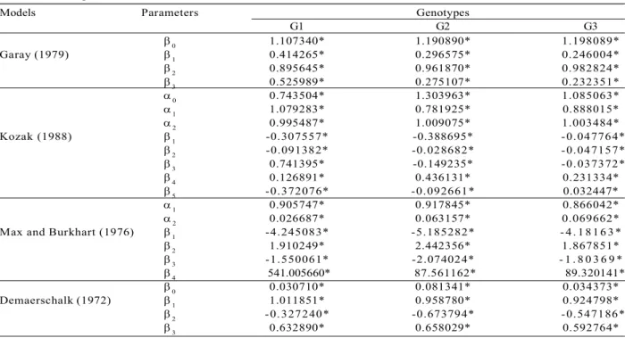
The model parameters were estimated at 5% significance level (Table 1). All models obtained acceptable fit statistics to the data of the different treatments, yielding rYY values up to 0.9 and low standard errors (syx) ranging between 3–7% (Table 2).
^
^
^ ^
=/ d = 10β0DBHβ1H2ß2(H-h)2ß3+
^
^
EQ5
The Kozak (1988) model presented the highest correlation coefficient (rYY) values and the lowest values of bias, indicating the most accurate model to fit the data. The statistics in the precision of estimates, syx (%), did not show a large variation throughout the
assessment. However, the Kozak (1988) variable exponent model and the segmented model of Max and Burkhart (1976) showed the most precise results, whereas the compatible model of Demaerschalk (1972) presented the lowest precision for the three genotypes.
Models Parameters Genotypes
G1 G2 G3
0 1.107340* 1.190890* 1.198089*
Garay (1979) 1 0.414265* 0.296575* 0.246004*
2 0.895645* 0.961870* 0.982824*
3 0.525989* 0.275107* 0.232351*
0 0.743504* 1.303963* 1.085063*
1 1.079283* 0.781925* 0.888015*
2 0.995487* 1.009075* 1.003484*
Kozak (1988) 1 -0.307557* -0.388695* -0.047764*
2 -0.091382* -0.028682* -0.047157*
3 0.741395* -0.149235* -0.037372*
4 0.126891* 0.436131* 0.231334*
5 -0.372076* -0.092661* 0.032447*
1 0.905747* 0.917845* 0.866042*
2 0.026687* 0.063157* 0.069662*
Max and Burkhart (1976) 1 -4.245083* -5.185282* - 4. 1 816 3*
2 1.910249* 2.442356* 1.867851*
3 -1.550061* -2.074024* - 1 . 8 0 3 6 9 *
4 541.005660* 87.561162* 89.320141*
0 0.030710* 0.081341* 0.034373*
Demaerschalk (1972) 1 1.011851* 0.958780* 0.924798*
2 -0.327240* -0.673794* -0.547186*
3 0.632890* 0.658029* 0.592764*
Table 1 – Parameter estimates of four non-linear taper models for comparison with three eucalyptus genotypes.
Tabela 1 – Estimativa dos parâmetros dos quatro modelos de afilamento não-lineares ajustados para três genótipos de
eucalipto.
Onde: * = Significant at 5% probability; k, k = Estimated Model Parameters.
Model Genotype Fit statistics
rYY syx (%) Bias (%) Bias (cm) s2
bias MAD (cm)
Garay (1979) G1 0.995 4.577 0.080ns 0.011ns 0.396 0.462
G2 0.995 4.890 - 0 . 3 5 2* 0.043* 0.360 0.460
G3 0.994 5.363 - 0 . 3 4 9* 0.044* 0.447 0.513
Kozak (1988) G1 0.997 3.934 0.017ns 0.002ns 0.293 0.395
G2 0.996 4.551 0.018ns 0.002ns 0.313 0.417
G3 0.994 4.995 0.037ns 0.005ns 0.389 0.460
Max and Burkhart G1 0.996 4.195 0.092* 0. 013* 0.333 0.424
(1976) G2 0.995 4.883 - 0 . 3 7 2* 0.046* 0.359 0.465
G3 0.994 5.085 - 0 . 3 5 6* 0.044* 0.402 0.487
Demaerschalk (1972) G1 0.995 4.833 0.030ns 0.004ns 0.442 0.447
G2 0.993 5.795 - 0 . 0 9 7* 0.012* 0.508 0.504
G3 0.992 6.143 0.001ns 0.001ns 0.589 0.520
Table 2 – Fit statistics of four non-linear models for three eucalyptus genotypes.
Tabela 2 – Estatísticas de Qualidade de Ajuste das quatro equações ajustadas para três genótipos de eucalipto.
Where, rvY = correlation coefficient; syx = standard error of estimate; s²bias = bias variance; MAD = mean absolute deviation;* = significantly
different from zero at 5% probability by one sample t-test; ns = significantly equal to zero at 5% probability by one sample t-test.
^
We tested bias using a one-sample t-test at 5% significance level to verify its equality from zero (Table 2). This test evaluates the significant difference between the calculated or resulted bias (mean error) and a mean value equal to 0 (null hypothesis), considering bias or error variance (s2
bias) and repetitions of each case (Islam et al., 2009). This assessment resulted in non-significant values of bias for all treatments in Kozak (1988). In contrast, the bias in the segmented model of Max and Burkhart (1976) is statistically different from zero for all cases.
The bias consists in a good statistic for accuracy assessment, but it should be interpreted carefully. For example, the resulting predictions in a modeling process can overestimate certain regions of the dataset, whereas underestimation can occur in other sections. The resulting values of bias can move closer to zero given that opposite trends cancel each other. To overcome this impasse, Muhairwe (1999) suggested MAD for a more correct interpretation of prediction errors. In the present study, MAD values vary between 0.4 and 0.6 cm. For G1, the sigmoid model of Garay (1979) showed the highest MAD values. Similarly, the compatible model of Demaerschalk (1972) presented the highest values for G2 and G3. High values of these statistics indicate a broader range of error dispersion of estimates.
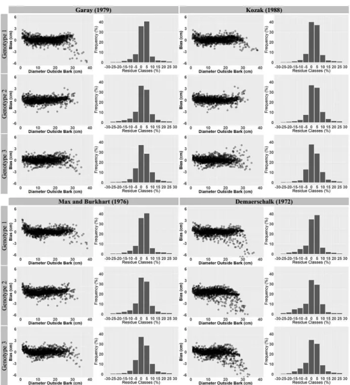
The analysis of residual dispersion of the models tested (Figure 1) showed errors along the different sections of the stem, given that the largest and smallest diameter can be found at the bottom and top of the stem, respectively. The compatible model of Demaerschalk (1972) presented the greatest dispersion of errors for all treatments. The sigmoid model of Garay (1979) presented the greatest diameter estimate error for G1, whereas good performances could be observed for G2 and G3. For all treatments relative to the compatible and sigmoid models, the segmented model of Max and Burkhart (1976) and the Kozak (1988) variable exponent model showed better potential for diameter prediction, especially for the largest diameter, and concentrating the errors closer to zero. The good fit of the two models can be observed in the graphical representation of case percentage per residue classes (Figure 1), where they presented the highest percentage of cases around the classes of 0%.
Despite the large number of errors in diameter prediction, the compatible model of Demaerschalk (1972) did not show the same inaccuracy in predicting the
total volume of trees for all genotypes (Table 3). The compatible model along with the Kozak (1988) variable exponent model showed the most accurate predictions for individual volume in all size classes. For G3 and G4, all models underestimated the small trees, and the most excessive negative bias is presented by the segmented model of Max and Burkhart (1976) and the sigmoid model of Garay (1979).
Given that the variable exponent taper equation had outperformed the estimation of diameters and individual volumes, and its operational convenience of fitting in the segmented models, the Kozak (1988) variable exponent model was chosen for further tests of treatment effects on the tree bole.
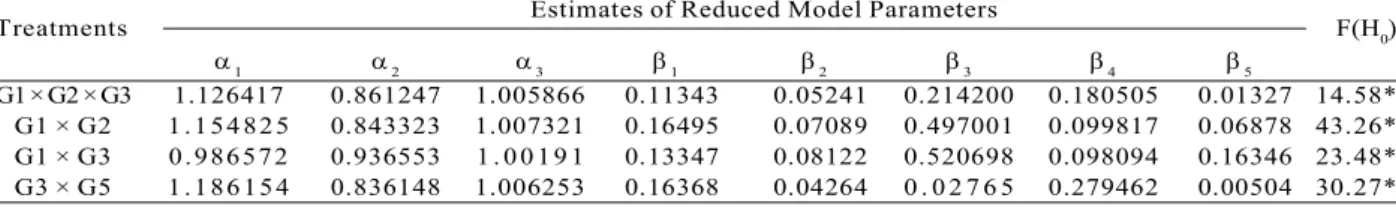
A model identity test was used to compare the stem profiles of the treatments estimated by Kozak (1988). Table 4 summarizes the comparison results. The effect of the genotype was observed among the treatments as shown in the resulting significant values.
The difference found in the stem form in all treatments suggests that a single model can be used in a management plan for wood assortments. However, the model parameters must be calculated for each treatment, i.e., for each genotype, a specific equation must be used.
4.DISCUSSION
The sigmoid model of Garay (1979) has shown satisfactory results, although not the best performance, for modeling tree stems of eucalyptus, Pinus, and teak plantations (Nogueira et al., 2008; Leite et al., 2011; Campos et al., 2014; Andrade, 2014). The sigmoid model of Biging (1984) was also highlighted in stem taper studies as shown in Soares et al. (2011) for natural forests in Brazil. The successful performances of sigmoid equations are attributed to their derivation from biological growth models, where the proposed taper equations attempt to establish the same relation on trunk narrowing from ground to the tree top.
Figure 1 – Distribution of residues of diameter estimates (cm) as a function of the observed diameters, and cases percentage per residue classes of the estimated diameter for models of Garay (1979), Kozak (1988), Max and Burkhart (1976), and Demaerschalk (1972).
Figura 1– Distribuição dos resíduos das estimativas de diâmetro, em cm, em função do diâmetro observado, e, percentagem
(Weiskittell et al., 2011). The generation of accurate volume estimates was insufficient to achieve satisfactory performance in describing the stem profile of the trees. Nevertheless, Môra et al. (2014) used this compatible model to yield estimates with a low bias for eucalyptus trees aged 8 years.
The segmented model of Max and Burkhart (1976) outperformed the variable exponent model of Kozak
(1988) in some sections of the stem. The performance of the segmented model for diameter estimates was not the most accurate, but showed better results than the sigmoid and compatible models. Except for the variable exponent model of Kozak (1988), the segmented model of Max and Burkhart (1976) showed lower dispersion of errors. Andrade et al. (2014) and Muhairwe (1999) also confirmed in comparison with the exponential and
Table 4 – Parameter estimates of Kozak (1988) taper model for comparison of model equality of the genotypes and F value for the identity test.
Tabela 4 – Estimativas dos parâmetros do modelo de Kozak (1988), para comparação da igualdade de tratamentos e correspondente
estatística F do teste de identidade.
Treatments Estimates of Reduced Model Parameters F(H0)
1 2 3 1 2 3 4 5
G1 × G2 × G3 1.126417 0.861247 1.005866 0.11343 0.05241 0.214200 0.180505 0.01327 14.58* G1 × G2 1.154825 0.843323 1.007321 0.16495 0.07089 0.497001 0.099817 0.06878 43.26* G1 × G3 0.986572 0.936553 1 . 00 19 1 0.13347 0.08122 0.520698 0.098094 0.16346 23.48* G3 × G5 1.186154 0.836148 1.006253 0.16368 0.04264 0 . 0 2 7 6 5 0.279462 0.00504 30.27*
*Significant at 5% probability.
Centro Garay Kozak Max and Demaerschalk
de Classe
n (1979) (1988) Burkhart (1976) 1972)
(DBH) Bias RMSE Bias RMSE Bias RMSE Bias RMSE
(%) (%) (%) (%) (%) (%) (%) (%)
G1:
1 12 0.647 7.292 0.308 7.617 0.682 7.577 0.310 8.539
2 12 0.841 7.976 0.801 7.943 0.807 7.807 1.390 8.929
3 12 1.103 7.539 0.492 6.924 1.137 7.091 0.933 7.891
4 15 0.267 7.735 0.020 6.098 0.231 6.586 0.007 7.993
5 12 1.648 7.570 1.601 5.799 1.687 5.588 1.6930 8.419
6 7 1.868 9.011 1.462 7.855 1.828 8.020 1.941 9.888
G2:
1 11 8.156 18.306 3.619 10.873 8.220 18.172 9.060 15.170
2 13 5.593 12.661 1.498 8.749 5.625 12.111 0.623 13.346
3 14 2.898 12.246 1.337 11.619 2.908 11.937 0.083 14.183
4 14 1.281 8.606 0.618 7.073 1.880 8.332 1.251 7.399
5 14 0.619 8.107 0.536 7.007 0.621 6.302 0.605 7.938
6 7 1.140 5.262 0.210 4.527 1.144 5.686 0.946 4.7470
G3:
1 12 8.661 14.138 1.021 9.108 8.671 14.100 1.612 10.311
2 11 8.019 11.649 2.482 8.391 8.001 11.769 2.677 9.093
3 16 1.583 9.321 0.796 8.286 1.558 8.802 1.389 12.167
4 13 0.483 10.442 0.417 9.570 0.405 9.118 0.381 9.520
5 13 0.228 9.044 0.095 7.271 0.266 7.189 0.120 7.482
6 7 2.479 9.420 0.706 8.518 2.527 9.497 0.048 9.054
Table 3 – Validation statistics for individual tree volume (m³ per tree) by diameter at breast height classes.
Tabela 3 – Estatísticas de Validação para a estimativa do volume total (m³ por árvore) para cada classe de DBH.
segmented models that despite the satisfactory performance of the segmented model of Max and Burkhart (1976), it did not present the best performance, which agrees with the results of the present work. Souza et al. (2008) tested some segmented models for eucalyptus trees and obtained the best results using the segmented model of Max and Burkhart (1976). Muhairwe (1999) confirmed that this model showed better results using data (sample trees) containing a low range of DBH and H, or even when the models were fitted by the diameter class. The segmented model of Max and Burkhart (1976) has the disadvantage of additional computational demands on simultaneous fitting of equations and the significant variation of the initial value of the parameters found in literature.
The exponential model of Kozak (1988), which is also called the variable exponent equation, showed great flexibility to describe the stem form of the genotypes, yielding accurate diameter and volume estimates. The successful performances of Kozak (1988) in predicting the diameters are attributed to the focus given by the author on the proposed equation, which assumptions are centered in modeling the tree bole. Kozak (1988) proposed a model whose restrictions determined a fixed inflection point and considers the geometric form variations along the stem, such as neiloid, paraboloid, and conic form. Similar to Andrade (2014), working with eucalyptus aged up to seven years, the performance of the estimates by Kozak (1988) was better than the compatible and sigmoid models. The good performance of this model could be associated with the size of the sample trees. The assumed inflection point (0.25 of the total height) was the assigned value chosen by the author of the equation in the original work for large trees in Canada. Modeling the stem taper of native eucalyptus trees in Australia, Muhairwe (1999) confirmed a better fit of the Kozak (1988) model to large trees in accordance with this study, and encourages the use of these equations for subsequent studies. Although the inflection point is fixed to eucalyptus and Pinus trees, this value may vary and should be changed for other tree species with previous estimation of the rate over the dataset.
The models of Max and Burkhart (1976) and Kozak (1988) showed the best performances for modeling the largest diameters, i.e., the diameter at the base region of the stem tree. Souza et al. (2008) elucidated that based on the occurrence of the greatest deformation of the stem in a tree with an abrupt change of geometric form, a consequent variation in the stem diameter values occurs. Bias related to small values of diameter estimates
can be tolerated because of its negligible effect on commercial volume calculus. However, when related to larger diameters, bias has an increasing effect and should be accounted for in cases where these diameters occur in relevant commercial sections (Figueiredo Filho et al., 1996).
Even if the parameters in Kozak (1988) were not restricted to generate a volume equation similar to the compatible models, the variable exponent model showed the most accurate individual tree volume estimates in this comparison. Goodwin (2009) in a study listing advantages and disadvantages of the taper models, points to the low ability of Kozak (1988) for modeling small trees of some species. Therefore, it is suggested that for the recognition of the variable exponent model as a reference to the stem taper of the eucalyptus trees, its accuracy on the estimate age classes can be evaluated, similar to Figueiredo Filho et al. (2015) for Araucaria angustifolia in southern Brazil.
5.CONCLUSION
The variable exponent model of Kozak (1988) was the model that fitted stem taper data in the most suitable manner, presenting the most accurate estimates for diameter and individual tree volume.
Based on Kozak (1988), it was possible to conclude that the genotype has a significant effect on the stem taper of eucalyptus trees, which must be considered when estimating the model parameters.
6.REFERENCES
Andrade VCL. Novos modelos de taper do tipo expoente-forma para descrever o perfil do fuste de árvores. Pesquisa Florestal Brasileira.
2014;34(80):1-13.
Biging, G. S. Taper equations for second mixed-conifers of Northern California. Forest Science, 1984;30(4):1103 17.
Campos BPF, Binoti DHB, Silva ML, Leite HG, Binoti MLMS. Efeito do modelo de afilamento utilizado sobre a conversão de fustes de árvores em multiprodutos. Scientia Forestalis.
2014;42(104):513-20.
Campos JCC, Ribeiro JC. Avaliação de dois modelos de taper em árvores de Pinus patula. Revista Árvore. 1982;6(2):140 9.
Demaerschalk JP, Kozak A. The whole-bole system: a conditional dual equation system for precise prediction of tree profiles. Canadian Journal for Research. 1977;7:488 97.
Demaerschalk JP. Converting volume equations to compatible taper equations. Forest Science, 1972;18(3):241-5.
Figueiredo Filho A, Borders BE, Hitch KL. Taper equations for Pinus taeda plantations in southern Brazil. Forest Ecology and Management.
1996;83:36-46.
Figueiredo Filho A, Restslaff FAZ, Kohler SV, Becker M, Brandes D. Efeito da idade no afilamento e sortimento em povoamentos de
Araucaria angustifolia. Floresta e Ambiente, 2015;22(1):50 9.
Garay L. Tropical forest utilization system. VIII A taper model for the entire stem profile, including buttressing. Seattle: Coll. Forest Res., Inst. Forest Prod. Univ. Wash., 1979. 64p. (Contribuition, 36).
Garcia SRL, Leite HG, Yared JAG Análise do perfil do tronco de Morototó (Didymopanax
morototonü) em função do espaçamento. In: Anais do 7º Congresso Florestal Brasileiro, 1º., Congresso Florestal Panamericano. Curitiba. Curitiba: SBS/SBEF; 1993. v.2. p.504-9.
Goodwin A N. A cubic tree taper model. Australian Forestry. 2009;72:8798.
Guimarães DP, Leite HG. Um novo modelo para descrever o perfil do tronco. Revista Árvore. 16(2):170-80.
Höjer AG. Tallers och granenes tillraxt. Stocklan: Biran till Fr. Loven. Om vara barrskorar; 1903.
Husch B, Miller CI, Beers TW. Forest
mensuration. 3rd. ed. Malabar: Krieger Publishing Company; 1993.
Islam N, Kurttila M, Mehtatalo L, Haara A. Analyzing the effects of inventory errors on holding-level forest plans: the case of
measurement error in the basal area of the dominated tree species. Silva Fennica. 2009;43(1):71-85.
Kozak A. My Last words on taper equations. Forestry Chronicle. 2004;80:507-14.
Kozak A. A variable exponent taper equation. Canadian Journal of Forest Research.
1988;18:1363 8.
Kozak A, Munro DD, Smith JHG. Taper functions and their applications in forest inventory. Forestry Chronicle. 1969;45(4):278 83.
Leite HG, Oliveira-Neto RR, Monte MA, Fardin L, Alcantara AM, Binoti MLMS. et al. Modelo de afilamento de cerne de Tectona grandis L.f. Scientia Forestalis. 2011;39(89):53 9.
Lima FS. Análise de funções “taper” destinadas à avaliação de multiprodutos de árvores de Pinus elliottii [dissertação] Viçosa, MG: Universidade Federal de Viçosa; 1986.
Max TA, Burkhart HE. Segmented polynomial regression applied to taper equations. Forest Science, 1976;22(33):283 9.
Môra R, Silva GF, Gonçalves FG, Soares CPB, Chichorro JF, Curto RDA. Análise de diferentes formas de ajuste de funções de afilamento. Scientia Forestalis. 2014;42(102):237-49.
Morley T, Little K. Comparison of taper functions between two planted and coppiced eucalypt clonal hybrids, South Africa. New Forests. 2012;43:129-41.
Muhairwe CK. Taper equations for Eucalyptus pilularis and Eucalyptus grandis for the north coast in New South Wales. Forest Ecology and Management. 1999;113:251-69.
Nogueira GS, Leite HG, Reis GG, Moreira AM. Influência do espaçamento inicial sobre a forma do fuste de árvores de Pinus taeda L. Revista Árvore. 2008;32(5):855 60.
Pereira JES, Ansuj AP, Muller I, Amador JP. Modelagem de volume de Eucalyptus grandis Hill ex Maiden. In: 12º Simpósio SIMPEP de
Engenharia de Produção. Bauru: 2005. Acesso em: 10 out. 2017. Disponível em: http://
www.simpep.feb.unesp.br/anais/anais_12/
copiar.php?arquivo=PEREIRA_JES_MODELO.pdf...
Regazzi AJ, Silva CHO. Teste para verificar a igualdade de parâmetros e a identidade de modelos de regressão não linear. I. Dados no delineamento inteiramente casualizado. Revista de Matemática e Estatística. 2004;22:33 45.
Schneider PR, Finger CAG, Klein JEM, Totti JÁ, Bazzo JL. Forma de tronco e sortimentos de madeira de Eucalyptus grandis Maiden para o estado do Rio Grande do Sul. Ciência Florestal. 1996;6(1):79 88.
Silva JA. Seleção de parcelas amostrais aplicadas em povoamentos de Pinus taeda L. para fins biométricos em Santa Maria – RS [dissertação] Santa Maria: Universidade Federal de Viçosa; 1974.
Soares CPB, Martins FBM, Leite Júnior HU, Silva GF, Figueiredo LTM. Equações hipsométricas, volumétricas e de taper para onze espécies nativas. Revista Árvore. 2011;35(5):1039 51.
Souza CAM, Silva GF, Xavier AC, Chichorro JF, Soares CPB, Souza AL. Avaliação de modelos de afilamento não-segmentados na estimação da altura e volume comercial de fustes de
Eucalyptus sp. Revista Ciência Florestal. 2008;18(3):393 405.