Computer Notes
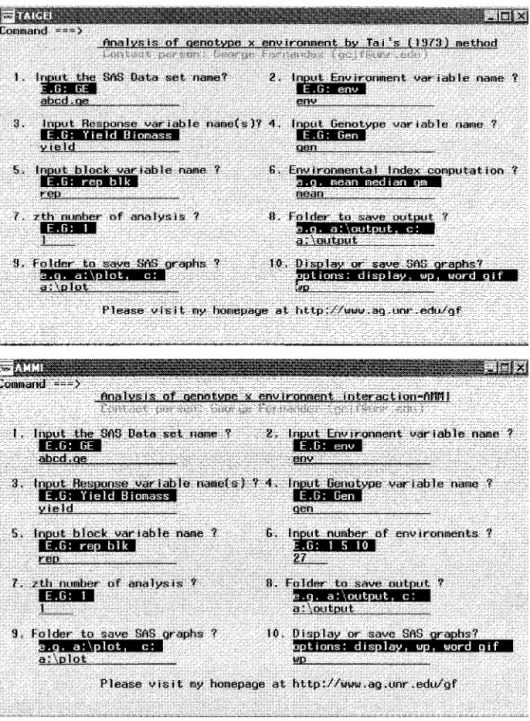
Figure 1. Screen shots of(a)TAIGEI and(b)AMMI MACRO-CALL windows.
SAS Applications for Tai’s
Stability Analysis and AMMI
Model in Genotype
ⴛ
Environmental Interaction
(GEI) Effects
M. Thillainathan and G. C. J.
Fernandez
A user-friendly graphical data analysis to perform stability analysis of genotype ⫻ environmental interactions, using Tai’s sta-bility model and additive main effects and multiplicative interaction (AMMI) biplots, are presented here. This practical ap-proach integrates statistical and graphical analysis tools available in SAS systems and provides user-friendly applications to perform complete stability analyses with-out writing SAS program statements or us-ing pull-down menu interfaces by runnus-ing the SAS macros in the background. By us-ing this macro approach, the agronomists and plant breeders can effectively perform stability analysis and spend more time in data exploration, interpretation of graphs, and output, rather than debugging their program errors. The necessary MACRO-CALL files can be downloaded from the author’s home page at http://www.ag.unr. edu/gf. The nature and the distinctive fea-tures of the graphics produced by these applications are illustrated by using pub-lished data.
Selection of genotypes for wide adaptabil-ity could be severely limited in the pres-ence of genotype⫻ environment
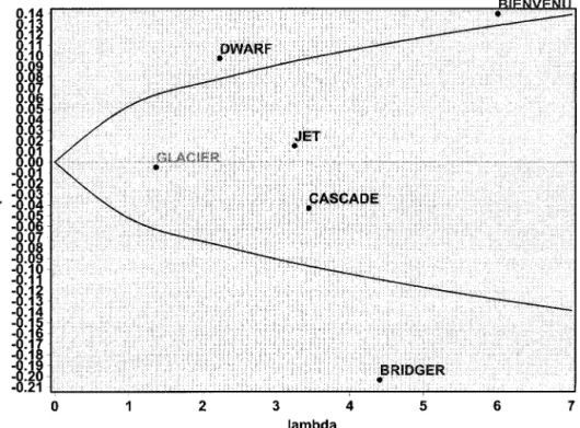
Figure 2. Tai’s (1971) stability plot showing different stability regions based on␣andstatistics. The hyper-bola represents a 95% prediction interval for␣ ⫽0; The vertical lines are the limits of a 95% confidence interval for ⫽1.
is measured by a statistic ␣, and the
de-viation from the linear response, which is measured by another statistic . A
per-fectly stable variety has (␣, ) ⫽ (⫺1,1)
and a variety with average stability is ex-pected to have (␣,)⫽(0,1). Tai’s
analy-sis also provides a method of obtaining the prediction interval for ␣ ⫽ 0 and a
confidence interval for values, so that
the genotypes can be distributed graphi-cally in different stability regions of the Tai’s plot.
The AMMI model is a hybrid analysis that incorporates both the additive and multiplicative components of the two-way data structure (Shafii et al. 1992; Shafii and Price 1998). The AMMI biplot analysis is considered to be an effective tool to di-agnose the GEI patterns graphically. In AMMI, the additive portion is separated from interaction by analysis of variance (ANOVA). Then the principal components analysis (PCA), which provides a multipli-cative model (Gabriel 1971; Zobel et al. 1988), is applied to analyze the interaction effect from the additive ANOVA model. The biplot display of PCA scores plotted against each other provides visual inspec-tion and interpretainspec-tion of the GEI compo-nents. Integrating biplot display and ge-notypic stability statistics enables geno-types to be grouped based on the
similar-ity of performance across diverse environ-ments.
Although many have published program codes for GEI studies in the past, these programs are not very user friendly. SAS program statements for performing Tai’s stability analysis were published previous-ly ( Fernandez 1991). SAS program state-ments to perform the AMMI analysis have also been presented (Shafii and Price 1998). However, the SAS program-based approach is considered difficult and not user friendly to agronomists, since a good programming knowledge in SAS is essen-tial to modify these published codes and to perform the GEI analyses. Therefore we have developed user-friendly SAS applica-tions to perform improved Tai’s stability analysis and AMMI models to analyze the GEI data.
Methodology
SAS version 6.12 for PC Win/NT was used to develop SAS MACRO programs and the relevant MACRO-CALL windows for Tai and AMMI analyses. The requirements for using these SAS macros are (1) a valid li-cense to run the SAS software on your PC, and (2) SAS modules such as SAS/BASE, SAS/STAT, SAS/GRAPH, and SAS/QC should
be installed in your computer to get the complete results.
The procedures for performing the user-friendly SAS macros are the following:
Tai’s Stability Analysis
Step 1.Create a GEI SAS dataset or down-load the sample dataset (Shafii and Price 1998) from the home page at http:// www.ag.unr.edu/gf. This data should con-tain the following variables:
Genotype variable (GEN), which is a categorical variable.
Environment variable ( ENV), which is a categorical variable.
Blocks or replications ( BLK); replica-tion will be treated as blocks.
Response variableY(e.g., yield), which is a continues numeric variable.
Step 2. Visit the home page ( Fernandez 2000) at http://www.ag.unr.edu/gf, click the running dog, and follow the instruc-tions given on the page to go to the down-load page. Then downdown-load Tai’s SAS MAC-RO-CALL window file by clicking the sample demo link, and save this file to a disk and open it in the SAS session. Finally, click the run icon to open the TAIGEI MAC-RO-CALL window ( Figure 1a).
Step 3. Input the required values by fol-lowing the instructions provided in the SAS MACRO-CALL window in TAIGEI ( Fig-ure 1a). In addition to inputting the SAS dataset name, environment variable name, response variable name, genotype vari-able name, and block varivari-able name in the MACRO-CALL window, the users are given the following options:
(1) Options for computing environmen-tal index, which is a quantitative measure of the environmental potential.
(a) mean:The environmental index for a given environment (EIj ⫽ the
arith-metic mean responses of all geno-types in the jth environment—the grand mean).
( b)median:The environmental index for a given environment (EIj⫽median
re-sponse of all genotypes in thejth en-vironment—median responses of all genotypes in all environments). This EI measure is recommenced when a few genotypes perform extremely low or high in some environments. (c) geometric mean (GM): The
environ-mental index for a given environment (EIj ⫽ the geometric mean response
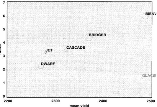
Figure 3. Relationships between Tai’s␣andstatistics and the genotypic mean response. The magnitude of the ␣statistic is proportional to the diameter of the bubbles in the plot.
Figure 4. Three-dimensional plot for Tai’s␣andstatistics versus the genotypic mean response. Different stability regions are denoted by different symbols.
means). This EI measure is recom-mended when most genotypes per-form extremely low or high in some environments.
(2) Options for saving the SAS output and SAS graphics files. Users can select the folders to save the SAS output and the graphics files by inputting the folder names in the MACRO-CALL window. Also, the users can select one of the following graphic file format when saving the graph-ics produced by the SAS macro:
Display: Files are not saved, but displayed in the SAS graphics Window.
WP: CGM files suitable for including in Corel Word Perfect products.
WORD: CGM files suitable for including in Microsoft products.
GIF: GIF files suitable for including in HTML-based Web documents.
Step 4. Submit the SAS macro. After in-putting all required fields, move your cur-sor to the last macro field, 10 ( Figure 1a), and hit the Enter key to run the SAS mac-ro. The MACRO-CALL window file auto-matically accesses the appropriate SAS macros from the Internet server, College of Agriculture, University of Nevada, and pro-vide the users with the required explora-tory graphs, stability estimates, and sta-bility plots.
AMMI Analysis
Step 1.Create a GEI SAS dataset or down-load the sample dataset from the home page ( Fernandez 2000) at http://www.ag. unr.edu/gf. This data should contain the same variables, listed above for running the Tai’s stability analysis.
Step 2. Visit the home page ( Fernandez 2000) at http://www.ag.unr.edu/gf, click the running dog, and follow the instruc-tions given to go to the download page. Download the AMMI SAS MACRO-CALL window file by clicking the sample demo link, save this file to a disk, and open it in the SAS session. Click the run icon to open the AMMI MACRO-CALL window ( Figure 1b).
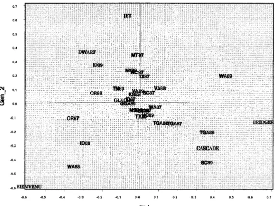
Figure 5. Biplot display of AMMI analysis for PCA component 2 versus PCA component 1 for six genotypes evaluated in 27 environments.
Figure 6. Biplot display of AMMI analysis for PCA component 1 versus mean responses for six genotypes eval-uated in 27 environments.
Step 4.Submit the SAS MACRO. Follow the instructions provided in Tai’s analysis.
Results and Discussion
By running these SAS macros, the users can obtain the following descriptive graphics illustrating the nature of GEI.
Tai’s Analysis
Figure 2 illustrates Tai’s stability plot based on␣andstatistics, which is
sim-ilar to the published figure (Shafii and Price 1998). It can be argued that the ␣
andstatistics derived from the GEI
com-ponent values are not sufficient to select the higher-yielding and stable genotypes, therefore the mean yield values also must be considered when making the decision. The lack of information about the average response is a shortcoming in Tai’s stability plot. To overcome this limitation we have included two additional plots, which in-clude average response value and Tai’s stability statistics in the same plot. The re-lationship between the mean response and values for each genotype is
illus-trated in a scatter plot ( Figure 3). The 95% confidence region for thestatistic is
il-lustrated as two horizontal lines. The di-ameter of the circle in the scatter plot is proportional to Tai’s ␣ statistic. A
three-dimensional plot of response mean versus Tai’s stability estimates (␣and) is shown
in Figure 4. This three-dimensional plot is useful to visually evaluate the yield poten-tial and stability estimates of the geno-types. The different symbols used in the three-dimensional plot separate the geno-types based on the statistical significance of Tai’s stability statistics.
AMMI Analysis
Two AMMI analysis biplots shown in Fig-ures 5 and 6 were obtained by running SAS macro for AMMI analysis, and these two biplots are similar to the published figures (Shafii and Price 1998). In the first biplot ( Figure 5), the first and second principal component (PCA1 and PCA2) scores for the genotypes and environments are dis-played. In the second biplot, the first PCA scores and the mean yields for genotype and the environments are displayed.
Conclusion
The availability of free and user-friendly SAS statistical and graphical applications to analyze GEI, based on Tai’s stability analysis and AMMI biplot analysis, are re-ported here. The steps involved in
down-loading the necessary MACRO-CALL files from the author’s home page ( http:// www.ag.unr.edu/gf ) and the instructions for running the SAS macros are presented
Table 1. Common data file formats used in DAMBE
Sequence format Read in Convert to
PHYLIP ⫹ ⫹
PAUP ⫹ ⫹
MEGA ⫹ ⫹
CLUSTAL ⫹ –
FASTA ⫹ ⫹
GenBank ⫹ ⫹
GCG ⫹ ⫹
MSF ⫹ ⫹
DNA strider ⫹ ⫹
PAML ⫹ ⫹
RST,MPa ⫹ –
PHYLTEST ⫺ ⫹
IG/Stanford ⫹ ⫹
NBRF ⫹ ⫹
EMBL ⫹ ⫹
FITCH ⫹ ⫹
PIR/CODATA ⫹ ⫹
Plain textb ⫹ ⫹
Allele frequency ⫹ –
Distance matrix ⫹ ⫹
aSequence formats for storing original sequences and
reconstructed ancestral sequences from the original sequences.
bThe one-sequence-per-file text format from programs
such as Sequence Navigator and DNA Star. From the Department of Applied Economics and
Statis-tics 204, University of Nevada, Reno, NV 89557. Ad-dress correspondence to George C. J. Fernandez at the address above.
䉷2001 The American Genetic Association
References
Gabriel KR, 1971. The biplot graphic display of matri-ces with application to principal component analysis. Biometrika 58:453–467.
Fernandez GCJ, 1991. Analysis of genotype⫻ environ-ment interaction by stability estimates. HortScience 26: 947–950.
Fernandez GCJ, 2000. Quick results from statistical analysis (visited/last modified August 16, 2000). http://www.ag.unr.edu/gf.
Shafii B, Mahler KA, Price WJ, and Auld DL, 1992. Ge-notype by environment interaction effects on winter rapeseed yield and oil content. Crop Sci 32:922–927.
Shafii B and Price WJ, 1998. Analysis of genotype-by-environment interaction using the additive main effects and multiplicative interaction model and stability esti-mates. J Agric Biol Environ Stat 3:335–345. http:// www.uidaho.edu/ag/statprog/ammi/.
Tai GCC, 1971. Genotypic stability analysis and its ap-plication to potato regional trials. Crop Sci 11:184–190.
Zobel RW, Wright MJ, and Gauch HG, 1988. Statistical analysis of a yield trial. Agron J 80:388–393.
Received September 7, 2000 Accepted April 30, 2001
Corresponding Editor: Bruce S. Weir
DAMBE: Software Package
for Data Analysis in
Molecular Biology and
Evolution
X. Xia and Z. Xie
DAMBE (data analysis in molecular biolo-gy and evolution) is an integrated software package for converting, manipulating, sta-tistically and graphically describing, and analyzing molecular sequence data with a user-friendly Windows 95/98/2000/NT in-terface. DAMBE is free and can be down-loaded from http://web.hku.hk/⬃xxia/ software/software.htm. The current version is 4.0.36.
DAMBE (data analysis in molecular biolo-gy and evolution) is an integrated puter program for descriptive and com-parative analysis of molecular data (including nucleotide and amino acid se-quence data, as well as allele frequency and distance matrix data). It has features either not available or poorly implement-ed in other programs. These features are grouped into (1) sequence format conver-sion and manipulation supporting 20 com-monly used molecular data formats; (2)
descriptive statistics such as nucleotide, amino acid, and codon frequencies, dinu-cleotide and diamino acid frequencies, analysis of codon usage and amino acid usage bias; and (3) comparative sequence analysis such as phylogenetic reconstruc-tion of trees and ancestral sequences with distance, maximum parsimony and maxi-mum-likelihood methods, bootstrapping and jackknifing, significance tests of mo-lecular clock and alternative phylogenetic hypotheses (i.e., how much better is the best tree compared to alternative trees), fitting statistical distributions to substitu-tion data over sites including Poisson, negative binomial, and gamma distribu-tions. DAMBE features a user-friendly Win-dows interface with extensive on-line help.
Sequence Input and Sequence
Format Conversion
DAMBE can read and convert almost all commonly used molecular data formats ( Table 1). In particular, DAMBE can take advantage of the rich information con-tained in the FEATURES table of GenBank files and extract specific segments such as CDS, exons, introns, rRNA, etc., by a few mouse clicks. The user can also use ‘‘cus-tom splicing’’ to extract sequence seg-ments that are not specified in the Gen-Bank sequences.
DAMBE can read sequence files directly from a networked computer, such as a re-mote UNIX workstation, in the same way as one would read a file from a local hard
disk. Extensive network functions have also been implemented for retrieving se-quences directly from GenBank, either by LOCUS name or accession number, or by keyword search.
DAMBE features a color-coded se-quence editor for either sese-quence input or visual alignment. Sequences can be as long as 32,768 bp.
Sequence Manipulation
We will only highlight two of the many se-quence manipulation features in DAMBE.
Sequence Alignment
DAMBE can align nucleotide and amino acid sequences as most other alignment programs do. However, one particular fea-ture that is not available in most other alignment programs is the ability to align protein-coding nucleotide sequences against aligned amino acid sequences. Other programs often introduce frame-shift indels in the aligned protein-coding sequences, even if the protein genes are known to be functional and do not have these frame-shifting indels. In other words, the introduced frame-shifting indels in the aligned sequences are alignment artifacts, and the correctly aligned sequences should have complete codons, not one or two nucleotides, inserted or deleted.
DAMBE solves this problem by aligning the protein-coding nucleotide sequences against aligned amino acid sequences. One can read in the protein-coding nucle-otide sequences, translate them into ami-no acid sequences, align the amiami-no acid sequences, and then align the original nu-cleotide sequences against the aligned amino acid sequences.
Translation
DAMBE implements all 12 different genetic codes and can therefore translate protein-coding nucleotide sequences from any or-ganism to amino acid sequences. The im-plementation of these genetic codes greatly facilitates amino acid-based and codon-based analyses.
Descriptive Sequence Analysis
This includes nucleotide, amino acid and codon usage analysis, compositional anal-ysis based on dinucleotide and diamino acid frequencies, quantification of the ef-fect of GC and TpA frequencies on exon
and CDS lengths, and the methylation ef-fect on codon usage bias.