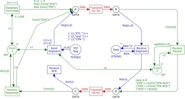
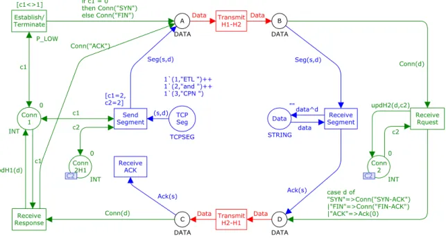
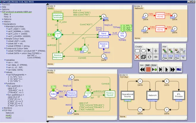
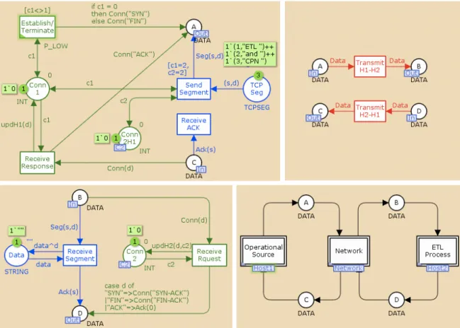
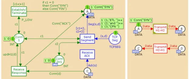
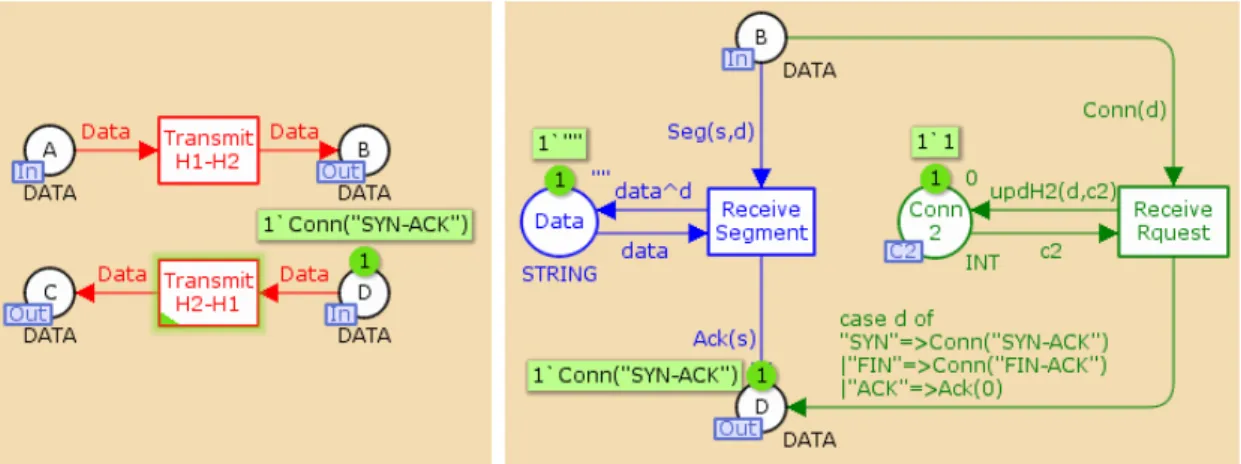
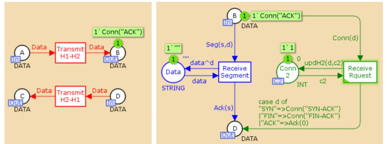
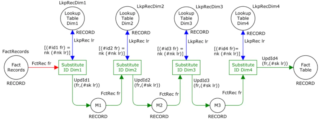
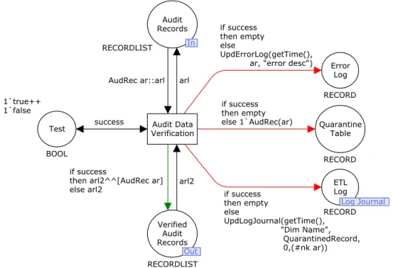
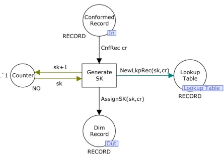
ETL systems modelling with Coloured Petri Nets

We find a correlation between the structural indicators and the number of member, structure, independence and experience of the members of the Audit Committee. The audit

The structure of the remelting zone of the steel C90 steel be- fore conventional tempering consitute cells, dendritic cells, sur- rounded with the cementite, inside of

Since this is an international issue as it involves rights recognized under international agreements (UDHR, ICESCR, TRIPS), actors from different States (Novartis,

Artur, sócio da personagem-narrador, não dá importância ao fato, posto que seja considerado normal; João Mudo, sujeito mudo e surto, mantém-se indiferente; Coló,

Na expectativa de conscientizar os alunos acerca do que vai ser estudado para que eles se envolvam com a matéria e com isso despertem o interesse por novas experiências,

A pesquisa tem como principais objetivos: contribuir para o desenvolvimento dos estudos aplicados da administração, gestão da comunicação e psicologia organizacional, assim

As teses e dissertações encontradas foram agrupadas em 27 categorias temáticas sendo elas: Alfabetização, Aprendizagem Colaborativa, Artefatos Pedagógicos,

It is the leading journal contributing with 16 themes in auditing (Table 3), of which are prominent: audit market (MRKT), audit procedures (PROC), audit report & fi