Universidade do Minho Escola de Engenharia Departamento de Inform´atica
Joao Paulo Fontoura Moutinho Magalhaes
Power aware scheduler
for heterogeneous environments
Universidade do Minho Escola de Engenharia Departamento de Inform´atica
Joao Paulo Fontoura Moutinho Magalhaes
Power aware scheduler
for heterogeneous environments
Master dissertation
Master Degree in Computer Science
Dissertation supervised by
Alberto Jose G. de C. Proenca Joao Garcia Barbosa
A C K N O W L E D G E M E N T S
First and foremost I would like to thank my mother, the person that has always been there for me and without whom none of this would be possible.
I want to thank both my advisors Alberto Proenc¸a and Jo˜ao Barbosa for all the help they gave me and for the opportunities they have provided.
I also want to thank my family for supporting me when times were hardest, especially my sister for putting up with me all of this time.
Last but not least I would like to thank my friends for all the good times and especially thank C´elia Ferreira, John Maia and Jos´e Luis Silva for helping me on some parts of this thesis.
A B S T R A C T
Efficient or green computing is becoming a key issue in current programming techniques, going beyond high performance computing, by simultaneously considering issues such as energy or power consumption. In heterogeneous environments, where different processors and accelerators co-processors may coexist, there is a real opportunity to reduce the overall energy consumption of the system by using scheduling decisions in run-time that can have a good and quick response to changes in the different components.
Current tools to aid the development of efficient applications lack yet these run-time facil-ities. This motivated the development of a new framework with a power-aware scheduler for heterogeneous environments, PASH-Frame, whose prototype is the key object of this dissertation. This work extended previous performance-based scheduling work to include run-time power-aware features, adding tools to measure power consumption at each device and using different scheduling decisions to get the best outcome according to pre-defined targets by the end user.
To evaluate the overall behaviour of PASH-Frame, several tests were performed: 1000 SAXPY tasks with vector sizes varying from 16 thousand elements to 256 thousand; 200 SGEMM tasks with matrices varying from 64 thousand elements to 16 million and finally a test that combines the two previous ones. Results show that the scheduling algorithm implemented in the framework can achieve good results in some cases, in spite of not being able to make some critical decisions when it comes to energy consumption reduction like forcing a component to idle to save energy.
R E S U M O
Computac¸˜ao eficiente (ou green computing) est´a a tornar-se um dos maiores desafios nas t´ecnicas de programac¸˜ao actuais, considerando simultˆaneamente os problemas de computac¸˜ao de alta performance bem como a energia e o consumo total. Em ambientes heterog´eneos, onde diferentes processadores e aceleradores como co-processadores podem coexistir, ex-iste uma grande oportunidade para reduzir o consumo energ´etico global do sex-istema ao utilizar decis ˜oes de escalonamento em tempo real que conseguem ter uma boa resposta r´apida a mudanc¸as nos diferentes componentes.
As ferramentas actuais para ajudar na programac¸˜ao de aplicac¸ ˜oes eficientes ainda n˜ao tˆem estas ferramentas de leitura de energia em tempo real. Isto serviu de motivac¸˜ao para criar uma nova framework com um escalonador para sistemas heterog´eneos consiente do gasto de energia, a PASH-Frame, em que o seu prot ´otipo vai ser explicado nesta dissertac¸˜ao. Este trabalho ´e uma continuac¸˜ao de trabalho pr´evio em escalonamento baseado em alta performance ao incluir ferramentas de medic¸˜ao de energia em tempo real e ao fornecer de-cis ˜oes de escalonamento baseadas nesses valores para ter o melhor desempenho de acordo com as escolhas do seu utilizador.
Para avaliar o comportamento da PASH-Frame, varios testes foram feitos: o primeiro teste foi de 1000 tarefas do algoritmo SAXPY com o tamanho dos vetores a variar entre 16 mil elementos e 256 mil; o segundo teste foi de 200 tarefas do algoritmo SGEMM com os tamanhos das matrizes a variar entre 64 mil elementos e 16 milh ˜oes de elementos e por fim o terceiro teste ´e uma combinac¸˜ao dos dois primeiros. Os resultados obtidos mostram que o algoritmo de escalonamento implementado na framework consegue obter bons resultados em alguns casos, apesar de n˜ao conseguir fazer algumas decis ˜oes cr´ıticas para o escalon-amento com vista a reduzir o consumo global do sistema, como forc¸ar um componente a ficar inativo para poupar energia.
C O N T E N T S
1 i n t r o d u c t i o n 1
1.1 Context 1
1.2 Goals, Motivation, Contribution 2
1.3 Overview 3
2 s c h e d u l i n g 4
2.1 Challenges of scheduling on an heterogeneous environment 5
2.2 Scheduling oriented to performance 6
2.2.1 A simple simulator for load balancing 8
2.3 Measuring power consumption in devices 9
2.4 Power-aware scheduling 11
2.5 Performance vs. Power-aware: a SWOT analysis 14
3 pa s h-frame, an efficient scheduling tool 17
3.1 The scheduler model 17
3.1.1 Scheduling decisions 21
3.2 Scheduling tuning 24
3.3 The support framework 24
4 t e s t a n d e va l uat i o n 28
4.1 Testbed 29
4.2 Discussion of results 30
5 c o n c l u s i o n s 41
5.1 Suggestions for future work 41
a l i s t o f s c h e d u l i n g d e c i s i o n s a na ly s e d a n d r e s p e c t i v e pa p e r s 45
L I S T O F F I G U R E S
Figure 1 DAG example 5
Figure 2 Explanation of what combinations are on this scheduler 20
Figure 3 Consumption calculation with instant consumption readings 21
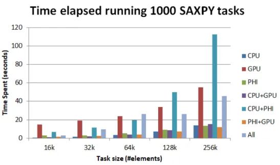
Figure 4 Total time spent running 1000 SAXPY tasks with different worker combinations and task sizes 31
Figure 5 Energy consumption while running 1000 SAXPY tasks with different worker combinations and task sizes 32
Figure 6 Wait percentage of CPU-GPU combination for SAXPY tasks with 16k
element vectors 32
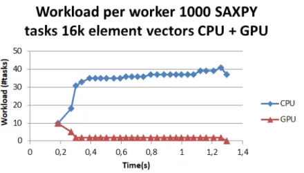
Figure 7 Workload distribution of CPU-GPU combination for SAXPY tasks
with 16k element vectors 33
Figure 8 Wait percentage of PHI-GPU combination for SAXPY tasks with 256k
element vectors 33
Figure 9 Workload distribution of PHI-GPU combination for SAXPY tasks
with 256k element vectors 34
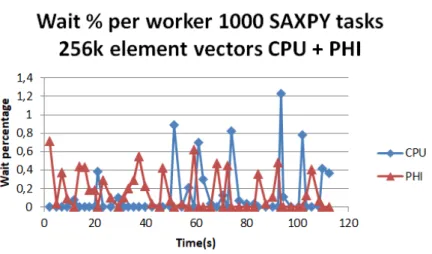
Figure 10 Wait percentage of CPU-PHI combination for SAXPY tasks with 256k
element vectors 34
Figure 11 Workload distribution of CPU-PHI combination for SAXPY tasks
with 256k element vectors 35
Figure 12 Wait percentage of All worker combination for SAXPY tasks with
256k element vectors 35
Figure 13 Workload distribution of All worker combination for SAXPY tasks
with 256k element vectors 36
Figure 14 Total time spent running 200 SGEMM tasks with different worker combinations and task sizes 37
Figure 15 Energy consumption while running 200 SGEMM tasks with different worker combinations and task sizes 38
Figure 16 Wait percentage of PHI-GPU combination for SGEMM tasks with
64k element matrices 38
Figure 17 Workload distribution of PHI-GPU combination for SGEMM tasks
with 64k element matrices 39
Figure 18 Wait percentage of PHI-GPU combination for SGEMM tasks with
16M element matrices 39
List of Figures vi Figure 19 Workload distribution of PHI-GPU combination for SGEMM tasks
with 16M element matrices 39
Figure 20 Total time spent running 1000 SAXPY tasks and 200 SGEMM tasks with different worker combinations and task sizes 40
Figure 21 Energy consumption while running 1000 SAXPY tasks and 200 SGEMM tasks with different worker combinations and task sizes 40
L I S T O F TA B L E S
Table 1 Relation table values for the scheduling decision combination
exam-ple 22
Table 2 Compute node configuration 29
Table 3 Configuration of the Stampede system 30
Table 4 Power consumption of each device and combined 30
Table 5 Power consumption of each device and combined 31
1
I N T R O D U C T I O N1.1 c o n t e x t
The usage of heterogeneous architectures is increasing inHigh Performance Computing (HPC). These heterogeneous architectures have coprocessors such asGraphical Processing Unit (GPU)s and the many core Intel Xeon Phi in addition to the multi-core processor to increase the computational power of the system and to specially increase the system performance when running particular tasks. Algorithms with a lot of parallelism such asSingle Instruction, Mul-tiple Data (SIMD)instructions are specially faster on coprocessors due to the high amount of parallelism in their architecture. Despite having a lot of advantages there are extra chal-lenges that arise when using an heterogeneous architecture. When using coprocessors the memory has to be transferred from the processor’s memory to the coprocessor’s which takes time and costs extra energy since the bus between the two needs to transfer the data. Since the coprocessors are better or worse than the processor depending on the tasks being ran, the work distribution among the processing components can also influence the perfor-mance of an application. For simplicity, all the various processing components (processors, coprocessors andGPUs) will be called devices in this report.
An emerging concern in computer science is green computing. Green computing stands for the study and practice of environmentally friendly techniques to lessen the impacts of the information technology, including the decrease in the usage of hazardous materials in manufacturing, the maximisation of energy efficiency and the reusability and recyclabil-ity of dying products and waste. Green computing is particularly critical and effective in two different areas: mobile devices and large systems (data centres, supercomputers, large companies with lots of servers or terminals, ...). On mobile devices, the main issue is the limited energy availability since batteries can not store infinite energy. Large systems are the main energy consumers in the information technology and, due to the huge amount of components, a small improvement on several components can make a huge difference in the energy bill. This concern in energy efficiency is specially noticeable in HPC where two types of challenges exist: who can create the fastest supercomputer and who can create
1.2. Goals, Motivation, Contribution 2
the most efficient / green supercomputer (the efficiency is measured inMega Floating-Point Operations Per Watt (MFLOP/W)). As of November 2016, three of the ten fastest supercom-puters in the world are also in the top ten of the most efficient ones with the fastest su-percomputer being in the fourth place in the top ten green susu-percomputer list. Because of this emerging concern in energy efficiency component manufacturers are trying to ease the measurement of energy consumption by creating measurements based on software instead of needing external devices, which allows the measurements to be made without the need for external devices that would make the energy measurement costly (both in time to read the data and in the amount of measuring devices needed to measure different components).
Since the majority of programmers are neither familiar with code optimisation (paral-lelization, vectorization, ...) nor the challenges that come with heterogeneous environments (programming for GPUs, workload distribution, ...) the usage of schedulers that help the user solving these problems is increasing. These schedulers overlay the Operating System (OS) scheduling to handle the workload distribution and are usually found as part of a framework that eases the user’s work by managing the memory of all the work automati-cally and even being able to optimise the code.
1.2 g oa l s, motivation, contribution
With some experience with schedulers (creating a simulator that can test scheduling func-tions and a scheduling function for balancing different task types in an heterogeneous environment), there is a great motivation for me to be a part of this project.
The goals of this project are the following:
• create samplers to measure the energy consumption of the different devices connected to the system without the need for external equipment;
• explore ways to use the energy measurements obtained from the samplers to schedule the work among the devices connected to the system;
• create a framework that enables the use of the samplers as well as the scheduler.
The main contribution of this work was the development of a framework prototype to aid the development of energy efficient applications on heterogeneous environments, by providing samplers to measure the energy consumption of each device in a compute server and containing alternative scheduler techniques that consider both the performance and energy consumption of each device in the overall solution)
1.3. Overview 3
1.3 ov e r v i e w
Section 2 explains the different problems of performance and power-centered schedulers on heterogeneous environments. Some of the schedulers currently used are revised, and compared between each other. Section 3 presents the PASH-Frame framework. Section 4 presents the tests done to the PASH-Frame framework and the results. Section 5 concludes this document and present suggestions for future work.
2
S C H E D U L I N GA scheduler is a method to assign work to computational resources based on the character-istics of the work itself and on its behaviour when being ran in each of the computational resources. Schedulers are used in a variety of ways: some can be used try to balance the workload given to each resource so as to minimise the idle time of the resources while other are used to allow multiple users to share access to system resources keeping the best
Quality of Service (QoS)possible.
Schedulers can be placed in two extreme positions of the software: as a part of the op-erating system or embedded in the application. There is also a solution in between: as an
Application Programming Interface (API) that schedules independent tasks across the avail-able resources, usually availavail-able within a development framework. This work follows this mid approach proposing and developing a prototype of a power-aware scheduler for het-erogeneous environments framework, the PASH-Frame. This framework is mainly a library of functions to aid the adequate scheduling of task-based programs on heterogeneous envi-ronments, aiming the following key goals: maximum performance with minimum energy consumption.
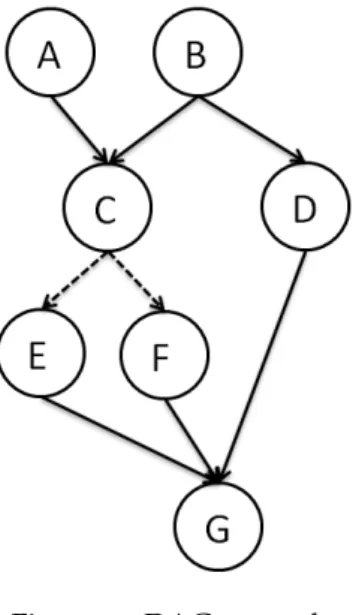
Scheduling of independent tasks favours task-based programming, which uses logical tasks instead of threads to formulate the program with some advantages, such as an easier load balancing among the computational devices and allowing opportunities to apply run-time parallelisation techniques. When using task-based programming with expressions, constructs and a set of conditional statements, a program can be represented as a Directed Acyclic Graph (DAG), where each code block is represented as a task and each dependency between code blocks is represented as a link between tasks.
Figure1shows a possible DAG for a simple program where the first tasks ran are A and
B with D starting only after B ends and C only able to start after A and B finish. While continuous links represent the data transfer needs of the tasks, the dotted lines represent logical conditions that can not be true at the same time. In Figure 1 tasks E and F are
connected to C through a logical condition so either task E or task F is executed, never both.
2.1. Challenges of scheduling on an heterogeneous environment 5
Since tasks E and F are mutually exclusive they can be assigned to the same time slot on a computational resource.
DAGs like the one presented in Figure1can be used not only to represent the work of a
big independent task divided into small, and usually dependent, tasks but also to express the relations between a large number of dependent tasks.
Figure 1.: DAG example
The next section presents some challenges of heterogeneous environments and the follow-ing sections cover the main issues related to a schedulfollow-ing framework: performance-based and power-aware.
2.1 c h a l l e n g e s o f s c h e d u l i n g o n a n h e t e r o g e n e o u s e n v i r o n m e n t
When scheduling for heterogeneous environments extra challenges arise. An heteroge-neous environment means that coprocessors (likeGPUs or the Intel Xeon Phi) are used in combination with the, usually multi-core,Central Processing Unit (CPU). These coprocessors are specially useful in particular tasks, depending on the architecture. In the case of most
GPUs and also the Intel Xeon Phi, the parallel oriented architecture makes these devices specially effective in algorithms with a great number of SIMD instructions, which are ap-plied to a range of data and can be ran at the same time. Vectorization can greatly improve the performance of a code by applying the same instructions to a range of different data within a vector instead of just doing a simple scalar operation. In the case of the Stream-ing SIMD Extensions (SSE) instruction set, it is possible to do four operations with single precision floating point values at the same time and with the Advanced Vector Extensions (AVX) extensions it is possible to do eight operations with single precision floating point
2.2. Scheduling oriented to performance 6
values at the same time, with a multiplication and addition able to be fused into a new operation calledFused Mutiply-Add (FMA). Vectorization is applied within a single core so a multi-coreCPUwith eight cores equipped with theAVXextension can be able to do 64 (8 cores * the 8 floating point operations done by each one) operations of the same type at the same time, as long as the memory is able to be loaded at the same time which obligates the programmer to think about the spatial locality (the data needed to be accessed is aligned continuously in memory, as a one-dimensional array for example) of the data. With the use of vectorization and coprocessors with a lot of processing elements the speedup of a code with a lot ofSIMDinstructions can be huge.
Despite the advantages of using heterogeneous environments there are challenges that appear which would not be a problem in an homogeneous environment. Since the co-processors are separated from the processor, their memory is also different from the main memory in the processor. To be able to transfer memory from the processor to the copro-cessor (or the other way around) a BUS between the two has to be used. Since coprocopro-cessors have a huge performance on some types of tasks the BUS connecting the coprocessor to the processor may not be able to handle the transfer of all the data needed to keep the copro-cessor running at maximum performance which causes a bottleneck. The memory transfer overhead can be masked by doing asynchronous communication, i.e. by decoupling the execution with the data transfer and transferring the data from the next task while running the current one.
Since the performance and the general behaviour of the coprocessors is different from the processor and depends on the type of task being computed, the workload balancing between various devices within the same system is critical to the overall performance. The problem of load balancing can not be easily resolved since it depends on the properties of both the tasks being ran and the devices running them.
2.2 s c h e d u l i n g o r i e n t e d t o p e r f o r m a n c e
When trying to obtain the best performance possible on heterogeneous systems, there are two types of scheduling that are equally important to the overall throughput of the system: inter and intra-device scheduling where the first refers to the scheduling of tasks between the devices available in the system and the latter refers to the scheduling of tasks within the same device.
2.2. Scheduling oriented to performance 7
Traditionally, the intra-device scheduling was done by the task programmer which needed to handle the load balancing between computational resources within the same device (for example handling the code each core runs within the same multi-coreCPU) as well as guar-antee that the data could be accessed in a way that vectorization was possible (by using one dimensional arrays with sequential accesses for example) and that the cache of the compu-tational resources was coherent throughout the device. APIs like OpenMP (OpenMP(2016))
can help the programmer parallelise the code by automatically distributing the work among the computational resources available within the device. Libraries like the Intel Math Ker-net Library (MKL)and the NVidia cuBLAS have highly optimised implementations of some standard tasks like GEMM or AXPY for various types of data like single or double precision floating point numbers for each of the device types (cuBLAS for CUDA capableGPUs and theMKLlibrary for the multi and many core Intel processors and coprocessors).
This dissertation is an extension of the work of Ribeiro et al. (2015), who developed a
performance-oriented framework to handle both regular and irregular applications on het-erogeneous systems. The framework presented in Ribeiro et al.(2015) has an inter-device
scheduler based on a demand driven approach where each device is able to request work from the global task queue (the same for every task ready to be computed).
The framework proposed inRibeiro et al.(2015) uses theHeterogeneous Earliest Finish Time (HEFT)technique, similar to the one used on StarPU. The data management system of the framework uses a MSI cache coherence protocol, also similar to the one used in StarPU, enabling data replication and ensuring consistency among replicas which is combined with a lazy data transfer policy to reduce the data movement overhead. It also supports data pre-fetching and the overlapping of asynchronous data transfers with computation. The main difference between the framework presented in Ribeiro et al. (2015) and the StarPU
framework is that the one presented in Ribeiro et al. (2015) has a different performance
model and a mechanism to partition the work in run-time.
The framework developed byRibeiro et al.(2015) can handle two types of kernels (tasks):
consumer and consumer-producer tasks. The first type represents a full task and is as-signed as a whole to a device. The parallelisation and optimisations made to the task itself are the responsibility of the task’s programmer. The second type of task represents theBasic Work Unit (BWU) of a task, i.e the operation that is done to a single piece of data during the task’s execution. This task is independent from all the BWU tasks (this independence must be assured by the task’s programmer) so it can also be assigned independently from the other BWUtasks of the same task so they can be ran together as a bundle on a device that supports vectorization. These tasks spawn new ones that perform the same BWUon
2.2. Scheduling oriented to performance 8
a different set of data. These new tasks are enqueued into the local outbox queue of the device and then enqueued into it’s local inbox queue if there is still room or into the global inbox queue if there is not enough space in the local inbox queue.
2.2.1 A simple simulator for load balancing
To test the scheduling model and the scheduling decisions a simple simulator was devel-oped in in a previous team work internship at University of Texas at Austin (co-author: John Maia), based on the work of Ribeiro et al.(2015). This tool is based on the consumer
tasks explained in section 2.2 and can simulate a set of pre-defined synthetic tasks (with
a sleep timer which is bigger or smaller depending on the attributes chosen by the user) running in a set of pre-defined computing devices, the workers.
The attributes for the two main entities (the tasks and the workers) of the simulation are introduced by the user in the source code. Attributes that pre-define each task behaviour include its weight, number of loads/stores, cost of branching and cache misses. Attributes that pre-define each worker behaviour include its latency, throughput, capacity, time to transfer tasks and costs of load/store/instruction executions. The outcomes of each simula-tion run include informasimula-tion about the workload balancing between workers, the behaviour of each worker during the run and the total time taken to complete all of the work.
This simulator works in iterations. An iteration starts when the scheduler assigns work to the workers and ends when all the workers complete the tasks assigned to them. In each iteration the scheduler assigns a task type to each worker based on what task type best fits the objective function of the scheduler, which in this case is the maximum perfor-mance possible. The load balancing step is different from the task type decision step in this simulator. Since the behaviour of each task type is different from worker to worker, the load balancing has to take into account which worker is running which type of task, this is called a combination (explained in section3.1).
The simulator starts with a small block of tasks and distributes them between the work-ers. When the combination is ran again, the information about how much time each worker waited for the others to finish their work on the last iteration is used to redistribute the block of tasks between the workers. When the distribution of the block of tasks between the workers is so stable that no worker waits more than a defined percentage of time and that stability endures through a number of iterations, the size of the block of tasks is
dou-2.3. Measuring power consumption in devices 9
bled maintaining the workload percentages of each worker.
This simulator can be modified to support accurate simulation of the behaviour of differ-ent tasks and workers in terms of both time and power consumption. This would require the addition of a technique to measure the power consumption of each type of instruction on each type of worker, similar to the ones presented inHao et al.(2013) andBrabrand et al.
(2012).
To measure the power consumption of the tasks in each worker, the simulator would need (i) to estimate the power consumption of each instruction type on each worker, (ii) to compute the number of instructions of each type on a given task and (iii) to estimate the idle consumption of the workers. Only then can the simulator be used to simulate tasks on that specific system.
Since these required power-aware modifications outweigh the simulator usefulness, it was decided not to use the simulator, opting by developing a framework that can use the power samplers created (see section2.3).
2.3 m e a s u r i n g p o w e r c o n s u m p t i o n i n d e v i c e s
Before the introduction of software power counter by device manufacturers, the energy measurement of a single devices or an entire systems would require external measuring equipment connected to the device or to the power supply. In cases where there is the need to measure N devices inside the same system, there would be the need to have at least N external measuring devices which is not only expensive but completely impossible when there are hundreds or maybe thousands of systems to be measured at the same time.
Before these power counters were introduced, design-time techniques for evaluation of time and power consumption were used, specially on Software Product Lines (SPL) appli-cations since most of the code is the same for two different appliappli-cations within the same
SPL. Hao et al. (2013) and Brabrand et al.(2012) use these kind of techniques to estimate
the power consumption of a code by measuring the power consumption of each basic in-struction and data transfer and estimating the total power consumption of a given code accordingly to the number of instructions of each type and the data of those instructions.
SPLs are specially good test cases for this type of estimations since, by testing code for a given application, the probability of another application within the same SPL having a large amount of equal code is very high. Accordingly to tests made inHao et al.(2013), the
2.3. Measuring power consumption in devices 10
tests made on a set of mobile applications of the Google Play store.
With the increase of concern regarding power consumption device manufacturers started to add software energy measuring tools. These tools can be found in most devices created now-a-days and vary depending on the manufacturer, the device type and even in the prod-uct’s family.
Intel multicore devices
In case of Intel processors, from the Sandy Bridge generation on, there is an interface that can calculate the energy consumption, by providing a software power model that uses hard-ware performance counters and I/O models, called Running Average Power Limit (RAPL).
RAPLprovides three different interfaces to access the accumulated consumption of the pro-cessor, in Joules. The RAPLinterface used for the power readers was the Machine-Specific Registry (MSR)counters (available on Linux under /dev/cpu/*/msr) since is the one with the least overhead. This counter can overflow, which is a problem that the reader has to handle. Because of the differences in the architecture, different generation processors have different overflow values. In spite of the low overhead theMSRcounters must be accessed with root privileges.
Intel many-core devices
In case of the Intel Xeon Phi power counters there are two different ways they can be accessed: using the CPU or the coprocessor itself. The information about the Xeon Phi consumption is measured using in the CPU by using the command ”micsmc -f ” which returns the current power consumption of the device, in Watts. Measurements through the device itself were not done but the values are available under ”/sys/class/micras/power”.
NVidia GPU devices
In NVIDIAGPUs there are two interfaces that can be used to measure the power consump-tion of the card. One of them is CUDA Profiling Tools Interface (CUPTI) that works based on events chosen by the user to return system counters which can sound great but has a terrible measurement rate (in tests made every measurement needed at least one second difference from another). The other interface is Nvidia Management Library (NVML)which is part of the NVIDIA Software Development Kit (SDK)and does not have a minimum time between measurements. Since theNVML’s interface level is lower level thanCUPTI’s, mea-surements made usingNVMLhave a much lower overhead.
2.4. Power-aware scheduling 11
With the use of these power readers, a library was developed to enable easy access to the time and energy cost of each piece of code. Using the developed library, the user only has to start the device’s power reader before running the code and stop it after finishing the code. The reader returns information like average power consumption, minimum and max-imum readings, and total power consumed and can also be reset with a simple function. It is possible to save the readings into a file, which is useful for analysing both performance and power consumption hotspots.
It is possible to use the power readers to help schedulers make decisions that decrease the overall consumption of the computation. Power readers can only measure the energy consumption of the device so, since the computational resources within the device can not be measured separately, the power readers are only useful for inter-device scheduling and are not fine-grained enough to be used on in intra-device scheduling yet.
2.4 p o w e r-aware scheduling
Power-centered scheduling focuses on minimising the energy consumption of the system when running the tasks. In addition to the scheduling goals of performance oriented sched-ulers, the power-centered schedulers also have to take into account the energy consumption of each task when running on each device and the energy consumption of transferring data from one computational resource to another. Some techniques that would rarely be used on a performance-centered scheduling become the go-to tools for the power-centered sched-ulers. The Dynamic Voltage and Frequency Scaling (DVFS)technique, explained inLe Sueur and Heiser (2010), consists of the frequency of a given component, changing the supply
voltage. On one hand when increasing the frequency of a given component the tasks being ran there will complete faster but more energy will be used. On the other hand reducing the frequency reduces the energy consumption but increases the time needed to complete the tasks. This technique is particularly useful when dealing with memory-bound algorithms.
Scheduling tasks onto computational resources when obeying a set of constraints defined by the user can be modelled as aIntegral Linear Programming (ILP)problem, usually NP-hard as mentioned in Gruian and Kuchcinski(1999) andGarey and Johnson (1990). Since
solv-ing an NP-hard problem in run-time to decide the next set of tasks to be executed is not feasible, most schedulers use the design-time to obtain information about the behaviour of the tasks on each computational resource and, in cases where theDVFStechnique is being used, the behaviour of the tasks on each of the various frequencies available on each device. Schedulers that do most of the computations and predictions during the design-time usu-ally create a Pareto set of possible solutions (the set of solutions that have the best usage of
2.4. Power-aware scheduling 12
the resources available and that can not improve on a given criteria without deteriorating the others) and the run-time part selects the solution within the Pareto set that best fits the scheduler’s objective function accordingly to the existent real-time constraints (maximum energy consumption allowed or maximum time until the task has to finish).
By surveying the schedulers present inWang et al.(2012) andSingh et al.(2013) a set of
50 scheduling techniques were analysed. After analysing the 50 scheduling techniques, 5 techniques were chosen to illustrate the current state of the art in power-aware scheduling techniques. The full list of techniques and their respective papers can be consulted in annexA. The 5 chosen techniques (and their respective published papers) are the following:
• Xie and Wolf(2001) useDAGs to separate the tasks’ computations from the
communi-cations. First, mutual exclusions between computations or between communications are identified and assigned to the same time slot. After the tasks are analysed a value called ”static urgency” is assigned to each task and corresponds to the distance be-tween the task and the final task of theDAG, i.e. tasks that are the closest to the first task in the DAG are the most urgent and need to be ran first, and is computed in design-time. This algorithm considers the transfer cost between two tasks within the same device is 0 so it tries to assign blocks of tasks to a single device when possible to save time and energy in communication. In run-time a new value called ”dynamic urgency” is given to each task and device pair based on the ”static urgency” value of the task as well as the earliest start possible of the task on the device and the
Worst-Case Execution Time (WCET) of the task on the device. During this scheduling, the task-device pairs with the highest ”dynamic urgency” are scheduled first. Since this algorithm is designed for repeating tasks, there is a time deadline restriction that must be obeyed and that restriction is the period of the application (the time until the next iteration of the application starts).
• Gruian and Kuchcinski(1999) uses the design-time to measure the time consumption
of each task in each processor and also the average power consumption of each pro-cessor and bus. Using DAGs, the communications and computations are separated into different tasks. Using only the branch-and-bound algorithm the optimal solution could be found but it would take a very long time so a credit search algorithm ex-plained in Beldiceanu et al. (1997) is used to find a good solution within a limited
time. By using the processor’s average consumption and the time a given task needs to run on that processor the consumption of that task on the processor is calculated. Similarly the consumption of the bus while transferring data between tasks is calcu-lated by multiplying on the average consumption of the bus and the time needed for the transfer. Three scheduling algorithms are presented in this paper: the first algo-rithm only focuses on minimising the consumption of the processors, the second one
2.4. Power-aware scheduling 13
focuses on minimising the communications consumption by trying to assign tasks with communication to the same processor and, finally, the third algorithm merges the two previous algorithms and tries to minimise the overall consumption. Results show that the third algorithm was the one with the best results and that the second algorithm was the worst overall and only performed better than the first one in test cases with a lot of communication.
• Chiesi et al.(2015) focus on managing the energy consumption of computationally
in-tense tasks on heterogeneous environments. Each new task type added is analysed to find the power consumption of the task type on the devices in design-time. By using 16current sensors they were able to measure the power consumption of the entire sys-tem (motherboard, Random Access Memory (RAM),CPU,Hard Disk (HD)and the two
GPUs connected) which is great to measure the consumption of each of the system’s components but would be unfeasible in largeHPCsystems since 16 sensors per node can easily be very expensive. When the task types are analysed, the consumption per second is calculated (in Watts). The scheduling algorithm proposed in this paper uses a peak power performance in watts (defined by the user or calculated by the scheduler) to limit the energy consumption of each node. While there are still tasks in the queue to be ran, the scheduler tries to find a node that can run the task without exceeding the peak consumption. In the case where two or mode nodes can run the task without exceeding the peak consumption the task is assigned to the node closest to its power peak, which leaves the other nodes available to run tasks that require more power consumption. In this paper two ways of organising the task scheduling order are presented. The first is a simple First In First Out (FIFO) algorithm, i.e. if the task cannot be executed without violating the peak consumption constraints, the algorithm waits until a node is available. The second algorithm is a Back fill (BFF)
algorithm that tries to assign tasks that are later in the queue when the first task vi-olates the peak consumption constraints as long as the scheduling of the first task in the queue is not changed by assigning the latter tasks. The scheduling technique presented in the paper can be very useful in HPC systems since the algorithm can both be applied to the nodes and the racks.
• Ykman-Couvreur et al. (2011) implements a two phase algorithm. First, each task is
analysed with a tool called HLSim, a fast single-Design Space Exploration (DSE) tool capable of deriving a large set of application (task) configurations (which device to run on, level of paralellization, frequency of the processor, ...), each with its own time and energy consumption prediction. Next, and still in the design-time, a second tool called TLMsim (which is a SystemC-based cycle-accurate Transaction-Level Model (TLM)) is used only on the Pareto set of configurations outputted by HLSim. TLM-sim is used after HLSim and only applied to a specific set of solutions (the Pareto
2.5. Performance vs. Power-aware: a SWOT analysis 14
set) because, in spite of being able to have much more accurate power and time es-timations, it takes a lot longer to complete compared to HLMsim. In run-time, and after all the tasks’ configurations are tested and evaluated accordingly to their time and energy consumption, aMulti-dimension Multiple-choice Knapsack Problem (MMKP)
solver is used to rapidly find the best possible scheduling solution accordingly to the deadlines of each task and of the complete system. When no solution is feasible with the current deadlines, the deadline of the task with the lowest priority is relaxed and theMMKPsolver is used again.
• Yang et al. (2002) use both design-time and run-time to evaluate and schedule the
tasks. In design-time the first step is to transform the various tasks into a singleDAG. After theDAGrepresenting the tasks is complete, concurrency improvement transfor-mations (identification and organisation of tasks accordingly to the mutual exclusion of computation and communication) are done. After the concurrency improving trans-formations, the several scheduling possibilities are evaluated accordingly to the time and energy used by the resources. Since there is a huge number of possibilities for scheduling, only the Pareto set of possibilities is outputted. In run-time the sched-uler only has to analyse the different environment and user constraints and choose a scheduling solution that best fits the desired solution (less time, less consumption, ...). This separation of computation in design-time and run-time is really useful because the run-time part of the scheduler can find near-optimal solutions without requiring too much computation time.
The StarPU framework has also a power-aware scheduler, also based on theHEFTmethod, that takes into account the energy consumption estimation for the task on each device which is defined by the user along with the consumption of the device while idle. The optimisa-tion funcoptimisa-tion of the scheduler now takes into account the task consumpoptimisa-tion as well as the execution time and the memory transfers.
2.5 p e r f o r m a n c e v s. power-aware: a swot analysis
TheStrengths, Weaknesses, Opportunities and Threats (SWOT)analysis is a method that allows the identification of internal and external factors that are favourable and unfavourable to the project being analysed. In this analysis there are four different ways that the properties of a project can be identified: (i) the strengths are the characteristics of the project that give it advantages over others, (ii) the weaknesses are the disadvantages that the project has compared to others, (iii) the opportunities are elements of the environment that can be exploited to the advantage of the project and finally (iv) the threats that could cause trouble for the project. This analysis method is going to be used to evaluate the schedulers
2.5. Performance vs. Power-aware: a SWOT analysis 15
presented above.
The performance framework presented in Ribeiro et al. (2015) has a clear weakness
against the others since it does not take into account the energy consumption of the tasks when making inter-device scheduling. The strengths of this algorithm is that it handles irregular tasks well and can perform intra-device scheduling efficiently. There is a clear op-portunity to improve the inter-device scheduling by adding the power readers and altering it to also be aware of the energy consumption of each task.
The StarPU framework has the strengths of being able to take energy consumption into account when scheduling the tasks and it has also a good inter-device scheduling technique that is able to handle regular tasks well. The weaknesses of this framework are the need for the user to manually define the consumption of the tasks on each device and the worse per-formance when scheduling irregular tasks compared to the framework created by Ribeiro et al.(2015). There is also a clear opportunity for this framework to implement the power
readers so that the information about the task consumption would be obtained automati-cally.
The scheduling technique presented inXie and Wolf(2001) has the overlapping of
mutu-ally exclusive communication and computation as a clear strength. It can also schedule the tasks based on the consumption but has a weakness since the measurements of the energy consumption on readings done in design-time.
The scheduling techniques created inGruian and Kuchcinski(1999) have the strength of
allowing the user to choose the scheduling function (minimise consumption of processors, communication or both) based on the characteristics of the tasks. The energy consumption of the tasks is calculated based on the consumption while running the task multiplied by the time it takes for the task to complete, which is obvious less precise than measuring the power consumption in real time making it a weakness to this techniques.
Chiesi et al.(2015) present a scheduling technique that can measure the power
consump-tion in real time and can make scheduling decisions based on the power consumpconsump-tion read-ings obtained, which is a clear strength against all the others scheduling techniques. The scheduling technique can be applied to both a single node or an entire rack when running on a HPC system. The weakness of this approach is need for hardware power measuring equipment which makes the implementation of the measuring tools on a big number of systems unfeasible.
2.5. Performance vs. Power-aware: a SWOT analysis 16
The schedulers proposed byYkman-Couvreur et al.(2011) andYang et al.(2002) have a
clear advantage of being able to find a very good solution in real time, without requiring too much computation. The disadvantages of these approaches are the design-time evalua-tion and computaevalua-tion required to calculate the Pareto set of soluevalua-tions that are used by the run-time scheduler and the power consumption measurements that are only done in the beginning, also in design-time.
There is a clear advantage for these schedulers to use the power consumption readers created in this dissertation to obtain the real power consumption of the tasks in real time.
3
PA S H - F R A M E , A N E F F I C I E N T S C H E D U L I N G T O O LSince most schedulers currently available do not take into account the energy consumption of the devices connected to the system there is a clear opportunity to create a new scheduler that takes into account the power readers implemented (explained in section 2.3) to make
task scheduling decisions.
To test the scheduling technique created, a prototype framework was created. This frame-work is capable of assigning frame-work to the devices as well as obtain information about the task behaviour on each device (being able to measure time, energy consumption, number of bytes transferred and number of Floating-Point Operations (FLOP) operations). This frame-work does not have any kind memory control, so all the data transfers between devices have to be specified by the task programmer. Since the heterogeneous system where the scheduler will be tested (see section 4.1) does not haveDVFS control, the scheduling
tech-nique does not take the various frequencies at which the devices can operate into account when scheduling the tasks.
3.1 t h e s c h e d u l e r m o d e l
In this scheduling model there are two basic entities: the workers and the tasks. Workers are the devices capable of doing computation and tasks represent the work that needs to be done. Tasks are defined as a set of instructions performed over a range of data. For example a task can be a matrix multiplication of two matrices with 10242 elements. Tasks are viewed as black boxes, where the code being run is not accessible by the scheduler so improvements of the code inside a single task need to be done by the task programmer and the scheduler can not divide the work its work. The scheduler works in iterations. An iteration starts when a set of tasks are assigned to each worker and ends when all the workers finish the tasks that were assigned to them. In each iteration the scheduler chooses how much tasks of what type are assigned to each worker (a worker only works on tasks of the same type in an iteration). The group of tasks that are assigned to each worker on each
3.1. The scheduler model 18
iteration is called the workload. The goal of the scheduler is to assign the best task type to each worker and find the best workload balance between the workers so that each worker is idle the least time possible.
Initially, the only information that the scheduler has about the tasks that need to be run is the type of task, which needs to be provided by the user. By dividing tasks into different types the scheduler can make assumptions about the behaviour of the next tasks based on the behaviour of previous tasks of the same type. Since the environment where the scheduler works is heterogeneous, the behaviour of the tasks depends not only on the tasks themselves but also on the worker that runs them so the scheduler needs information about the behaviour of tasks on each worker. For that the scheduler has a table called relations table that stores the information about the behaviour of each task type when being ran on each worker. Each cell from the relations table has information about the behaviour of a task type on a given worker. This information contains the time spent running, the consumption, the number of FLOP and the size of the task measured in amount of data handled, all on average per task. The scheduler does not have a memory model, so cur-rently the user has to provide the amount of data that is handled in each task. Each cell of the relations table is updated based on equation(1) where newValue refers to any variable
in the relation, the oldValue is the previous value of the same variable in the relation, the readValue is the value obtained by the readers and the update percentage (updatePer) is chosen by the user. Equation(1) is used instead of a general average of all the tasks to give
the user the ability to define how much the scheduler takes into account the last run in comparison to the previous ones.
newValue =oldValue∗ (1−updatePer) +readValue∗updatePer (1)
With a low update percentage the values read by the reader on each new iteration will not have much influence on the values of the relations’ cells so the scheduler will not be able to adapt to sudden changes in the devices. With a high update percentage the sched-uler changes its behaviour accordingly to sudden device changes but sometimes this is not desired (for example when scheduling highly irregular tasks the average of all the tasks can be more accurate to future iterations than the information of the last ones). An update percentage of 0 only takes into account the first measurement made, in the tuning stage (see section 3.2), while an update percentage of 100 only takes into account the last
mea-surement made.
The work type assigned to each device in each iteration is decided based on the schedul-ing decision chosen by the user (see 3.1.1). A sort is done to all the cells of the relations
3.1. The scheduler model 19
table that correspond to the same worker, where the task types are ordered according to the best fitness of the decision chosen by the user. After the scheduler chooses which task type each worker will work on each iteration, it chooses a balanced workload for each worker so that all workers finish doing their work at the same time, avoiding the idling of the workers. To be able to have a balanced workload for the workers, the scheduler has to store the infor-mation about the previous iterations. To do that a history list was created where each item of the list corresponds to one combination of workers and task types. Each item contains information about the iteration time, the time each worker took to complete their work, the energy consumption (total and per worker), the number of FLOPand the total number of bytes handled. Figure 2shows a simple example of possible combinations with 2 different
workers and 3 task types. Since workers A and B are different workers, combination 1 and combination 2 are not the same, and each one has a different history. When a combination is chosen, the scheduler searches for the information about the last iteration ran with the same combination. If a combination is ran for the first time, a base workload is given to each worker and the load balance is made when the combination runs again.
By using the information about the last iteration that ran with the same combination, the scheduler tries to assign the best workload to each worker so that all the workers finish at the same time. Equation( 2) shows how the new workloads are decided based on the
results obtained in the previous iteration that had the same combination.
newWorkload =oldWorkload+oldWorkload∗waitingPercentage (2)
The way of balancing the workload between devices was taken from the simulator explained in section2.2.1.
The scheduler simply assigns more work to each worker proportionally to the time each worker waited in the previous iteration with the same combination. Equation 2 should
be specially effective when handling regular tasks since their time and consumption can be easier to estimate. Since sometimes a worker can have very bad performance on all the types of tasks, there was a need to add a way to decrease the workload assigned to a worker from one iteration to another. A condition was added to reduce the workload of a worker by half in the next iteration if the other workers waited more than half the total time of the current iteration. With this condition the scheduler does not have to increase so much the workload of the workers that waited, since the worst worker will have much less tasks to work on.
3.1. The scheduler model 20
Figure 2.: Explanation of what combinations are on this scheduler
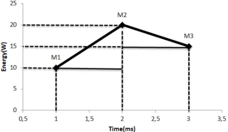
Measuring consumption with instant consumption readings
The information about the consumption of the Intel Xeon Phi and the NVIDIAGPUs is ob-tained in Watts instead of Joules, i.e. instead of receiving the accumulated energy like in the Intel processors the value received is the current power. To calculate the energy consump-tion of these coprocessors, a minimum of two different power readings have to be collected. A simple example can be viewed in Figure 3 where 3 measurements are taken within 2
milliseconds. To calculate the total energy consumption of the device the consumption be-tween every reading is computed. In the example of Figure 3 the consumption between
measurements M1 and M2 and M2 and M3 correspond to the total energy consumption. Each of these consumptions can be easily calculated as the sum of the area of a right trian-gle with the area of a rectantrian-gle, which is used as an approximation to the integral of the energy consumption. Equation3describes how the total energy consumption between two
measurements is calculated.
ConsumptionMiMj =min(Miconsum, Mjconsum) ∗ (Mjtime−Mitime)
+ ((max(Miconsum, Mjconsum)
−min(Miconsum, Mjconsum))
∗ (Mjtime−Mitime)/2)
(3)
The total consumption between the first measurement and measurement N is calculated as shown in Equation4. totalConsumptioM1Mn = n−1
∑
i=1 ConsumptionMiMi+1 (4)3.1. The scheduler model 21
For this example the total energy consumption between M1 and M2 would be:
consumptionM1M2 =min(10, 20) ∗ (2−1) + ((max(10, 20) −min(10, 20)) ∗ (2−1)/2)
=10∗1+ ((20−10) ∗1/2)
=10+5
=15mJ
Similarly, between M2 and M3 the consumption would be:
consumptionM2M3 =min(20, 15) ∗ (3−2) + ((max(20, 15) −min(20, 15)) ∗ (3−2)/2)
=15∗1+ ((20−15) ∗1/2)
=15+5
=20mJ
So the total consumption in this example would be 35 mJ (15 + 20).
Figure 3.: Consumption calculation with instant consumption readings
3.1.1 Scheduling decisions
Since the scheduler can not apply any scheduling technique directed at an individual task, it can only choose which task type is better for each worker, accordingly to the scheduling decision selected by the user. To choose the best task type for each worker, a sort is made to each of the lines in the relations table (that corresponds to each worker) where the compare function is chosen by the user. Currently there are 6 different compare function available:
• Energy consumption per FLOP - focuses on reducing the energy consumption per
3.1. The scheduler model 22
• Energy consumption per byte - focuses on reducing the energy consumption per byte handled
• Energy consumption - focuses on reducing the energy consumption of the tasks over-all
• Performance perFLOP- focuses on maximising the throughput perFLOPoperation
• Performance per byte - focuses on maximising the throughput per byte of memory handled
• Performance - focuses on maximising the throughput per task
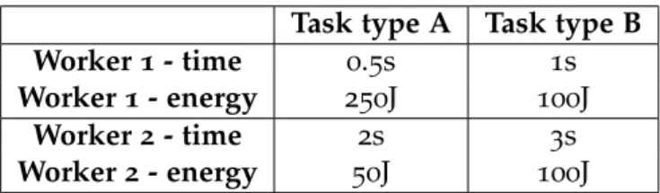
Task type A Task type B
Worker 1 - time 0.5s 1s
Worker 1 - energy 250J 100J
Worker 2 - time 2s 3s
Worker 2 - energy 50J 100J
Table 1.: Relation table values for the scheduling decision combination example
There was an attempt to combine two or more different scheduling decisions by calculat-ing the fitness percentage of each task type for each worker on both schedulcalculat-ing decisions and then combining the percentages accordingly to weights defined by the user. The fitness for each scheduling decision is calculated by the value in the relations table divided by the sum of all the values on the same line of the relations table (corresponding to all the values of the same type (energy, time, energy/FLOP, ...) for a given worker). For example, with two task types A and B and two workers 1 and 2, and with the values of the relations table presented in table 1the computations of the task type’s fitness on worker 1 would be
calculated the following way:
• Case 1 - the scheduling decisions selected were energy consumption and performance and the weight of both is 50%:
FitnessPer f ormanceTypeA=0.5/1.5
=33.33% FitnessConsumptionTypeA=250/350
3.1. The scheduler model 23
FitnessPer f ormanceTypeB=1/1.5
=66.67% FitnessConsumptionTypeB=100/350
=28.57%
Since both time per task and consumption need to be minimised, the task type with the smaller percentage value will be selected:
OverallFitnessTypeA= (33.33∗0.5+71.43∗0.5) =52.38%
OverallFitnessTypeB= (66.67∗0.5+28.57∗0.5) =47.62%
In this case the scheduler would assign tasks of type B to worker 1 on the current iteration.
• Case 2 - the scheduling decisions selected this time were still energy consumption and performance by this time the weight is of 70% to performance and 30% to energy consumption. The fitness of the task types for a single scheduling decision are the same as the example above, with only the combination between them changing. The task type selected will still be the one with the smallest percentage:
OverallFitnessTypeA= (33.33∗0.7+71.43∗0.3) =44.76%
OverallFitnessTypeB= (66.67∗0.7+28.57∗0.3) =55.24%
This time the worker 1 will be assigned tasks of type A, since it has the smallest percentage.
3.2. Scheduling tuning 24
Unfortunately there was no time to properly test the combination between different scheduling so it is not presented on section 4.2. The proper testing of this algorithm is
suggested as future work.
3.2 s c h e d u l i n g t u n i n g
When the scheduler starts, it collects information about the workers present in the sys-tem. The information about theCPUis collected by accessing the /proc/cpuinfo file on Linux which can tell the number of sockets and the number of cores per socket. The GCC compiler command ”gcc -march=native -Q –help=target—grep march” is also used to obtain information about the family of theCPU. For information about the Xeon Phi devices, the micinfo com-mand is used. Finally for detecting graphic cards the nvmlUnitGetCount function, which is part of theNVMLlibrary, is called.
Since there is no more information in the beginning and the relations table is empty. A tuning stage is used to populate the information of the relations table and in some entries of the history list. Three different ways of tuning the scheduler were created. All tuners have the same behaviour where a block of tasks of the same type is analysed in each worker on each tuning iteration.
The tuning technique currently available are the following:
• By block - in this tuning technique the user defines how many tasks (in constant number) are used by each worker in each iteration
• By percentage - in this tuning technique the user defines a percentage of tasks that are assigned in each training iteration. The difference between this training and the training by block is that task types with different number of tasks will have different block sizes
• By time - in this tuning technique the user defines a time (in seconds) in which each worker tests as much tasks as it can of the same type. The scheduler assigns tasks to the workers and wait for the workers to finish to assign them more tasks. If the time defined by the user has already passed, the scheduler stops assigning tasks.
3.3 t h e s u p p o r t f r a m e w o r k
Since the simulator presented in Section2.2.1is not able to accurately simulate the energy
consumption of heterogeneous tasks and workers, a framework was created to test the be-haviour of the scheduler when altering the scheduling parameters and to test the potential
3.3. The support framework 25
of using time and power consumption measurements to schedule the following iterations. This framework was created to be able to fully monitor the time and the consumption of the tasks on each device while having least impact possible on the overall computational time.
Since the framework was created with the goal of testing different tuners and scheduling techniques each of the tuners and scheduling decisions can be easily replaced. Even the scheduling algorithm itself can be easily changed if needed.
The algorithm used for assigning tasks, starting the workers and doing all the measure-ments is presented in Algorithm1. The algorithm in the case of the tuners is very similar to
Algorithm1 but there is no need to choose the best task type since all the task types have
to be sampled and there is also no need to choose the workload for each worker because it is chosen by the user, unless the user chooses the timed trainer. When the scheduler needs to calculate the base workload for a history combination that was not used before, the algo-rithm2is used. Algorithm 2does not provide any guarantees about the load balancing, it
only calculates the total base workload (the workload for all the workers combined) based on the number of tasks in the queue. As can be seen in Algorithm 1, the only difference
in the behaviour of the different scheduling decisions currently available is the ordering of the best task types for each worker at the end of each iteration.
Data: workers; queue of tasks; relations; history; scheduling decision
Result: all the tasks for the iteration are assigned and run and the measurements about time and energy consumption are made
while there are still tasks in the queue do
compute the best task type for each worker based on the relations; compute the best workload for the workers based on the history; assign tasks to the workers;
start the iteration timer; forall workers with work do
start a thread running each worker’s work function; end
wait for all the workers to finish; stop the iteration timer;
forall workers do
store the information about the last iteration in the relations and history structures;
end
sort each relation table line accordingly to the scheduling decision selected; end
3.3. The support framework 26
Data: the total number of tasks on a single task type queue
Result: the base workload for that task type based on the size of the queue initiate the variables (i and n, both int);
for n = 0; i≤queueSize; ++n do i = 10n;
end
return queueSize / 2n;
Algorithm 2:Calculation of the base workload for a single task type queue
The function that handles the work of each worker is presented in Algorithm3. It simply
starts the power reader associated with the device and a time counter before the worker starts working. The power reader and time counter are stopped after all the work assigned to the worker this iteration is complete. Similarly when measuring the number of FLOP
inside the tasks, aFLOPcounter usingProcess API (PAPI)is started and stopped only when all the work is complete.
Data: worker
Result: the worker finishes it’s work and stores information about the iteration so it can be handled by the scheduler
start a thread with the power sampler of the worker; start a timer;
while there is still work in the worker’s queue do do the task’s work;
end
stop the power sampler’s thread and the timer;
store the information about time, power consumption and work done; Algorithm 3:Work function of the worker
Since there are three different tuning techniques, six different scheduling decisions and other variables an additional structure was created to serve as a control structure for the framework, decreasing the amount of work the user needs to do before being able to run the code on the framework. This control structure detects the devices available in the system (number of CPUs, GPUs and coprocessors, the number of cores available on each device and also the family of the processor used in the system, which is needed for the power reader (the default value for the processor family is Sandy Bridge)) and receives and han-dles the choices of the user relative to the tuner and scheduling decision selected.
To use this framework, the user must create a new project and link the scheduling or the power sampler libraries. Each of the task types created must be extensions of the task base class available on the scheduler libraries in order to use the scheduler. Since there is no memory control, the user has to define how the data is transferred to the devices. Each task
3.3. The support framework 27
returns the number of bytes handled to and from the devices which is used to simulate part of a memory control and allows the scheduler to make decisions based on the number of bytes handled. The value of number of bytes handled is provided by the user as the return of the task (this was only done to be able to test the scheduling decisions that need the number of bytes handled as an argument).
4
T E S T A N D E VA L U AT I O NThe key motivation to develop a new framework was the lack of a real-time tools that can take in-time scheduling decisions considering not only the measured devices performance but their energy consumption as well. To evaluate the quality of the framework outcomes several tests were devised and applied, and their results are here presented and discussed.
All tests used two different task types: squared matrix multiplication and theSingle Preci-sion A.X Plus Y (SAXPY)algorithm. These tasks are both regular, where the amount of data transfers and computations can be found by knowing the size of the matrices and vectors. With regular tasks the workload balancing between devices should be very effective. Both tasks are implemented using MKL for both multicore and many-core Xeon devices and using cuBLAS for the implementation on the NVidia GPUs.
The first set of tests aimed to find out the performance and energy consumption of each device (and all the combinations between them) when running SAXPY tasks. To test the behaviour of the devices when handling SAXPY tasks 5 different array sizes were tested (16k, 32k, 64k, 128k and 256k). For each of the tests, 1000 SAXPY tasks were ran. Two different comparisons were made with the results: in the first one different device combi-nations (CPU only, CPU and GPU, all workers, ...) were tested for arrays with the same size; in the second the different task sizes were compared for the same worker combination.
The second set of tests, similar to the first, was done to test the behaviour of each device when running matrix multiplication tasks. Once again 5 different sizes were tested with the number of elements varying between 64k, 256k, 1M, 4M and 16M. Since the matrix mul-tiplication tasks have much more operations than the SAXPY tasks, the number of tasks on each test was set to 200. With a small number of tasks, the scheduler does not have many iterations to find the best tasks for each worker and the balance between them so the scheduler needs to be able to quickly find a good balance.
4.1. Testbed 29
The third set of tests combined the previous two and was done to evaluate the behaviour of the scheduler when having two different task types to choose from when assigning work to each of the devices.
For these tests the scheduling decision used was the power consumption, the tuner se-lected was the tuner by block with a block of 10 tasks. The update rate chosen was 80 per cent. The rate of readings for each power sampler is 1 millisecond, the lowest possible for all of the device power samplers.
4.1 t e s t b e d
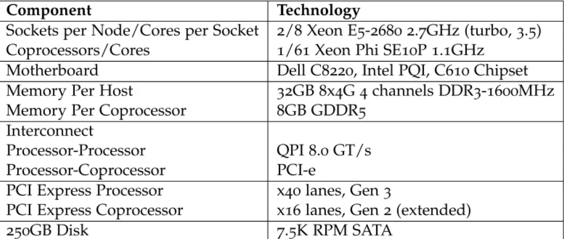
The testbed where the framework will be tested is one of the nodes available on the Stam-pede supercomputer which is one of the supercomputers available at Texas Advanced Com-puting Center (TACC). The Stampede supercomputer is comprised of 6404 nodes of which 4 are login nodes and the other 6400 are computation nodes. Table 2 shows the
config-uration of each of he 6400 nodes and Table 3 shows the overall system configuration and
performance (these tables were obtained from the Stampede User Guide, available inTACC
(2017)). As can be seen in Table2each compute node has two Intel Xeon E5-2680 on a single
board, as aSymmetric multiprocessing (SMP)unit with a performance of 346 GFLOPS/node. Additionally each node has a special production Intel Xeon Phi SE10P with a peak perfor-mance of 1.0 DP TFLOPS/Phi. Each node contains 32GB of memory, with 4 channels from each processor’s memory controller to 4 DDR3 ECC DIMMS, obtaining 51.2GB/s for all four channels in a socket. The memory for each coprocessor is 8GB GDDR5 with 8 dual-channel controllers and a peak performance of 320GB/s.
Component Technology
Sockets per Node/Cores per Socket 2/8 Xeon E5-2680 2.7GHz (turbo, 3.5) Coprocessors/Cores 1/61 Xeon Phi SE10P 1.1GHz
Motherboard Dell C8220, Intel PQI, C610 Chipset Memory Per Host 32GB 8x4G 4 channels DDR3-1600MHz Memory Per Coprocessor 8GB GDDR5
Interconnect
Processor-Processor QPI 8.0 GT/s Processor-Coprocessor PCI-e
PCI Express Processor x40 lanes, Gen 3
PCI Express Coprocessor x16 lanes, Gen 2 (extended)
250GB Disk 7.5K RPM SATA