Uso de redes neurais artificiais para predição da evapotranspiração no cultivo protegido de pimentão

Revista Brasileira de

Engenharia Agrícola e Ambiental

Campina Grande, PB, UAEA/UFCG – http://www.agriambi.com.br

v.20, n.6, p.507-512, 2016

Artificial neural networks employment in the prediction

of evapotranspiration of greenhouse-grown sweet pepper

Héliton Pandorfi

_{, Alan C. Bezerra}

_{, Roberto T. Atarassi}

_,

Frederico M. C. Vieira

_{, José A. D. Barbosa Filho}

_{& Cristiane Guiselini}

A B S T R A C T

This study aimed to investigate the applicability of artificial neural networks (ANNs) in the prediction of evapotranspiration of sweet pepper cultivated in a greenhouse. The used data encompass the second crop cycle, from September 2013 to February 2014, constituting 135 days of daily meteorological data, referring to the following variables: temperature and relative air humidity, wind speed and solar radiation (input variables), as well as evapotranspiration (output variable), determined using data obtained by load-cell weighing lysimeter. The recorded data were divided into three sets for training, testing and validation. The ANN learning model recognized the evapotranspiration patterns with acceptable accuracy, with mean square error of 0.005, in comparison to the data recorded in the lysimeter, with coefficient of determination of 0.87, demonstrating the best approximation for the 4-21-1 network architecture, with multilayers, error back-propagation learning algorithm and learning rate of 0.01.

Uso de redes neurais artificiais para predição

da evapotranspiração no cultivo protegido de pimentão

R E S U M O

Este trabalho foi conduzido com o objetivo de investigar a aplicabilidade das redes neurais artificiais (RNAs) para estimar a evapotranspiração do cultivo protegido de pimentão. Os dados utilizados compreenderam o segundo ciclo da cultura, cultivado de setembro de 2013 a fevereiro de 2014, constituindo 135 dias de dados meteorológicos diários: temperatura e umidade relativa do ar, velocidade do vento e radiação solar global, utilizadas como variáveis preditoras e evapotranspiração, determinada a partir de dados obtidos por lisímetro de pesagem, usada como variável resposta. Os dados registrados no período foram divididos em três conjuntos para treinamento, teste e validação. O processo de aprendizado da RNA foi estabelecido com precisão aceitável, com erro médio quadrático de 0,005, em que os padrões de evapotranspiração no ambiente protegido estimado pela rede, em comparação àqueles gerados a partir dos dados de lisimetria, apontaram coeficiente de determinação da ordem de 0,87 para uma arquitetura de rede 4-21-1, de múltiplas camadas, algoritmo de aprendizagem de retropropagação do erro e taxa de aprendizagem de 0,1.

Key words:

microclimate sweet pepper expert system computational vision

Palavras-chave:

microclima pimentão

sistema especialista visão computacional

1 _{Universidade Federal Rural de Pernambuco/Departamento de Engenharia Agrícola. Recife, PE. E-mail: heliton.pandorfi@ufrpe.br; cguiseli@hotmail.com}

(Corresponding author)

2 _{Universidade Federal Rural de Pernambuco/Unidade Acadêmica de Serra Talhada. Serra Talhada, PE. E-mail: cezaralan.a@gmail.com} 3 _{Universidade Federal de Uberlândia/Instituto de Ciências Agrárias. Uberlândia, MG. E-mail: robertota@ufu.br}

4 _{Universidade Tecnológica Federal do Paraná/Coordenação do Curso de Agronomia. Dois Vizinhos, PR. E-mail: fredericovieira@utfpr.edu.br} 5 _{Universidade Federal do Ceará/Centro de Ciências Agrárias/Departamento de Engenharia Agrícola. Fortaleza, CE. E-mail: zkdelfino@gmail.com}

Introduction

In the last years, the rational use of water has increasingly received attention due to the water scarcity problems faced by many regions of the country. Freshwater is a renewable natural resource and has regional and seasonal variations (Augusto et al., 2012). Besides this variation, it is known that a considerable part of the water extracted from the sources does not reach its destination due to infrastructure problems, which worsens the problem with water.

In addition, it should be pointed out that agriculture is one of the sectors that most demand water for their activities. Thus, with the gradual increase in cultivated areas and the scarcity of water resources, it is necessary to use techniques and technologies for the rationalization of water consumption (Silva et al., 2014). Therefore, the adoption of a management that meets crop water requirements and the use of technologies that reduce the consumption, such as protected environments, stand out.

For the protected environment to promote the benefit of water economy, it is essential the knowledge on evapotranspiration and crop water requirement for its correct replenishment (Kumar et al., 2011). Since the protected environment modifies the micrometeorological characteristics of the internal environment, some commonly used methods of evapotranspiration estimation are not adequate, such as the Bowen ratio and the aerodynamic method (Hanan, 1998). Therefore, studies have determined water consumption through lysimetric (weighing and drainage lysimetry) and gravimetric methods, relating them to variables from the internal environment and the crop (Oliveira et al., 2014).

Other methodologies have been developed for the application of modeling and the use of computational tools, for micrometeorological management in protected environments. One of the first reports in the literature was the research of Businger (1963), which originated methods aimed at the optimization of mass and energy flows and estimation of temperature, air humidity and evapotranspiration (Kimball, 1973; Avissar & Mahrer, 1982).

The simplification of methods has been achieved through computational vision with the use of artificial neural networks (ANNs), because it is a flexible mathematical structure that allows identifying the non-linear relationships between input and output data (Shirigure, 2013). A few studies have proposed neural networks to determine reference evapotranspiration for various localities.

In order to estimate reference evapotranspiration in the state of Rio de Janeiro, Zanetti et al. (2008) used a neural network considering geographic coordinates and air temperature. Rahimikhoob (2010) proposed a neural network for the determination of reference evapotranspiration (ET0) under humid subtropical conditions in North Iran, using maximum and minimum air temperatures, as well as global solar radiation. Alves Sobrinho et al. (2011) developed an ANN capable of estimating ET0 through data of daily air temperature for the region of Mato Grosso do Sul and, in one of the mentioned studies, the authors observed excellent results for the estimation of ET₀.

In the development of their research, Abedi-Koupai et al. (2009) aimed to evaluate reference evapotranspiration in a protected environment, comparing the results of a ANN with other conventional methods using as a reference the evapotranspiration obtained with drainage lysimeter. The results showed that the neural network obtained the best adjustment, compared with the conventional methods.

The need for such bidirectional information flow, data collection and decision making requires the use of information technology at different scales and strategies of integration of systems based on open patterns, with emphasis on irrigation management automation. Thus, this study aimed to investigate the applicability of ANNs in the prediction of evapotranspiration of sweet pepper grown in a protected environment.

Material and Methods

The study was carried out at the Department of Biosystems Engineering of the “Luiz de Queiroz” College of Agriculture (ESALQ) of the University of São Paulo, in the city of Piracicaba, SP, Brazil (22° 42' 00'' S; 47° 38' 00'' W; 520 m).

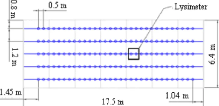
The database used in the study was obtained in a protected environment, a simple arched-roof East-West oriented structure, with length of 17.5 m, width of 6.4 m, ceiling height of 3.0 m and arch height of 1.2 m, covered with 0.15-mm-thick low-density polyethylene (LDPE) film. The sides consisted of shade screens (60%) and curtains, with the same plastic film of the cover and mechanism of opening and closure.

The soil in the area was classified as Nitosol (EMBRAPA, 2006). The sweet pepper variety “Matador” was used in the data recording stage of the experiment. The crop was planted in single rows, at the spacing of 0.5 m between plants and 1.2 m between rows (Figure 1), in a total of 155 plants.

The experiment used an ‘inverted-V’ staking system, with four stakes per plant, supported by fence posts at the ends of the rows and rafters screwed at 1.9 m from the soil, where a set of steel wires was tensioned. Bamboo sticks were fixed at a spacing of 2.5 m between stakes along the planting row.

The soil was prepared with a basal fertilization, according to soil analysis and the recommendation of the Bulletins 100 and 200 of the Agronomic Institute of Campinas (IAC), by applying 2 kg m-2 _{of aged cattle manure and 0.015 kg of P}

2O5 m-2 _{in the form of magnesium thermophosphate and the} recommended amounts of micronutrients. After application, the material was incorporated using a micro-tractor with

rotary hoe and the beds were constructed. Then, the irrigation system was installed with pressure-compensating drip lines, with emitters spaced by 30 cm, flow rate of 1.6 L h-1 _{per emitter} and one drip line per crop row. A separate line with a valve was connected to the lysimeter tank, which allowed independent management. The system was activated by a 0.5-hp motor pump set connected to three water tanks, one of 1000 L and two of 500 L.

The beds were covered with double-faced, silver-colored plastic mulch, composed of 1.5-m-wide polyethylene film, with the black side facing the soil and the silver side facing the environment. The mulch was used to reduce soil evaporation, conserving moisture and inhibiting the occurrence of weeds.

After planting, the crop was subjected to fertigation with a solution of 0.2 g L-1 _{of potassium nitrate (13% of N and 42%} of K₂O) and 0.2 g L-1 _{of calcium nitrate (15.5% of N and 26.5%} of Ca). Fertigation management was based on the variation of mass of the load-cell lysimeter.

A data-acquisition system was installed and programmed for readings every 4 s and means recorded every 30 min, except the load cells of the weighing lysimeter, which recorded the mean of the last 10 min, representing the point mass every 30 min. Crop transpiration was recorded using a lysimeter with three load cells, with nominal capacity of 500 kg, sensitivity of 2 mV V-1 _{(±0.1%) and combined error lower than 0.03% of} the nominal capacity.

Global solar radiation was recorded by a pyranometer installed at 1.9 m from the soil, with measurement range from 0.3 to 3 µm. Wind speed (m s-1_{) close to the crop canopy was} determined using an ultrasonic anemometer. Psychrometric variables, such as temperature, actual vapor pressure, relative air humidity and vapor pressure deficit, were measured with aspirated thermocouple psychrometers, installed every 0.30 m along the canopy height, from 0.15 m of the soil level.

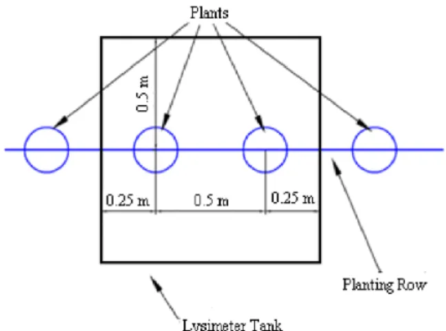
The weighing lysimeter consisted of a metallic container, 1.0 x 1.0 x 0.45 m (L x W x H), installed in one of the planting rows in the center of the protected environment, in order to minimize the oasis effect. The tank of soil was placed directly on the three load cells, which were fixed on a base made of steel profiles. The lysimeter was installed with two sweet pepper plants, as shown in Figure 2.

Field calibration was performed using weights with known masses and subsequent adjustment through multiple linear

regression. The surface of the soil tank was covered with a polyethylene film to eliminate evaporation, which could cause errors in the calibration. Readings were performed during both addition and removal of the weights, obtaining the following calibration equation, Eq. 1:

Figure 2. Scheme of sweet pepper planting in the lysimeter tank

( )

3

Mass kg 270.763Cell 242.996Cell 253.319Cell 851.564

= + +

+ −

where:

Cell1, Cell2, Cell3 - signals of the load cells, mV V -1_.

The regression showed a coefficient of determination of 0.99 and standard deviation of the estimate of 0.01 kg, which indicated optimal adjustment.

Crop evapotranspiration, ETc (mm h 1_{), was calculated} using lysimeter mass data, through Eq. 2:

ML ETc

t AL

∆ =

∆ ⋅

where:

ΔML - variation of lysimeter mass in the time interval, kg; Δt - time interval between readings, h; and,

AL - sampling area of the lysimeter, m2_.

The data recorded along the cultivation of sweet pepper in a protected environment, used in the prediction of evapotranspiration through neural networks, encompass the second crop cycle, from September 22, 2013 to February 4, 2014, constituting 135 days of daily meteorological data, referring to the variables temperature, relative air humidity, wind speed, solar radiation (input variables) and evapotranspiration (output variable), determined by the weighing lysimeter with load cells.

The neural networks were controlled using a dedicated computer program and the data recorded in the period were divided into three sets, 40% for training, 20% for test and 40% for validation. All the data were normalized [0,1] to facilitate the convergence during the ANN training process, Eq. 3. The model used in the present study for the development of the neural network was the error back-propagation algorithm (Haykin, 2001).

(

)

(

)

y y y

y y

− =

−

where:

y - normalized value of each variable; y₀ - actual value of each variable; and,

ymax and ymin - maximum and minimum values among the actual values of the variables.

The learning process was divided into three steps for which a distinct part of the input data was reserved: i) training - the synaptic weights were modified and the ANN model acquired the new knowledge; ii) test - the recently modified model was (1)

(2)

tested for its performance; and iii) validation - the model was tested, generating results for the new inputs. In order to obtain good adjustments, it was necessary to repeat the steps of training and test iteratively.

The synaptic weights were randomly initiated while the activation of the neurons followed the tangent-sigmoid function. The results were analyzed using, simultaneously, the mean square error (MSE) and the mean relative error (MRE), exclusively calculated for the validation set, i.e., for the set of data that were still new for the network.

The learning rule consisted in the minimization of MSE, which adjusts the weights of the connections between the neurons of the network according to the error. This rule aims to find a set of weights and polarizations that minimize the error function, Eq. 4.

relative air humidity, global solar radiation, wind speed and evapotranspiration, whose input matrix was 135 x 4 (135 observations with 4 variables) and output matrix was 135 x 1. After training many network configurations, the following topology was selected: 4 input variables (air temperature, relative air humidity, global solar radiation and wind speed), 21 neurons for each hidden layer and 1 for the output (evapotranspiration).

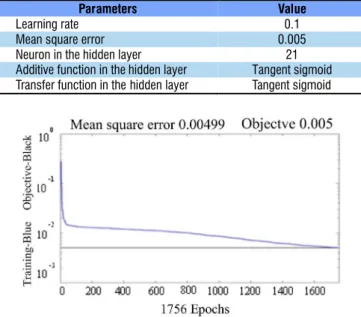
One of the problems in the training of multilayer neural networks with error back-propagation training algorithm was the definition of the parameters. Selecting the training parameters of the algorithm was a process that demanded great effort, since small alterations in these parameters led to large differences in both training time and the obtained generalization (Table 1).

The parameter learning rate showed great influence during the process of neural network training. A very low learning rate made the process very slow, while a very high learning rate caused oscillations in the training, which prevented the convergence of the learning process. In general, its value varies from 0.1 to 1.0; however, for the training of this neural network, a pre-fixed value of 0.1 was adopted, since higher values did not allow the convergence of the process on the MSE surface.

As to the number of neurons in the hidden layer, they were defined empirically; after various attempts, the value of 21 neurons was found, allowing the extraction of the general characteristics of the data set for good generalization, which showed optimal output, after its training.

The training was ended when there was convergence on the MSE surface, in which the value of 0.005 was adopted; after various adjustments as a function of the result, good generalization was achieved at 1756 cycles, i.e., the number of times that the training set was presented to the network (Figure 3).

The predictions in the training step showed mean value capable of simulating the peaks of the events; the prediction

(

)

R S ₂

' p,i p,i p 1 i 1

1

E y y

2 = =

=

∑∑

where:

R - number of input patterns or vectors;

S - number of output neurons - dimension of the output vector;

yp,i - desired output in the i-th neuron, when the p-th pattern is presented; and,

y’p,i - output obtained by the network in the i-th neuron, when the p-th pattern is presented.

The criterion adopted for the completion of the training was defined by a combination of methods, through the MSE of the estimate and the number of cycles, ending the training when one of the criteria was met. The training set was presented to the neural network for the error back-propagation algorithm to act, i.e., the algorithm performed many iterations of update of the weights until reaching the value of MSE of the estimate (0.005).

The main restriction in error minimization in the descen-ding gradient direction was that the neuron transfer function should be monotonic and differentiable at any point.

The error back-propagation algorithm showed learning rule that consisted in the adjustment of the network weights and polarizations, based on the error back-propagation found in the output. Minimization was achieved through the continuous update of the weights and polarizations in each interaction in the opposite direction of the function gradient at the current point, i.e., proportionally to the negative of the derivative of the square error in relation to the current weights. Therefore, it is a deterministic supervised training algorithm, which implemented the method of the descending gradient in the sum of the square errors.

The network architecture topology used was formed by an input layer, a hidden layer (intermediate) of non-linear neurons and one output layer of neurons with parameterized logistic-sigmoid-tangent activation function.

Results and Discussion

The formation layers of the network architecture were used in the approximation of the variables air temperature,

Figure 3. Data re-presentation cycles in the neural network training step

Parameters Value

Learning rate 0.1

Mean square error 0.005

Neuron in the hidden layer 21

Additive function in the hidden layer Tangent sigmoid Transfer function in the hidden layer Tangent sigmoid Table 1. Training parameters used for the error back-propagation algorithm

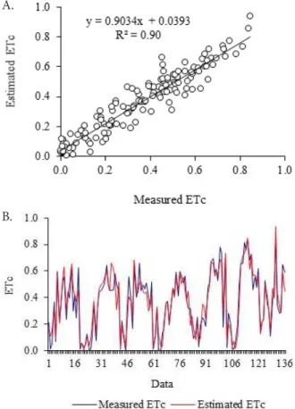
through the neural network allowed characterizing the variation of crop evapotranspiration, with coefficient of determination of approximately 0.90 (Figure 4A)

As general consideration of the training results, the approximations of the values estimated by the neural network showed optimal characterization of the actual data recorded along the experimental period, with only a few points at which there was a tendency to overestimate high values (Figure 4B).

Input and output pairs allowed observing the evolution of the learning through the comparison between the desired output and the actual value in the network test step. The patterns adopted for the generation of the model were able to simulate crop evapotranspiration, with coefficient of determination of 0.91 (Figure 5A).

Similar results were reported by Kumar et al. (2008) in the comparison between the ANN model and the methods of Hargreaves and Penman-Monteith (PM-56) for the estimation of reference evapotranspiration, with coefficient of determination of 0.90. The variation of measured and estimated crop evapotranspiration showed similar values and optimal generalization of the ANN-estimated data; at a few isolated points, the same variation profile was observed, which indicates small tendency to underestimate low values (Figure 5B).

Rahimihoob (2010) considered as acceptable values of over- and underestimation from 7 to 8%, with a 3-6-1 network architecture, for reference evapotranspiration data measured using the PM-56 equation and those estimated by the neural network in four localities of North Iran, with coefficients of determination ranging from 0.93 to 0.96. Considering underestimated values of sweet pepper evapotranspiration of

Figure 4. Functional relationship between the normalized data of ETc measured in the lysimeter and ETc estimated

by the artificial neural network (A) in the training step (B)

B. A.

Figure 5. Functional relationship of the normalized data of ETc measured in the lysimeter and ETc estimated by the

artificial neural network (A) in the test step (B)

B. A.

about 9%, such effect can be overcome by the increase in the number of daily observations, allowing greater reliability on the predicted results (Zanetti et al., 2007).

The predicted and measured values in the network validation step (Figures 6A and 6B) showed a data variation profile in which the noises were found within an acceptable range, evidenced by the coefficient of determination of approximately 0.87. Similar result was reported by Kumar et al. (2002) for the prediction of reference evapotranspiration at the field using a 6-7-1 network architecture and error back-propagation learning algorithm, obtaining coefficient of determination of 0.83 for the relationship between the data measured in the lysimeter and those predicted by the network. Abedi-Koupai et al. (2009) used two hidden layers with five neurons, each one with four input values, one output layer and log-sigmoid function, and obtained coefficient of determination of 0.95 for reference evapotranspiration in protected environment.

These results confirm that the application of ANNs allows the establishment of evapotranspiration patterns in protected environments; however, this specialist system must be periodically monitored regarding its performance, to maintain the network, or indicate to the user the need for a new training, according to the studies of Zanetti et al. (2007).

Figure 6. Functional relationship between the normalized data of ETc measured in the lysimeter and ETc estimated

by the artificial neural network (A) in the validation step (B)

B. A.

It is important to point out that other network architectures or other parameters can also be applied for similar situations and that the proposed solution was selected to present the potential of application of the tool and its good performance, with potential to integrate automated control systems in irrigation management for the cultivation of sweet pepper in protected environment.

Conclusions

1. The approximation problem served to demonstrate the viability of utilization of artificial neural networks for the prediction of sweet pepper evapotranspiration in protected environment, compared with that measured by the weighing lysimeter.

2. The 4-21-1 network architecture, with multilayers, error back-propagation learning algorithm and learning rate of 0.1, showed the best approximations for the estimation of evapotranspiration.

Literature Cited

Abedi-Koupai, J.; Amiri M. J.; Eslamian, S. S. Comparison of artificial neural network and physically based models for estimating of reference evapotranspiration in greenhouse. Australian Journal of Basic and Applied Sciences, v.3, p.2528-2535, 2009.

Alves Sobrinho, T.; Rodrigues, D. B. B.; Oliveira, P. T. S. de; Rebucci, L. C. S.; Pertussatti, C. A. Estimativa da evapotranspiração de referência através de redes neurais artificiais. Revista Brasileira de Meteorologia, v.26, p.197-203, 2011. http://dx.doi.org/10.1590/ S0102-77862011000200004

Augusto, L. G. D. S.; Gurgel, I. G. D.; Câmara Neto, H. F.; Melo, C. H. D.; Costa, A. M. O contexto global e nacional frente aos desafios do acesso adequado à água para consumo humano. Ciência & Saúde Coletiva, v.17, p.1511-1522, 2012. http://dx.doi.org/10.1590/ S1413-81232012000600015

Avissar, R.; Mahrer, Y. Verification study of a numerical greenhouse microclimate model. Transactions of the ASAE, v.25, p.1711- 1720, 1982. http://dx.doi.org/10.13031/2013.33794

Businger, J. A. The glasshouse (greenhouse) climate. In: Wijk, W. R. Physics of plant environment. Amsterdam: North Holland, 1963. p.277 -318.

EMBRAPA - Empresa Brasileira de Pesquisa Agropecuária. Centro Nacional de Pesquisa de Solos. Sistema brasileiro de classificação dos solos. 2.ed. Rio de Janeiro: Embrapa Solos, 2006. 306p. Hanan, J. J. Greenhouses: Advanced technology for protected

horticulture. Boca Raton: CRC Press, 1998. 684p.

Haykin, S. Redes neurais: princípios e práticas. 2.ed. Porto Alegre: Bookman, 2001. 900p.

Kimball, B. A. Simulation of the energy balance of a greenhouse. Agricultural Meteorology, v.11, p.243 -260, 1973. http://dx.doi. org/10.1016/0002-1571(73)90067-8

Kumar, M.; Bandyopadhyay, A.; Raghuwanshi, N.S.; Singh, R. Comparative study of conventional and artificial neural network-based ETo estimation models. Irrigation Science, v.26, p.531-545, 2008. http://dx.doi.org/10.1007/s00271-008-0114-3

Kumar, M.; Raghuwanshi, N. S.; Singh, R. Artificial neural networks approach in evapotranspiration modeling: A review. Irrigation Science, v.29, p.11-25, 2011. http://dx.doi.org/10.1007/s00271-010-0230-8

Kumar, M.; Raghuwanshi, N. S.; Singh, R.; Wallender, W. W.; Pruitt, W. O. Estimating Evapotranspiration using Artificial Neural Network. Journal of Irrigation and Drainage Engineering, v.128, p.224-233, 2002. http://dx.doi.org/10.1061/(ASCE)0733-9437(2002)128:4(224) Oliveira, E. C.; Carvalho, J. D. A.; Almeida, E. F.; Rezende, F. C.; Santos, B. G. dos; Mimura, S. N. Evapotranspiração da roseira cultivada em ambiente protegido. Revista Brasileira de Engenharia Agrícola e Ambiental, v.18, p.314-321, 2014. http://dx.doi.org/10.1590/ S1415-43662014000300011

Rahimikhoob, A. Estimation of evapotranspiration based on only air temperature data using artificial neural networks for a subtropical climate in Iran. Theoretical and Applied Climatology, v.101, p.83-90, 2010. http://dx.doi.org/10.1007/s00704-009-0204-z

Shirgure, P. S. Evaporation modeling with artificial neural network: A review. Scientific Journal of Review, v.2, p.73-84, 2013.

Silva, A. R. A.; Bezerra, F. M. L.; de Freitas, C. A. S.; Amorim, A. V.; de Carvalho, L. C. C.; Pereira Filho, J. V. Coeficientes de sensibilidade ao déficit hídrico para a cultura do girassol nas condições do semiárido cearense. Revista Brasileira de Agricultura Irrigada, v.8, p.38-51, 2014. http://dx.doi.org/10.7127/rbai.v8n100185 Zanetti, S. S; Sousa, E. F.; Carvalho, D. F.; Bernado, S. Estimação da

evapotranspiração de referência no Estado do Rio de Janeiro usando redes neurais artificiais. Revista Brasileira de Engenharia Agrícola e Ambiental, v.12, p.174-180, 2008. http://dx.doi. org/10.1590/S1415-43662008000200010