ABSTRACT: The application rate of plant-protection products is indicated as a concentration or amount of product per area. Greenhouse crops grow swiftly, and an application rate based on a fi xed amount of product per hectare can result either in large losses and overdoses when the plants are small or to be insuffi cient when the plants are fully developed. To solve these problems, the application rates of plant-protection products need to be adapted to the plant mass present in the greenhouse when the spray is applied. Two models were developed to estimate the leaf area based on easily measured geometric data of the vegetation in a greenhouse tomato crop. The model based on the PRV (Plant Row Volume) had that best results. The calculation of the vol-ume application rate from the PRV has resulted in a reduction of more than 30 % of the quantity of plant protection product sprayed, without decreasing yield. The PRV of a greenhouse tomato (Lycopersicon esculentum Mill.) is an easily measured parameter that enables the estimation of the leaf area index and the use of application strategies adapted to the changes in the plant canopy, saving major amounts of plant protection product used, compared to the conventional system.
Introduction
Quantifying vegetation and its subsequent relation to the spray-application rate are the basis for techniques of crop adapted spraying (CAS) used by researchers (Sut-ton and Unrath, 1988; Giles et al., 1989; Rüegg et al., 1999; Gil et al., 2007; Pergher and Petris, 2008) for ap-plying plant protection products in different crops. The goal is to achieve a more rational use of sprays according to the real needs of the crop while seeking to protect the environment and human health.
Different methods have been developed to solve the problems of adjusting the application rate to the level of crop development. One method is the “Tree-Row Vol-ume” (TRV) (Byers et al., 1971), whereby the applica-tion rate is determined by comparing the crop canopy volume per surface-area unit with the rate applied to a standard crop. This method specifi es the application rates in a more methodical way and has rendered good results in orchards (Sutton and Unrath, 1988; Rüegg et al., 1999; Gil et al., 2007; Siegfried et al., 2007). A sim-pler system was proposed by Furness et al. (1998), called “Unit Canopy Row” (UCR), in which the application rate was determined by each unit of 100 m3. Barani et al.
(2008)used the UCR in vineyards to determine the ap-plication rates and obtained good results.
To match application rates and spray volume, Weisser and Koch (2002) proposed the “treated area” concept, defi ned as the area that is sprayed and oriented between nozzles and targets. Therefore, for high crops the application rate is to be expressed in terms of the “leaf wall area” (LWA) (Koch, 2007).
Another way of establishing the application rate as a quantity of spray product per unit of leaf surface area is from the measurement of the LAI (Leaf Area Index). This parameter is used to determine the application rates (Dammer et al., 2008; Pergher and Petris, 2008; Gil and
Escolà, 2009). However, the use of the LAI to adjust the application rate is not very practical because its value is diffi cult to determine for the farmer under fi eld condi-tions.
This study describes a model to estimate the leaf area based on easily measured geometric data of the vegetation in a greenhouse tomato crop, such as the can-opy height or the Plant Row Volume (PRV), and its use to calculate the volume application rate of plant protection product from the average foliar deposit.
Materials and Methods
Measurement of geometric parameters of the canopy
This study was conducted with the geometric data from greenhouse tomato plants (Lycopersicon escu-lentum Mill.), measured at three locations from various commercial cultivars and in different types of green-houses, from 2007 to 2010. Table 1 lists the locations of the greenhouses, cultivars, and planting pattern of the crop. In all cases, the crop was planted in twin-rows (two plants per position) on a perlite substrate. In the greenhouses, the geometric parameters of height and width of the canopy as well as the foliar surface area were recorded using the methodology detailed below. These parameters were measured periodically (every 15-20 days) according to the crop cycle, development, and cultivation tasks.
Determination of the Plant Row Volume
The TRV is defi ned as the volume of vegetation per unit of surface area cultivated. In the present study, this is called Plant Row Volume (PRV), as this refers to annual plants and not to the trees, with the implications that this involves. The geometric variables needed to de-termine this index are height and width of the canopy, Received November 28, 2012
Accepted June 28, 2013
1University of Almería – Dept. of Agricultural Engineering,
Ctra. Sacramento s/n – 04120 – Almería – Spain.
2Andalusian Institute for Research and Training in Agriculture
(IFAPA-La Mojonera), Andalusian Government, Camino de San Nicolás, 1 – 04745 – La Mojonera, Almería – Spain. *Corresponding author <[email protected]> Edited by: Daniel Scherer de Moura
Volume application rate adapted to the canopy size in greenhouse tomato crops
and the distance separating the plant rows. Because the width of the canopy varies with plant height, PRV was calculated considering the volume of the vegetation cor-responding to each of the three heights defi ned to mea-sure the width (Figure 1). Thus, the PRV was calculated according to Eq. 1.
1 2 1 2 1 2
10000 H B B M M A A
PRV
3 D
(1)
where PRV is the Plant-Row Volume (in m3 ha–1), H is
the canopy height (in m), B1 and B2 are the width of the plants at 1/6 the height (in m), M1 and M2 width of the plants at 1/2 the height (in m), A1 and A2 width of the plants at 5/6 the height (in m) and D is the distance be-tween the rows (in m).
The height of the canopy was measured perpen-dicular to the soil. In the fi rst stages total height was considered. After the different clearing of leaves closest to the soil during the crop cycle, usual in cultiva-tion tasks, this measurement refers only to the zone with the foliar mass. The canopy height was measured in four randomly assigned pairs of plants representative of the rest of the greenhouse.
As the plants were paired, the width was the mean length parallel to the soil, from the lateral exte-rior of the right-hand plant to the lateral exteexte-rior of the left-hand plant, discounting the space between them, but without overestimating this geometric parameter (Figure 1).
Determination of the leaf area index
The surface area of the leafl ets comprising the leaves was measured, using a destructive method, which consisted of cutting off all the leaves of the individual, measuring their surface area with the use of a planimeter (WinDias, Delta-T Devices Ltd. Cambridge). Thus, this method involves the destruction of the studied sample. This parameter was measured on six plants assigned
at random from among the four pairs of plants used to measure the height and width. Because of the destruc-tion involved over the crop cycle, this parameter was not measured on all the plants.
Development of the model to estimate the LAI Models were developed to relate the canopy height, PRV, and LAI, with the aim of fi nding a correla-tion between them, and to be able to estimate LAI from the canopy height or from the PRV. For the development of these models, the mean values of H, PRV, and LAI were used for each greenhouse and day sampled, and were measured according to the methodology described above. Correlation and regression analyses were calcu-lated with the software SPSS v15.0 (SPSS Inc., an IBM Company, Chicago, IL, USA).
The accuracy of the developed models was deter-mined by measuring the height of the canopy and quan-tifying the LAI and PRV, according to the methodology
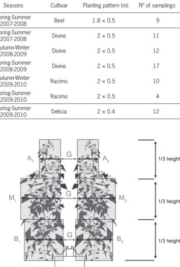
Table 1 – Geographical coordinates, season, and cultivar at the locations.
Locations Geographical coordi-nates WGS84 greenhousesNº of Area (m2) Seasons Cultivar Planting pattern (m) Nº of samplings
1 Lat. 36.84º
Long. -2.41º 1 8,000
Spring-Summer
2007-2008 Beel 1.8 × 0.5 9
2 Long -2.72ºLat. 36.79º 2 1,780
Spring-Summer
2007-2008 Divine 2 × 0.5 11
Autumn-Winter
2008-2009 Divine 2 × 0.5 12
Spring-Summer
2008-2009 Divine 2 × 0.5 17
Autumn-Winter
2009-2010 Racimo 2 × 0.5 10
Spring-Summer
2009-2010 Racimo 2 × 0.5 4
3 Long -2.71ºLat. 36.78º 2 1,920 Spring-Summer2009-2010 Delicia 2 × 0.4 12
Figure 1 – Measurement of width; B low width (B1+B2) (1/6 height),
M middle width (M1+M2) (1/2 height), and A high width (A1+A2) (5/6
of average foliar deposition in µL cm–2 leaf area (d v) the
volume application rate (V, in L ha–1) can be determined
by Eq. 5.
V = 2 . 10
2. d
V
. LAI/
ε
(5)The value of depends on sprayer type, crop struc-ture, and weather conditions. In several studies the values of dv and have been calculated in a greenhouse tomato crops (Cerruto et al., 2009a, b; Sánchez-Hermosilla et al., 2011, 2012), as indicated in Table 3. In consideration of these values, our proposal is to use a value of 1.5 µL cm–2
dv and, for the spray fraction deposited on the canopy () 0.50 for spray-gun applications or 0.75 for spray boom applications.
The value of LAI in Eq. 5 can be calculated with the model for estimating LAI as a function of geometric parameters of the crop, developed under the previous point.
Evaluation of the method to determine the volume application rate
To evaluate the method to determine the volume application rate, two greenhouses of 960 m2 (24 m × 40
m) were selected in La Mojonera, Almería, Spain, (36º48’ N, 2º41’ W and 142 m elevation) for a fi eld experiment during two seasons (spring-summer 2011 and autumn-winter 2011-2012). The crop used was tomato grown in perlite and planted in a twin-row system. Each twin-row was 2 m apart and had 50 pairs of plants spaced on 0.4 m (2.5 plants m–2).
Every greenhouse was divided into two blocks following a randomized block design with four blocks and two treatments (two application strategies). The treatments were the “conventional (CON)” and “esti-mated (EST)” application rate. The CON treatment in-volved spraying throughout the season according to the farmer’s criteria (application rate, pressure, travel speed, etc.). The EST treatment meant spraying according to the volume application rate calculated using the Eq. 5. During the application of the sprays, the concentration described above, in a tomato crop at 11 times over the
crop cycle (Table 2). The tomato cultivar was Divine, cul-tivated in a greenhouse in El Ejido, Almería, Spain (36º 48’ N, 2º 43’ W and 151 m elevation), during the au-tumn-winter season 2010-2011. For each of the develop-mental stages of the crop in which the data were taken, the LAI was estimated according to models established previously, and the prediction residual sum of squares (PRESS) was calculated using Eq. 2.
21
ˆ N
j j
j
PRESS LAI LAI
(2)where N is the total number of data (11); LAIj the known LAI for the j-th data and LÂIjthe estimated LAI of LAIj. The PRESS values provide a measure of how well the models predict the LAI. The prediction error of a LAI was calculated as the relative standard error (RSE) of the LAI prediction (Eq. 3).
2 121
2 1
ˆ
100
N
j j j
N j j
LAI LAI
RSE(%)
LAI
(3)Estimation of the volume application rate
Pergher and Petris (2008) proposed Eq. 4 to esti-mate the product application rate (Q, in g ha–1) based on
LAI, the average foliar deposit (d, in µg cm–2 leaf area)
and the spray fraction deposited on the canopy ().
Q = 2.102 . d . LAI/ (4)
The use of Eq. 4 to adjust the product application rate is not very practical because the values of LAI, d and are diffi cult to determine by the farmer under fi eld conditions. In the present study, the d value corresponds to the mean deposition achieved by farmers in their rou-tine practice, consisting of spray gun applications at high pressures and volumes. Taking into account the value
Table 2 – Data used to validate the models.
Assay data PRVb m3 ha–1
1 36 4,397.27
2 42 5,761.67
3 56 8,810.33
4 63 8,212.83
5 70 8,463.00
6 77 10,923.00
7 88 10,106.42
8 95 9,990.13
9 102 10,098.83
10 108 10,063.17
11 112 9,656.33
adat = days after transplanting;bPlant Row Volume.
Table 3 – Values of average foliar volume deposit (dv) with spray gun
and the spray fraction deposited on the canopy () for greenhouse tomato crop in different studies.
LAIa d v (µL cm–2)b
Spray gun Vertical boom Sánchez-Hermosilla et
al. (2011) 3.31 1.55 0.49 0.75c
Sánchez-Hermosilla et
al. (2012) 2.64 1.22 0.51 0.86
Beulke et al. (2011) 3 -- -- 0.75 Beulke et al. (2011) 2 -- 0.67 --Cerruto et al. (2009a) 5.80 1.43 -- --Cerruto et al. (2009a) 2.09 1.16 -- --Cerruto et al. (2009b) 2.99 1.21 --
--aLeaf area index; bMean deposition by farmers in their routine practice; cValue
of the active ingredient (a.i.) in the tank was the same for the CON as for the EST treatment and was determined following the recommendations indicated on the product label, using the volume application rate selected by the farmer (VCON) as a reference.
Each treatment was applied in an experimental plot measuring 10 m × 24 m, 4-5 crops lines and sepa-rated by plastic sheets (Figure 2). The spray equipment used in this study was a manually pulled trolley with two vertical spray booms (Carretillas Amate S.L., Almería, Spain), which was connected through a 25-m long hose (diameter 17 mm) to a wheelbarrow with a tank of 100 L and a membrane pump (M-30, Imovilli Pompe s.r.l., Reggio Emilia, Italy) that provided a maxi-mum pressure of 3000 kPa and a maximaxi-mum fl ow of 33 L min–1. Each boom had four standard fl at fan nozzles (XR
110 03) inserts spaced 0.50 m apart and the nozzles were fi tted at an offset angle of 7º and oriented 15º upwards. The vertical distance between the lowest nozzle and the ground was 0.27 m. Table 4 shows the working parameter for the applications.
Yield evaluation
To quantify yield, two groups of 12 plants were se-lected from each experimental plot (Figure 2). One was situated in the northern half of the greenhouse and the other in the southern half in order to avoid the effects of orientation. In each harvest, the fruits from each group were weighed using a scale (HW-100KV WP, A&D Com-pany Ldt., Japan).
Results and Discussion
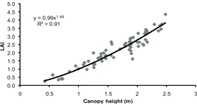
Development of the model to estimate the LAI The correlations between LAI and canopy height were analysed (Figure 3), as well as between LAI and PRV (Figure 4), the results being signifi cant in both cases at a confi dence level of 95 %, with determination coeffi cients (R2) of 0.91 and 0.94, respectively. Easily
measured parameters in the plant mass of the tomato crop permit the estimation of an index as complex as LAI. This is because the normal development of the to-mato plant has regular node distribution and leaf develop-ment. However, the LAI has a closer relationship with PRV than with canopy height, since the PRV value, apart from taking into account canopy height also takes into account the development of the leaves in an indirect way from the width of the vegetation. The model relating LAI with PRV corresponds to a power equation, similar to
Table 4 – Working parameters for the applications.
Season Applications PRV Conventional application Estimated application
Pressure Speed VCONb V
ESTc Pressure Speed VFd
m3 ha–1 kPa m s–1 --- L ha–1 --- kPa m s–1 L ha–1
Spring-summer 2011
1 6442.09 1185 1.22 1277.89 808.00 758 1.58 790.76
2 6314.20 1179 1.25 1246.34 788.00 653 1.42 817.16
3 5978.60 1178 1.36 1149.42 736.00 593 1.42 779.88
4 6467.59 1159 1.20 1284.20 812.00 604 1.29 862.50
Autumn-winter 2011/12
1 7047.46 1188 1.10 1426.19 904.00 581 1.15 954.37
2 8221.40 1211 0.91 1732.26 1096.00 623 1.01 1121.64
3 8532.00 1201 0.87 1814.29 1148.00 592 0.95 1168.09
4 8674.40 1235 0.86 1852.16 1172.00 654 0.99 1173.34
aPlant Row Volume V CON;
bapplication rate calculated with the farmer’s criteria; cV
EST, application rate calculated with Eq. 6; dV
F, application rate calculated under fi eld
conditions.
Figure 2 – Greenhouse plant with the compartmentalization in experimental blocks and plots.
y = 0.99x1.49
R² = 0.91
0.0 0.5 1.0 1.5 2.0 2.5 3.0 3.5 4.0 4.5 5.0
0 0.5 1 1.5 2 2.5 3
LAI
Canopy height (m)
the model reported by Siegfried et al. (2007)to relate LAI and VRV (Vine Row Volume) in grapevine.
To determine which of the models offered the best estimation of the LAI, a calculation was made of the Relative Standard Error (RSE) from the data (11 data in total) of a series of plants sampled (Table 2), which were not included in the models developed. For each model used to estimate LAI, Table 5 shows the PRESS, the RSE, and the equation. These models to estimate LAI were validated only for greenhouse tomato crops with normal vegetative development (internodes of c. 5-16 cm, depending on the growth stage), cultivated with adequate irrigation and nutrients as well as proper management (leaf thinning, branch thinning, and tip pinching).
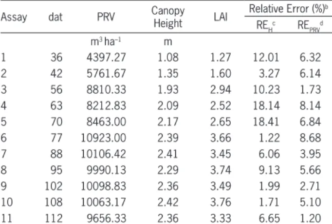
The analysis of the LAI values estimated for each datum used for validation (Table 6) indicated that the model based on the canopy height had greater relative errors between tests 3 and 5, with values higher than 10 %. This was because just at 56 dat (days after transplanting) the plants were leaf thinned. The thinning, i.e. clipping off the lower leafs of the plants, decreased the leaf sur-face area, reducing the LAI by 14 % from assay 3 to 4. However, leaf thinning did not lower the canopy height, which between assay 3 and 4 increased 8 %, resulting in errors of more than the 10 % indicated above. On the other hand, the canopy height was shortened when tip pinched, which consisted of removing the tip of the main stem, limiting plant growth. Tip pinching was performed at 88 dat, although this operation did not lead to major errors in estimating the LAI with the canopy height, (all were under 10 %) because the loss in leaf area was mi-nor, since new leaves were located at the tip of the stem, representing minor surface-area development.
For the model used to estimate LAI based on the PRV, all the errors were lower than 9 % (Table 6), even after leaf thinning and tip pinching, which prompted major changes in plant architecture. Nevertheless, major errors (c. 8 %) also arose just after leaf thinning.
The two models enabled a good estimation of the LAI with relative standard errors lower than 9 %. Never-theless, the model that offered the best estimation of the LAI was the one based on the PRV with a RSE of 5.44
%. Taking into account the PRV-LAI relationship, Eq. 5 enabled the volume application rate to be determined as a function of PRV (Eq. 6.):
V = 7.10–3 . d
V . PRV
1.25/ (6)
Evaluation of the method to determine the volume rate for spraying
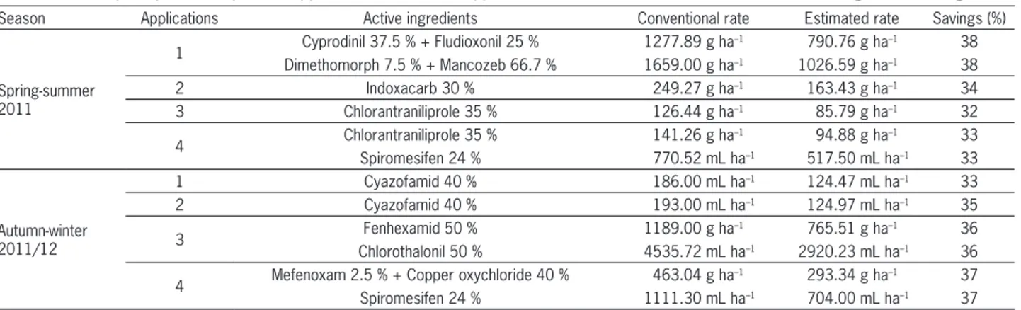
An evaluation was made of the plant protection achieved over two seasons (spring-summer 2011, au-tumn-winter 2011-12). Table 7 lists the products applied in each season and the dose applied for the CON and EST strategies, calculated on the basis of the volume shown in Table 4 for each strategy. The aim of these assays was to compare two strategies to calculate the application volumes: the CON rate, calculated with the criteria of the farmer (VCON), and the EST rate, calcu-lated from the PRV using Eq. 6 (VEST). For this, the yield corresponding to each treatment was compared for pos-sible differences.
Table 7 shows the percentage of savings of the chemical when Eq. 6 was used to estimate the volume application rate. The savings in both seasons consistently exceeded 30 %, with mean values of 34.39 % and 35.15 % in the fi rst and second season, respectively.
In terms of yield, Table 8 shows the mean values calculated in the areas where each control strategy was evaluated. The two strategies gave similar yield in both seasons. There were no differences (p < 0.05) with
y = 3.5·10–5·x1.25
R2= 0.94
0.0 0.5 1.0 1.5 2.0 2.5 3.0 3.5 4.0 4.5 5.0
0 2000 4000 6000 8000 10000 12000
LAI
PRV (m3ha–1)
Figure 4 – Plant row volume (PRV)- Leaf area index (LAI) regression curve.
Table 5 – Values of the prediction residual sum of squares (PRESS), the relative standard error (RSE) and equation for each model.
Models to estimate LAI PRESS RSE
(%) Model equation R2 Based on the canopy
height 0.78 8.73 LAI = 0.99·(H)1.49 0.91 Based on PRV 0.30 5.44 LAI = 0. 35·10–4·(PRV)1.25 0.94
Table 6 – Relative errors in estimating the leaf area index (LAI) with each of the models.
Assay dat PRV Canopy Height LAI
Relative Error (%)b
REHc RE PRV
d
m3 ha–1 m
1 36 4397.27 1.08 1.27 12.01 6.32
2 42 5761.67 1.35 1.60 3.27 6.14
3 56 8810.33 1.93 2.94 10.23 1.73
4 63 8212.83 2.09 2.52 18.14 8.14
5 70 8463.00 2.17 2.65 18.41 6.84
6 77 10923.00 2.39 3.66 1.22 8.68
7 88 10106.42 2.41 3.45 6.06 3.95
8 95 9990.13 2.29 3.74 9.13 5.66
9 102 10098.83 2.36 3.49 1.99 2.71 10 108 10063.17 2.42 3.76 1.71 5.10 11 112 9656.33 2.36 3.33 6.65 1.20
aPlant Row Volume; bRelative error (%) = |LAI-LÂI|/LAI·100; cRelative error with
Table 7 – List of plant protection product applied in each season. Applied dose for the conventional and estimated strategies and savings. Season Applications Active ingredients Conventional rate Estimated rate Savings (%)
Spring-summer 2011
1 Cyprodinil 37.5 % + Fludioxonil 25 % 1277.89 g ha
–1 790.76 g ha–1 38
Dimethomorph 7.5 % + Mancozeb 66.7 % 1659.00 g ha–1 1026.59 g ha–1 38
2 Indoxacarb 30 % 249.27 g ha–1 163.43 g ha–1 34
3 Chlorantraniliprole 35 % 126.44 g ha–1 85.79 g ha–1 32
4 Chlorantraniliprole 35 % 141.26 g ha
–1 94.88 g ha–1 33
Spiromesifen 24 % 770.52 mL ha–1 517.50 mL ha–1 33
Autumn-winter 2011/12
1 Cyazofamid 40 % 186.00 mL ha–1 124.47 mL ha–1 33
2 Cyazofamid 40 % 193.00 mL ha–1 124.97 mL ha–1 35
3 Fenhexamid 50 % 1189.00 g ha
–1 765.51 g ha–1 36
Chlorothalonil 50 % 4535.72 mL ha–1 2920.23 mL ha–1 36
4 Mefenoxam 2.5 % + Copper oxychloride 40 % 463.04 g ha
–1 293.34 g ha–1 37
Spiromesifen 24 % 1111.30 mL ha–1 704.00 mL ha–1 37
Table 8 – Commercial yield in each season.
Application strategy spring-summer 2011 autumn-winter 2011/12 --- kg m–2
---Conventional application rate 8.8 9.0 Estimated application rate 8.9 8.9
respect to the main factors (control strategy, block and greenhouse) or between their interactions. The similarity of the yield in both treatments, VCON and VEST, means that the crop was suitably protected despite the decrease in volume applied. If the volume application rates in VEST had not been enough to control the pest attack, there would have been reduction in the yield.
Conclusions
The model that offered the best results was based on the PRV. The errors in estimating the LAI were rela-tively low even after leaf thinning and tip pinching, which alter the plant architecture. The estimation of LAI from the PRV defi ned a strategy by which volume application rate could be matched to the characteristics of the crop. This strategy presented satisfactory results, providing a reduction of more than 30 % with respect to the conventional volume application rate.
Acknowledgements
This study was supported by grant P07-AGR-02995 from CICE-Junta de Andalucía (Spain), co-fi nanced with FEDER funds of the European Union.
References
Barani, A.; Franchi, A.; Bugiani, R.; Montermini, A. 2008. Effi cacy of unit canopy row spraying system for control of European vine moth (Lobesia botrana) in vineyards. Available at: http://www. cigrjournal.org/index.php/Ejounral/article/viewFile/1244/1102 [Accessed Nov. 28, 2012].
Beulke, S.; van Beinum, W.; Glass, R.; van Os, E.; Holterman, H.; Sapounas, A.; Voogt, W.; van de Zande, J.; de Zwart, F.; Garratt, J. 2011. Estimation/calculation of emissions of plant protection products from protected crops (greenhouses and cultivations grown under cover) to support the development of risk assessment methodology under Regulation (EC) n° 1107/2009 and Council Directive 91/414/EEC. European Food Safety Authority (EFSA). Available at: http://www.efsa.europa. eu/en/supporting/pub/151e.htm [Accessed Nov 28, 2012]. Byers, R.E.; Hickey, K.D.; Hill, C.H. 1971. Base gallonage per
acre. Virginia Fruit 60: 19-23.
Cerruto, E.; Emma, G.; Manetto, G. 2009a. Spray applications to tomato plants in greenhouses. I. Effect of walking direction. Journal of Agricultural Engineering 3: 41-48.
Cerruto, E.; Emma, G.; Manetto, G. 2009b. Spray applications to tomato plants in greenhouses. II. Effect of spray lance type. Journal of Agricultural Engineering 3: 49-56.
Dammer, K.; Wollny, J.; Giebel, A. 2008. Estimation of the Leaf Area Index in cereal crops for variable rate fungicide spraying. European Journal of Agronomy 28: 351-360.
Furness, G.O.; Magarey, P.A.; Miller, P.M.; Drew, H.J. 1998. Fruit tree and vine sprayer calibration based on canopy size and length of row: Unit canopy row method. Crop Protection 17: 639-644.
Gil, E.; Escolà, A. 2009. Design of a decision support method to determine volume rate for vineyard spraying. Applied Engineering in Agriculture 25: 145-151.
Gil, E.; Escolà, A.; Rosell, J.R.; Planas, S.; Val, L. 2007. Variable rate application of plant protection products in vineyard using ultrasonic sensors. Crop Protection 26: 1287-1297.
Giles, D.K.; Delwiche, M.J.; Dodd, R.B. 1989. Sprayer control by sensing orchard crop characteristics: Orchard architecture and spray liquid savings. Journal of Agricultural Engineering Research 43: 271-289.
Koch, H. 2007. How to achieve conformity with the dose expression and sprayer function in high crops. Pfl anzenschutz-Nachrichten Bayer 60/2001 1: 71-84.
Rüegg, J.; Viret, O.; Raisigl, U. 1999. Adaptation of spray dosage in stone-fruit orchards on the basis of the tree row volume. Bulletin OEPP/EPPO 29: 103-110.
Sánchez-Hermosilla, J.; Rincón, V.J.; Páez, F.; Agüera, F.; Carvajal, F. 2011. Field evaluation of a self-propelled sprayer and effects of the application rate on spray deposition and losses to the ground in greenhouse tomato crops. Pest Management Science 67: 942-947.
Sánchez-Hermosilla, J.; Rincón, V.J.; Páez, F.; Fernández, M. 2012. Comparative spray deposits by manually pulled trolley sprayer and a spray gun in greenhouse tomato crops. Crop Protection 31: 119-124.
Siegfried, W.; Viret, O.; Huber, B.; Wohlhauser, R. 2007. Dosage of plant protection products adapted to leaf area index in viticulture. Crop Protection 26: 73-82.
Sutton, T.B.; Unrath, C.R. 1988. Evaluation of the tree-row-volume model for full-season pesticide application on apples. Plant Disease 72: 629-632.