doi: 10.1590/0101-7438.2016.036.02.0321
A COMPARATIVE STUDY BETWEEN ARTIFICIAL NEURAL NETWORK AND SUPPORT VECTOR MACHINE FOR ACUTE
CORONARY SYNDROME PROGNOSIS
Rodrigo Abrunhosa Collazo
1, Leonardo Antonio Monteiro Pessˆoa
1*,
Laura Bahiense
2, Bas´ılio de Braganc¸a Pereira
2,4,
Am´alia Faria dos Reis
3and Nelson Souza e Silva
4Received October 31, 2015 / Accepted July 13, 2016
ABSTRACT.Despite medical advances, mortality due to acute coronary syndrome remains high. For this reason, it is important to identify the most critical factors for predicting the risk of death in patients hospitalized with this disease. To improve medical decisions, it is also helpful to construct models that enable us to represent how the main driving factors relate to patient outcomes. In this study, we compare the capability of Artificial Neural Network (ANN) and Support Vector Machine (SVM) models to distinguish between patients hospitalized with acute coronary syndrome who have low or high risk of death. Input variables are selected using the wrapper approach associated with a mutual information filter and two new proposed filters based on Euclidean distance. Because of missing data, the use of a filter is an important step in increasing the size of the usable data set and maximizing the performance of the classification models. The computational results indicate that the SVM model performs better. The most relevant input variables are age, any previous revascularization, and creatinine, regardless of the classification algorithms and filters used. However, the Euclidean filters also identify a second important group of input variables: age, creatinine and systemic arterial hypertension.
Keywords: acute coronary syndrome, heart disease, variable selection, support vector machine, artificial neural network, filter, Euclidean distance.
*Corresponding author.
1Centro de An´alises de Sistemas Navais – CASNAV, Rio de Janeiro, RJ, Brasil.
2Instituto Alberto Luiz Coimbra de P´os-Graduac¸˜ao e Pesquisa em Engenharia – COPPE, Universidade Federal do Rio de Janeiro – UFRJ, Rio de Janeiro, RJ, Brasil.
3Hospital Universit´ario Antonio Pedro, Universidade Federal Fluminense – UFF, Niter´oi, RJ, Brasil.
4Faculdade de Medicina e Hospital Universit´ario Clementino Fraga Filho, Universidade Federal do Rio de Janeiro – UFRJ, Rio de Janeiro, RJ, Brasil.
1 INTRODUCTION
Cardiovascular diseases, including cerebrovascular and ischemic heart diseases, are major causes of death worldwide and the main cause of death in Brazil. In particular, Acute Coronary Syn-dromes (ACSs) are prominent in maintaining a high mortality rate despite recent therapeutic advances. These syndromes are characterized by total or partial occlusion of the coronary artery. This leads to ischemia and/or necrosis of the myocardial area irrigated by the coronary artery, following the rupture of an unstable coronary plaque. ACSs include acute myocardial infarction (with and without ST-segment elevation) and unstable angina.
ACSs may result from the interaction of environmental, clinical, genetic, and socio-cultural fac-tors. To obtain a reliable and effective clinical prognosis of patients with an ACS it is thus vi-tal to identify the most important variables. This is also a critical step in developing medical decision-supporting tools associated with clinical and laboratory procedures in order to reduce the mortality rate and financial costs.
In this multi-factorial causal context, non-linear modelling methods have the required flexibil-ity to construct classifiers with good predictive performance. Artificial Neural Network (ANN) (Bishop, 1995) and Support Vector Machine (SVM) (Boser et al., 1992; Cortes & Vapnik, 1995) are well-established examples of these types of models. They have been used in several stud-ies for diagnosis and prognosis of coronary heart diseases; see e.g. U˘guz (2012); Khemphila & Boonjing (2011); Sengur (2012); C¸ omak & Arslan (2012); Kohli & Verma (2011). Comparative analyses between the predictive power of both models in this domain have also been published and are briefly reviewed below since they are the focus of this work.
Berikol et al. (2016) tested the accuracy of four different classifiers (SVM, ANN, Naive Bayes, logistic regression) for ACS diagnosis using a data set with 228 patients (99 with ACS and 129 without ACS) and 8 variables. The SVM presented higher accuracy (99%) than ANN (90%), Naive Bayes (89%) and logistic regression (91%). Kumari & Godara (2011) compared four clas-sification techniques (RIPPER, Decision Tree, ANN, and SVM) in terms of their capability to predict the diagnosis of cardiovascular disease in general. They used a data set with 296 pa-tients and 14 input variables. No preprocessing for input variable selection was performed in this study, and the results indicated that the SVM model was superior. Xing et al. (2007) assessed the performance of Decision Tree, ANN and SVM to predict the 6-month survival of patients with coronary heart disease using a data set with 1,000 individuals. The results regarding the accuracy of the classifiers employed were very similar: 92.1% for SVM, 91.0% for ANN, and 89.6% for the Decision Tree.
techniques. The performance of the SVM algorithm was compared to that of a previous study using an ANN (Turkoglu et al., 2002). The results indicated the superiority of the ANN in terms of sensitivity and specificity. However the authors recommended using the SVM model because of the shorter training times and greater stability in converging to the solution.
Despite it being well-known that the main drivers underlying the cardiovascular diseases can substantially vary from country to country there is a lack of similar comparative studies focused particularly on the Brazilian population. To the best of our knowledge, this is not restricted to the public health and medical settings but is also pervasive over the whole spectrum of Brazilian challenges. This happens regardless of the existence of an extensive literature in Soft Operational Research that highlights the cross fertilisation benefits between different methodologies. For a work that explores the use of multi-methodologies for understanding a real-world process of a Brazilian hospital, see Pessˆoa et al. (2015).
We have also noted that many works have recently explored the synergistic links between Oper-ational Research (OR) and Artificial Intelligence (AI) (Holsapple et al., 1994; Brown & White, 2012; Gomes, 2001). In particular, the interplay between OR and AI with regard to decision support systems and optimization are discussed in Wojewnik & Kuszewski (2010) and Bennett (2006), respectively. For an interesting study that compares the capability of ANN, SVM and genetic algorithm to predict the Brazilian Power Quality, see G´oes et al. (2015).
In this study we aim at reducing this gap in applied health studies and exploring the links between OR and AI on behalf of the Brazilian population. Our objective is to compare the predictive power of the ANN and SVM models in terms of classifying the risk of death (high or low) in Brazilian patients admitted with ACSs. This also differs from previous studies whose aim is often thediagnosis of cardiovascular diseasesinstead of theintra-hospital prognosis. In this sense our work comes closer to the survival study of Xing et al. (2007). However those authors were interested in thepost-hospital prognosissince they defined survival as a patient being alive after 6-months of a positive diagnosis of coronary heart disease.
Here the data set has clinical, genetic and socio-environmental variables. However, the use of variables that are not relevant for predicting patient outcomes can disrupt the training and com-promise the generalization power of the model. Furthermore, a model with all variables forces us to discard a large number of individuals because of missing data. The number of possible vari-able sets to be examined grows exponentially with the number of varivari-ables. So, a large number of variables – as is the case here – implies a great computational cost as regards time and memory.
In practice, one common way to circumvent this issue is to adopt a heuristic variable selection method that allows us to identify quickly a few but potentially promising variable sets. For this purpose, we first order the input variables using a filter. Next each classification algorithm is used independently to select the most relevant set of input variables.
process, which requires a considerable amount of human, material and financial resources (Kononenko, 2001). Also note that our emphasis on variable selection is another point that con-trasts with the reviewed literature whose works do not often aim at identifying the most critical variables for the diagnosis of heart disease.
The comparative study between ANN and SVM algorithms are based on the well-established Mutual Information Feature Selector under Uniform information distribution (MIFS-U) criterion (Kwak & Choi, 2002; Gonc¸alves & Macrini, 2011). To verify the robustness of the results with regard to this mutual information filter we retrain the classification algorithm with better perfor-mance using the orders of variables provided by two new filters based on Euclidean distance. The development of these Euclidean filters is our main methodological contribution.
We performed logistic regression analyses, both with and without first-order multiplicative interaction of the input variables selected in the preprocessing filter step. The sensitivity results for all tested variable sets were under 10%, as already expected because of the very small ratio of death events per variable (Concato et al., 1995; Peduzzi et al., 1995, 1996). For brevity, we excluded experiments using logistic regression from the scope of this study.
This article is organized as follows. In the next section, we review the variable selection methods and the SVM and ANN algorithms and introduce our Euclidean filters. In Section 3, the data set used in the experiments is described. In Section 4, we discuss the results of the computational experiments, which includes the comparative experiments and the corresponding robustness anal-ysis. In the Conclusion, final remarks are presented and future works outlined.
2 DATA MINING TECHNIQUES
The variable selection methods and the ANN and SVM models employed in this study are briefly discussed in this section.
2.1 Variable Selection Method
To construct efficient classifiers, variable selection is an important step for the following reasons (Salappa et al., 2007; Guyon & Elisseeff, 2003; Saeys et al., 2007):
1. to avoid overfitting, to reduce noise, and (through this process) to improve the predictive power of the classifier;
2. to obtain models with reduced computational cost, both in terms of the processing time and the memory requirements; and
3. to directly elucidate the underlying process responsible for generating the data.
The variable selection methods can be grouped into three broad classes: a filter, a wrapper, and an embedded method (Guyon & Elisseeff, 2003; Saeys et al., 2007; Blum & Langley, 1997). Filters correspond to a preprocessing technique that selects input variables before training the classification algorithm. The advantages of filters are the ease and speed of implementation, whilst their main disadvantage is that they ignore the interaction with the classifier.
Wrappers use the classification algorithms as black boxes to assess the predictive power of sub-sets of input variables. These subsub-sets are normally built either randomly or through a heuristic procedure. Finally, embedded methods incorporate the selection method into the classifier train-ing process. The main advantage of these two latter methods is the fact that they interact with the classification algorithm. However this interaction also constitutes the source of their drawbacks, namely greater computational cost (i.e., time and memory) and dependency on the classification algorithm itself.
Our approach combines a wrapper method and a filter. This enables us to take advantage of the benefits offered by these two methods and at the same time to minimize their deficiencies. First, to compare the ANN and the SVM algorithm we use the MIFS-U filter. Via a greedy strategy this filter provides us with an order of input variables based on the degree of mutual information between input variables and the response variable. The density distributions of the variables are approximated by their histograms, and it is assumed that the information contained in these variables is uniformly distributed. In the second experiment, to explore the robustness of the results we use two new filters based on Euclidean distance. These filters are discussed in Section 2.2.
The order of variables is used as an input for the wrapper approach. We adopt the sequential forward-selection strategy, where the classification algorithm (ANN or SVM) evaluates each nested subset of variables until the classification error begins to increase. In other words, the classification algorithm evaluates the subset with thek+1 first variables if and only if the subset with the firstkvariables yields a classification error below what was obtained from the subset with thek−1 first variables. However, the variable selection is not interrupted until the minimum value ofkequal to six is reached.
Classification errors are assessed using the following concepts:
Accuracy (a) This is the probability of correctly predicting the outcome.
Sensitivity (x) This is the probability of correctly predicting the high death risk.
Specificity (y) This is the probability of correctly predicting the low death risk.
The Pearson correlation coefficient (PCC) is used to assess the performance of the classifiers. This coefficient provides a balance between the concepts of sensitivity and specificity. The value of PCC ranges from−1 (total disagreement) to 1 (total agreement), and a zero value represents totally random predictions (Baldi et al., 2000).
set containsL−1 individuals and the test sample consists of the excluded individual, which is different in each training. In the end, the probabilities are estimated by
ˆ
a= T
L, xˆ= TP LP
, yˆ= TN
LN
, (1)
whereT is the total number of correct predictions obtained by the classifier for a given data set;
TP andLPare, respectively, the number of positive data points that are correctly classified and
the total number of positive data points; andTNandLNare, respectively, the number of negative
data points that are correctly classified and the total number of negative data points.
2.2 New Euclidean Filters
Here two ordering criteria for the input variables are developed using Euclidean distance. The only source of information for these criteria is the data themselves. This is because even among medical specialists there is no established consensus regarding the absolute and/or relative im-portance of each variable to some given ACS prognosis.
Initially, we briefly analyze the ordering criterion developed in a previous study by Chen et al. (2009). To minimize text and avoid repeatedly referencing this article, we refer to this particular criterion as CZCL (the initials of its authors’ names). Also letT = {(x1,y1), . . . , (xl,yl)}be a
sample withlindividuals, wherexi =(xi1, . . . ,xin)and wherexi j is the value of a variable j
for an individuali andyi ∈ {−1,1}is the value of the response variable for an individuali.
2.2.1 CZCL Criterion
The CZCL criterion is based on two hypotheses:
1. If small changes of an input variable correspond to large variations in the response variable, the input variable is relevant.
2. If small changes of an input variable correspond to small variations in a response variable, then the input variable is unimportant.
This criterion orders the variables according to the following score:
Fk =g1·VAk+g2·Sk, (2)
where VAk is a score assigned to the kt h variable by domain experts and Sk is an objective
score for thekt h variable. The positive parametersg1andg2set the balance between domain knowledge and data. The scoreSkis formally defined by
Sk=
maxk∈{1,...,n}(Tk)−Tk
maxk∈{1,...,n}(Tk)−mink∈{1,...,n}(Tk)
, (3)
where:
Tk = l
r=1 l
s=1,s=r
d(yr,ys)
dk′(xr,xs)
dk′(xr,xs)= [d2(xr,xs)−dk2(xr,xs)] 1
2 (5)
d2(xr,xs)= n
i=1
(xri−xsi)2 (6)
dk2(xr,xs)=(xrk−xsk)2 (7) d(yr,ys)= |yr−ys| (8)
Note thatSkcorresponds to a normalization ofTkin order to use the same scale for the termsTk
andVAk. Because our goal is to use only the data, we can drop the termVAkand the parameters g1andg2from Equation 2 . Thus, there is no need to compute the value ofSkand we can order
the variables using the score given by:
TkC Z C L = Tk maxk∈{1,n}(Tk)
(9)
The hypothesises above then imply that a relevant variable has a low scoreTC Z C L.
Acording to Chen et al. (2009), the CZCL criterion has the following advantages:
1. It takes into account the relations between input and output variables when selecting which variables are more relevant.
2. It uses the primitive input variables instead of some transformation thereof, as is done in principal component analysis.
3. It does not require a large number of data points.
4. It does not require the data to conform to any statistical distribution.
5. It can capture non-linear relations between input and output variables.
6. It is simple to implement and has low computational cost.
2.2.2 Disagreement Criterion
Since in this study the response variable has only two categories, we only need to calculateTk
(Equation 4) for pairs of individuals who have distinct outcomes. We then have that
Tk =
r|y=1
s|y=−1
|yr−ys| dk′(xr,xs)
=2
r|y=1
s|y=−1 1
dk′(xr,xs)
. (10)
Now note that there is no loss of information if we re-expressTk by:
Tk∗= r|y=1
s|y=−1
[dk′(xr,xs)]2=
r|y=1
s|y=−1
Because the term d2(xr,xs)is present in the computation of all variables, its omission does
not affect the relative order of the variables whilst also achieving a score that is more sensitive to the main term dk2(xr,xs). Implementing this change, we can then order variables using a
disagreement score given by
TkD= (T ′ k)
maxk∈{1,,n}(Tk′)
, (12)
where
Tk′ = r|y=1
s|y=−1
dk2(xr,xs). (13)
Keeping valid both hypotheses assumed for the CZCL criterion, the relevance of thekt hvariable increases as the value ofTkDdecreases.
The disagreement criterion has two additional advantages compared to the CZCL criterion:
1. It is more sensitive to the main quantity of interestdk2(xr,xs).
2. It has lower computational cost.
2.2.3 Inverse Criteria
The scores TkC Z C L andTkD are based on the Euclidian distance between the input variablek
in two different individuals. Because of the sensitivity hypotheses, their corresponding criteria described above select those variables for which the summed distances are small. However, it is also reasonable to assume the converse of this condition: input variables corresponding to large distances are more able to distinguish between two possible outcomes (Dash & Liu, 1997). Based on this new hypothesis, those variables with large scoresTkC Z C L orTkDare more relevant. This assumption yielded criteria called the inverse criteria. Therefore, the inverse CZCL criterion and the inverse disagreement criterion select input variables that have, respectively, the highest scores
TkC Z C L andTkD.
2.3 Artificial Neural Network (ANN) Model
The specific type of ANN (Bishop, 1995; Haykin, 1999; Teixeira J´unior et al., 2015) used in this study is a three-layer feed-forward ANN. The input layer haskinput neurons and one bias neuron, wherekcorresponds to the number of input variables included in the model. The hidden layer is initially composed of 10 hidden neurons and one bias neuron. Finally, the output layer has one output neuron. The hyperbolic tangent is adopted as an activation function for the hidden layer, whereas a linear function is assigned to the output layer. This structure is justified by its simplicity. Moreover, if it is assumed there are non-identical data in distinct categories, three-layer neural classifiers are universal classifiers (Young & Downs, 1998).
To avoid over-fitting we adopt the Bayesian regularization algorithm (MacKay, 1992). In this framework, the ANN weights and biases are assumed to be random variables. The regularization parameters are the unknown variances associated with these distributions and can be estimated through adequate statistical techniques. The result is the minimization of a function that is a linear combination of the quadratic errors and the weights of the hidden and output layers. Bayesian regularization requires the Hessian matrix to be computed, which implies using the Levenberg-Marquardt algorithm (Nocedal & Wright, 2006). Ultimately, this structure enables us to select the smallest set of neurons in the hidden layer that provides the best optimization of the ANN.
2.4 Support Vector Machine (SVM)
Solving a convex quadratic problem, the SVM model (Boser et al., 1992; Cortes & Vapnik, 1995; Suykens et al., 2010; Scholkopf & Smola, 2001) selects a hyperplane that minimizes structural risk. The minimization of structural risk (Vapnik, 2006) establishes a compromise between the complexity of the decision function space and the ability to fit the model to the training data set (empirical risk). This process guarantees a good generalization power for the trained classifier, i.e., a strong propensity to correctly predict the outcome of an individual out of the training sample.
When associated with a kernel function, the SVM model allows non-linear classifiers to be built by implicitly mapping the initial data into a space of higher dimension than the original one. In this case, the linear classifier obtained in a higher-dimension space corresponds to a non-linear classifier in the original space.
Here we use theν-SVM (Scholkopf & Smola, 2001; Chen et al., 2005; Scholkopf et al., 2000). This classifier was initially conceived to recognize two types of patterns and was subsequently extended to multi-class and regression problems. Inν-SVM training, it is necessary to adjust the parameter, which represents the upper limit for the fraction of training errors and the lower limit for the fraction of support vectors. These interpretations of theν parameter simplify its calibration. The kernel function adopted in this study is the hyperbolic tangent since the goal is to compare the SVM and ANN classifiers (Karatzoglou et al., 2006).
To train the classifier, we use the Sequential Minimal Optimization (SMO) algorithm (Platt et al., 1999). This algorithm analytically determines the global solution, optimizing at each itera-tion only two Lagrangian multipliers from the convex quadratic problem corresponding to the model’s mathematical formulation. The SMO algorithm requires minimal computational mem-ory resources and is extremely fast because it performs only a limited number of very simple operations.
3 EXPERIMENTAL DESIGN
The data set contains 28 explanatory variables, which are classified into five categories: social and anthropometric variables; variables related to previous cardiovascular history; clinical and laboratory variables concerning hospital admission; diagnosis variables; and genetic variables. The response variable is the occurrence of in-hospital death. These variables are described in Appendix A, which includes information regarding the measurement scales and lists the abbre-viation used for each variable.
4 RESULTS AND DISCUSSION
The MIFS-U filter and the ANN models are implemented using the MATLAB software, version 7.0. The Euclidean filter andν-SVM models are run in the R software, version 2.7.0, using the kernlab package. To avoid scale issues, the data are normalized.
4.1 Comparison between ANN and SVM using the MIFS-U filter
The MIFS-U criterion is used two times consecutively. Initially the filter is applied to a sample with 264 individuals (17 deaths and 247 survivals), for whom data regarding the response variable and all 28 input variables are available. The order obtained for the 28 input variables with respect to the response variable death is shown in Table 1.
Table 1–First phase of the MIFS-U filter
Position Variable Position Variable
1 Age 15 TT genotype
2 APR 16 Gender
3 Creatinine 17 HDL cholesterol
4 DD genotype 18 MT genotype
5 E2E2 genotype 19 II genotype
6 E4E4 genotype 20 Smoking
7 BMI 21 Total cholesterol
8 E2E3 genotype 22 ACS
9 SAH 23 DI genotype
10 E3E4 genotype 24 Killip
11 E2E4 genotype 25 Triglyceride
12 Diabetes mellitus 26 PMI
13 MM genotype 27 Education level
14 E3E3 genotype 28 Heart rate
Table 2–Second phase of the MIFS-U filter.
Position Variable Change Position Variable Change
1 Age 0 9 E3E4 genotype –1
2 APR 0 10 Diabetes mellitus –2
3 Creatinine 0 11 E2E4 genotype 0
4 BMI –3 12 E2E3 genotype +4
5 DD genotype +1 13 MM genotype 0
6 E4E4 genotype 0 14 SAH +5
7 E2E2 genotype +2 15 TT genotype 0
8 Gender –8 16 E3E3 genotype +2
The results show that the three top-ranking variables remain unchanged in both orders of vari-ables. Note that the variables Age, Any Previous Revascularization (APR), Creatinine, Body Mass Index (BMI), DD, and E2E2 and E4E4 Genotypes are the seven variables holding the most combined mutual information regarding the outcome of interest. Also observe that seven variables (Age; Any Previous Revascularization; Creatinine; and E2E4, E4E4, MM, and TT Genotypes) do not change their ranks between each filter pass, and two variables (DD and E3E4 Genotypes) change by only one position. The variables E2E2 Genotype, E3E3 Genotype and Diabetes Mellitus shift their orders by only two positions whilst the variable Body Mass Index shifts its rank by three positions. In contrast, the variables with the greatest changes in terms of positions are E2E3 Genotype (four positions), Systemic Arterial Hypertension (SAH) (five positions), and Gender (eight positions). The results can therefore be considered stable since the greatest changes in the ordering only appear after the eighth position.
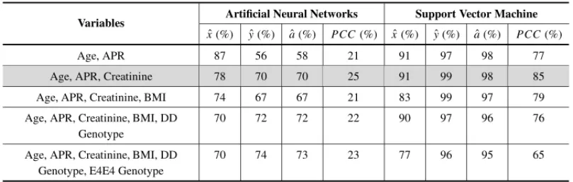
Table 3 summarizes the results for the ANN and SVM models trained using the sample with 351 individuals for all sets of variables. Classifiers built with the three top-ranking variables according to the MIFS-U filter (Age, Any Previous Revascularization, and Creatinine) yielded the best results in both models. Thus, the best classifiers are obtained from the information contained in an integer variable (Age), a categorical variable (Any Previous Revascularization), and a continuous variable (Creatinine).
Table 3–Results from the ANN and SVM models.
Variables Artificial Neural Networks Support Vector Machine ˆ
x(%) yˆ(%) aˆ(%) PCC(%) xˆ(%) ˆy(%) aˆ(%) PCC(%)
Age, APR 87 56 58 21 91 97 98 77
Age, APR, Creatinine 78 70 70 25 91 99 98 85
Age, APR, Creatinine, BMI 74 67 67 21 83 99 97 79
Age, APR, Creatinine, BMI, DD Genotype
70 72 72 22 90 97 96 76
Age, APR, Creatinine, BMI, DD Genotype, E4E4 Genotype
The fact that genetic and diagnostic variables do not contribute to the construction of the optimal classifiers stands out. In the case of the ANN classifier, an increased number of input variables tends to decrease sensitivity and to increase specificity. Therefore, the choice of the first three variables represents a compromise between these two concepts, as determined using Pearson cor-relation coefficient. Note that the SVM model with those three variables has superior predictive power compared to any ANN model trained.
4.2 Robustness Analysis using SVM and Euclidean Filters
To verify in which extension the filter biased the wrapper variable selection we revisit the data set using the Euclidean filter a single time. For brevity, we focus on the SVM model since it clearly outperformed the ANN model previously.
To assess the importance of genetic variables for the prognosis of ACS here we adopt their parametrisation in terms of allele instead of genotype. For example, take the E Apolipprotein
gene polymorphism. In the first experiment, we considered six input variables corresponding its six genotypes X Y, where X,Y = E2,E3,E4 were their possible alleles. Now we have only three binary variables E2,E3,E4 corresponding to the three allele associated with this polymorphism. Observe that this new definition does not cause any loss of information. We also include three additional variables: time elapsed before first medical attention, family history of coronary arterial disease and physical activity. The first two variables were excluded from the first experiment because they are not directly associated with each sampled individual. The last variable was initially omitted because we assumed that the variables Body Mass Index and physical activity capture similar information. Appendix B describes these three variables and the re-parametrised genetic variables.
Table 4–CZCL Criterion (Inverse CZCL Criterion).
Position Variable TC Z C L
K Position Variable TKC Z C L
1 (26) APR 0.98404 14 (13) FHD 0.99172
2 (25) E3 allele 0.98532 15 (12) Triglyceride 0.99182
3 (24) TFM 0.98588 16 (11) Physical Activity 0.99253
4 (23) PMI 0.98786 17 (10) ACS 0.99314
5 (22) E2 allele 0.98795 18 (9) Gender 0.99383
6 (21) SAH 0.98847 19 (8) Diabetes mellitus 0.99402
7 (20) E4 allele 0.98925 20 (7) Education Level 0.99435
8 (19) I allele 0.98981 21 (6) Killip 0.99442
9 (18) T allele 0.999012 22 (5) Smoking 0.99517
10 (17) BMI 0.999018 23 (4) HDL Cholesterol 0.99532
11 (16) D allele 0.99054 24 (3) Age 0.99862
12 (15) M allele 0.99091 25 (2) Heart Rate 0.99873
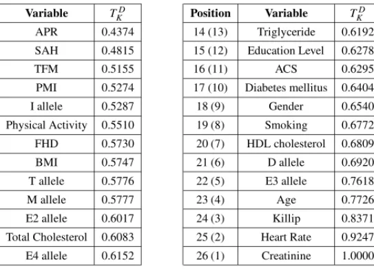
The four criteria (CZCL criterion, inverse CZCL criterion, disagreement criterion and inverse disagreement criterion) are applied to a complete sample with 226 individuals, of whom 16 had fatal outcomes. Tables 4 and 5 show the orders of variables given, respectively, byTkC Z C L and
TkD. As discussed in Section 2.2, the scoreTkDprovides a more well-defined classification of the input variables than the scoreTkC Z C L: the distance between the first and last variables usingTkD
is 0.56 whilst usingTkC Z C L is only 0.02.
Table 5–Disagreement Criterion (Inverse Disagreement Criterion).
Position Variable TKD Position Variable TKD
1 (26) APR 0.4374 14 (13) Triglyceride 0.6192
2 (25) SAH 0.4815 15 (12) Education Level 0.6278
3 (24) TFM 0.5155 16 (11) ACS 0.6295
4 (23) PMI 0.5274 17 (10) Diabetes mellitus 0.6404
5 (22) I allele 0.5287 18 (9) Gender 0.6540
6 (21) Physical Activity 0.5510 19 (8) Smoking 0.6772
7 (20) FHD 0.5730 20 (7) HDL cholesterol 0.6809
8 (19) BMI 0.5747 21 (6) D allele 0.6920
9 (18) T allele 0.5776 22 (5) E3 allele 0.7618
10 (17) M allele 0.5777 23 (4) Age 0.7726
11 (16) E2 allele 0.6017 24 (3) Killip 0.8371
12 (15) Total Cholesterol 0.6083 25 (2) Heart Rate 0.9247
13 (14) E4 allele 0.6152 26 (1) Creatinine 1.0000
For each variable setV we train an SVM model using a maximal subset of individuals with no
missing information with respect toV. This means that two different sets of variables may be
trained with two different samples. All SVM models with two variables presented poor perfor-mance and so they are excluded from the discussion for the sake of conciseness. Tables 6 through 9 summarize the results.
Table 6–ν-SVM with variables selected using the CZCL Criterion.
Classifier Variables xˆ(%) yˆ(%) aˆ (%) P CC(%)
1 APR, E3 allele, TFM 62.2 74.1 63.1 21.3
2 APR, E3 allele, TFM, PMI 69.8 76.0 69.3 25.1
3 APR, E3 allele, TFM, PMI, E2 allele 87.5 60.0 85.6 24.7
4 APR, E3 allele, TFM, PMI, E2 allele, SAH 52.1 68.0 53.2 10.7
The disagreement and inverse disagreement criteria select variables that allow us to construct classifiers with better performance than those obtained using the CZCL and inverse CZCL cri-teria. This suggests that the scoreTkD identifies more efficiently the relevant information in the whole set of input variables.
both criteria may be valid. Therefore, it is worthwhile to explore whether there is a subset of the variables selected by both criteria that provides us with a better classifier (Guyon & Elisseeff, 2003).
Table 7–ν-SVM with variables selected using the Disagreement Criterion.
Classifier Variables xˆ(%) yˆ(%) aˆ(%) P CC(%)
5 APR, SAH, TFM 94.9 75.9 93.5 41.8
6 APR, SAH, TFM, PMI 93.4 77.8 92.3 40.9
7 APR, SAH, TFM, PMI, I allele 54.3 80 54.8 21.7
8 APR, SAH, TFM, PMI, I allele, Physical Activity 51.6 80 53.5 21.7
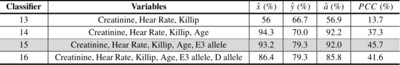
Looking at the best classifiers (classifiers 5 and 15) we then select seven variables: (1) any pre-vious revascularization, (2) systemic arterial hypertension, (3) time elapsed before first medical attention, (4) creatinine, (5) heart rate, (6) Killip classification, and (7) age. To balance the pro-portion between variables identified from each criterion in this set, we have excluded the allele E3 (classifier 15). The first three variables are selected using the disagreement criterion (classifier 5), and the other four variables are selected using the inverse disagreement criterion (classifier 15).
Table 8–ν-SVM with variables selected using the Inverse CZCL Criterion.
Classifier Variables xˆ(%) yˆ(%) aˆ(%) PCC(%)
9 Creatinine, Heart Rate, Age 88.3 68.8 86.6 33.1
10 Creatinine, Heart Rate, Age, HDL cholesterol 51.9 70.4 50.2 13.2
11 Creatinine, Heart Rate, Age, HDL cholesterol, Smoking 57.9 81.5 59.9 35.0 12 Creatinine, Heart Rate, Age, HDL cholesterol, Smoking, Killip 92.3 61.5 89.7 34.1
Note that allele E3 is the last variable included in classifier 15. It provides a 9% increase in sensitivity for classifier 15 with respect to classifier 14, although the specificity and accuracy are reduced by approximately 1% and 0.2%, respectively. On the other hand, this variable ex-cludes one dead individual from the sample used to train classifier 14 because data regarding allele E3 is not available for that particular individual. Given the small number of dead patients, it can be hypothesised that the improvement obtained with the inclusion of allele E3 is not di-rectly attributable to this variable but results from the exclusion of this dead individual. So, we can assume that the most relevant variables for classifier 15 are indeed the first four variables: creatinine, heart rate, Killip and age.
Table 9–ν-SVM with variables selected using the Inverse Disagreement Criterion.
Classifier Variables xˆ(%) yˆ(%) aˆ(%) PCC(%)
13 Creatinine, Hear Rate, Killip 56 66.7 56.9 13.7
14 Creatinine, Hear Rate, Killip, Age 94.3 70.0 92.2 37.3
Next we proceed to train SVM models using several subsets of those seven variables. The re-sults are summarized in Table 10. All subsets include the following three variables: any previous revascularization (first to be selected by the disagreement criterion), creatinine (first to be se-lected by the inverse disagreement criterion) and age. The decision to include age in every subset of variables is justified for two main reasons. First, since age is a variable collected for all indi-viduals its inclusion in a classifier does not exclude any individual from the sample. Second, this variable is less error prone since the level of socioeconomic development in large urban areas prevents the great majority of people from being uncertain about their ages.
Table 10– ν-SVM with variables selected using the Disagreement Criterion and the Inverse Disagree-ment Criterion.
Classifier Variables xˆ(%) yˆ(%) aˆ(%) P CC(%)
17 Creatinine, APR, Age 98.3 87.5 97.5 58.5
18 Creatinine, APR, Age, SAH 98.6 87.5 97.7 58.4
19 Creatinine, APR, Age, Hear Rate 97.6 79.3 96.1 46.7
20 Creatinine, APR, Age, TFM 70.0 75.0 70.4 27.1
21 Creatinine, APR, Age, Killip 63.3 87.1 65.1 37.4
22 Creatinine, APR, Age, SAH, Hear Rate 97.9 79.3 96.4 46.7
23 Creatinine, APR, Age, SAH, TFM 81.1 64.3 79.8 24.9
24 Creatinine, APR, Age, SAH, Killip 64.2 83.9 65.9 33.4
Also observe that including age in the classifier 14 enables us to improve the performance consid-erably with respect to classifier 13: a 35.3% increase in accuracy, a 38.3% increase in specificity and a 3.3% increase in sensitivity. In contrast, the performance of classifier 13 is much worse than that of classifier 9: 29.7% decrease in accuracy, 32.3% decrease in specificity and 2.1% decrease in sensitivity. This finding suggests that the discrimination power of the variable age when used in conjunction with creatinine and heart rate is greater than that of the variable Killip employed with the same two variables.
The best classifiers obtained from the combination of the disagreement and inverse disagree-ment criteria are classifiers 17 and 18. One might argue that systemic arterial hypertension is not relevant since the performance of classifiers 17 and 18 are somewhat similar. To confirm this assumption, a three-variable classifier homologous to the one obtained using the variables creatinine, age and any previous revascularization is evaluated.
In this case, we replace the variable any previous revascularization in classifier 17 by the vari-able systemic arterial hypertension. In contrast to the varivari-ables creatinine and age, which are selected using the inverse disagreement criterion and are non-categorical, the variables any pre-vious revascularization and systemic arterial hypertension are selected using the disagreement criterion and are two-class variables. The performance of the SVM model trained with variables creatinine, systemic arterial hypertension and age is:
ˆ
This result suggests that the variable systemic arterial hypertension is relevant and brings the same kind of information that the variable any previous revascularization does in the presence of the variables creatinine and age. Therefore, both variables (APR and SAH) can be used (although not in the same classifier) to predict the risk of death.
5 CONCLUSION
In this study, we combined the wrapper and filter approaches to select input variables using an incomplete sample. This allowed us to maximize the use of information without resorting to methods for estimating missing data. In the first experiment, we used the order of variables given by the MIFS-U filter to compare the capability ofν-SVM and feed-forward ANN models to predict the risk of death (as high or low) in patients admitted with ACS. In line with previous studies (Berikol et al., 2016; Kumari & Godara, 2011; Xing et al., 2007), the results indicated that theν-SVM model is superior. However, the classifier biases did not diverge in terms of variable selection since both classifiers identified the same optimal subset of input variables: Age, Any Previous Revascularization, and Creatinine.
In the second experiment, we assessed the impact that the MIFS-U filter could have on the vari-able selection and, therefore, on the performance of the models. For this purpose, we developed two new criteria for variable ordering (the disagreement criterion and the inverse disagreement criterion) based on Euclidean distance. These criteria have very low computational cost and are able to capture non-linear relations between input and response variables. Their combined use enabled us to construct classifiers with good performance both in terms of sensitivity and specificity.
Moreover, our Euclidean filters did not only recover the same optimal set of three variables chosen by the MIFS-U filter but also highlighted another set of three equally important vari-ables: creatinine, age and systemic arterial hypertension. So, a possible further advance will be to propose a framework to integrate the classifiers constructed using these two variable groups. For example, this development can enable us to classify the death risk of patients hospitalized with acute coronary syndrome into three classes: high risk, for which both classifiers indicate high risk; moderate risk, for which the classifiers diverge (i.e., one indicates low risk and the other high risk); and low risk, for which both classifiers indicate low risk.
Another possible research stream is to explore causal and explanatory analyses using graphical models such as Bayesian Networks (Pearl, 2009; Schenekenberg et al., 2011) and Chain Event Graphs (Smith & Anderson, 2008; Collazo & Smith, 2015). Finally, in a future study it will also be very interesting to examine the impact of different layers of hidden neurons defined for the ANN algorithm on the results.
ETHICAL STANDARDS
The study protocol conforms to the ethical guidelines of the 1975 Declaration of Helsinki. In Brazil, the Research Ethics Committee of the Faculty of Medicine (Fluminense Federal Uni-versity) and the National Research Ethics Committee approved it. All patients involved in this research signed a consent form. The authors declare that they have no conflict of interest.
ACKNOWLEDGEMENT
The authors would like to thank the reviewers and the editor of the journal for their helpful comments which have greatly improved this paper.
REFERENCES
[1] BALDIP, BRUNAKS, CHAUVINY, ANDERSENCAF & NIELSENH. 2000. Assessing the accuracy of prediction algorithms for classification: an overview.Bioinformatics,16(5): 412–424.
[2] BENNETT KP. 2006. The Interplay of Optimization and Machine Learning Research.Journal of Machine Learning Research,7: 1265–1281. ISSN 15324435. Doi: 10.1051/ps.
URLhttp://portal.acm.org/citation.cfm?id=1248593.
[3] BERIKOLGB, YILDIZO & ¨OZCAN˙IT. 2016. Diagnosis of acute coronary syndrome with a support
vector machine.Journal of Medical Systems,40(4): 1–8.
[4] BISHOPCM. 1995.Neural networks for pattern recognition. Claredon Press, Oxford.
[5] BLUMAL & LANGLEYP. 1997. Selection of relevant features and examples in machine learning. Artificial intelligence,97(1): 245–271.
[6] BOSERBE, GUYONIM & VAPNIKVN. 1992. A training algorithm for optimal margin classifiers. In: Proceedings of the fifth annual workshop on Computational learning theory, pages 144–152. ACM.
[7] BROWNDE & WHITECC. 2012.Operations Research and Artificial Intelligence: The Integration of Problem-Solving Strategies. Springer Netherlands. ISBN 9789400922037.
URLhttps://books.google.com.br/books?id=r\_fnCAAAQBAJ.
[8] CHATFIELDC. 1995. Model uncertainty, data mining and statistical inference.Journal of the Royal Statistical Society. Series A (Statistics in Society),158(3): 419–466.
[10] CHENT, ZHANGC, CHENX & LIL. 2009. An input variable selection method for the artificial neural network of shear stiffness of worsted fabrics.Statistical Analysis and Data Mining,1(5): 287– 295, April.
[11] COLLAZORA & SMITHJQ. 2015. A New Family of Non-Local Priors for Chain Event Graph Model Selection.Bayesian Analysis, Advance Publication, 30 November 2015. Doi: 10.1214/15-BA981. http://projecteuclid.org/euclid.ba/1448852254.
[12] C¸OMAKE & ARSLANA. 2012. A biomedical decision support system using ls-svm classifier with an efficient and new parameter regularization procedure for diagnosis of heart valve diseases.Journal of medical systems,36(2): 549–556.
[13] C¸OMAKE, ARSLANA & T ¨URKOGLU˘ ˙I. 2007. A decision support system based on support vector
machines for diagnosis of the heart valve diseases.Computers in Biology and Medicine,37(1): 21–27. [14] CONCATOJ, PEDUZZIP, HOLFORDTR & FEINSTEINAR. 1995. Importance of events per inde-pendent variable in proportional hazards analysis i. background, goals, and general strategy.Journal of clinical epidemiology,48(12): 1495–1501.
[15] CORTESC & VAPNIKV. 1995. Support-vector networks.Machine learning,20(3): 273–297. [16] DASHM & LIUH. 1997. Feature selection for classification.Intelligent Data Analysis,1: 131–156. [17] REISAF, LHA SALIS, JLR MACRINI, DIASAMC, CHILINQUEMGL, SAUDCGM & LEITERF. 2007. S´ındrome coronariana aguda: morbimortalidade e pr´atica cl´ınica em pacientes do munic´ıpio de Niter´oi (rj).Rev Socerj,20(5): 360–371.
[18] G ´OES ART, STEINER MTA & PENICHE RA. 2015. Classification of power quality considering voltage sags in distribution systems using kdd process.Pesquisa Operacional,35: 329 – 352, 08 2015. [19] GOMES CP. 2000. Artificial intelligence and operations research: challenges and opportunities in
planning and schedulling.The Knowledge Engineering Review,15(1): 1–10.
[20] GONC¸ALVESLB & MACRINIJLR. 2011. R´enyi entropy and cauchy-schwartz mutual information applied to mifs-u variable selection algorithm: a comparative study.Pesquisa Operacional,31(3): 499–519.
[21] GUDADHEM, WANKHADEK & DONGRES. 2010. Decision support system for heart disease based on support vector machine and artificial neural network. In:Computer and Communication Technol-ogy (ICCCT), 2010 International Conference on, pages 741–745. IEEE.
[22] GUYONI & ELISSEEFFA. 2003. An introduction to variable and feature selection.The Journal of Machine Learning Research,3: 1157–1182.
[23] HANNANSA, BHAGILEVD, MANZARR & RAMTEKERJ. 2010. Diagnosis and Medical Prescrip-tion of Heart Disease Using Support Vector Machine and Feedforward BackpropagaPrescrip-tion Technique. International Journal on Computer Science and Engineering,02(06): 2150–2159.
[24] HAYKINSS. 1999.Neural Networks: A Comprehensive Foundation. International edition. Prentice Hall, Upper Saddle River, NJ. ISBN 9780132733502.
[25] HOLSAPPLECW, JOCOBVS & WHINSTONAB. 1994.Operations Research and Artificial Intelli-gence. Intellect Books. Norwood, NJ. ISBN 1567500366.
[27] KHEMPHILAA & BOONJINGV. 2011. Heart disease classification using neural network and feature selection. InSystems Engineering (ICSEng), 2011 21st International Conference on, pages 406–409. IEEE.
[28] KOHLIN & VERMANK. 2011. Arrhythmia classification using svm with selected features. Interna-tional Journal of Engineering, Science and Technology,3(8): 122–131.
[29] KONONENKOI. 2001. Machine learning for medical diagnosis: History, state of the art and per-spective.Artificial Intelligence in Medicine,23(1): 89–109. ISSN 09333657. Doi: 10.1016/S0933-3657(01)00077-X.
[30] KUMARIM & GODARAS. 2011. Comparative study of data mining classification methods in cardio-vascular disease prediction.International Journal of Computer Science and Technology,2: 304–308. [31] KWAKN & CHOIC-H. 2002. Input feature selection for classification problems.Neural Networks,
IEEE Transactions on,13(1): 143–159.
[32] MACKAYDJC. 1992. Bayesian interpolation.Neural computation,4(3): 415–447.
[33] NOCEDALJ & WRIGHTS. 2006.Numerical optimization. Springer Science & Business Media. New York, NY.
[34] PEARLJ. 2009.Causality: models, reasoning, and inference. Cambridge University Press. New York, NY.
[35] PEDUZZIP, CONCATOJ, FEINSTEINAR & HOLFORDTR. 1995. Importance of events per inde-pendent variable in proportional hazards regression analysis ii. accuracy and precision of regression estimates.Journal of clinical epidemiology,48(12): 1503–1510.
[36] PEDUZZIP, CONCATOJ, KEMPERE, HOLFORDTR & FEINSTEINAR. 1996. A simulation study of the number of events per variable in logistic regression analysis.Journal of clinical epidemiology, 49(12): 1373–1379.
[37] PESSOAˆ LAM, LINSMPE, SILVA ACM & FISZMANR. 2015. Integrating soft and hard opera-tional research to improve surgical centre management at a university hospital.European Journal of Operational Research,245(3): 851–861.
[38] PLATTJ. 1999. Fast training of support vector machines using sequential minimal optimization. In: SCHLKOPFB, BURGESC & SMOLAA (Ed.),Advances in Kernel Methods: support vector learning, MIT Press, Cambridge, MA, pp. 185–208.
[39] SAEYSY, INZAI & LARRANAGA˜ P. 2007. A review of feature selection techniques in bioinformat-ics.bioinformatics,23(19): 2507–2517.
[40] SALAPPAA, DOUMPOSM & ZOPOUNIDISC. 2007. Feature selection algorithms in classification problems: An experimental evaluation.Optimisation Methods and Software,22(1): 199–212. [41] SCHENEKENBERGCNM, MALUCELLIA, DIASJS, & CUBASMR. 2011. Redes bayesianas para
eleic¸˜ao da ventilac¸˜ao mecˆanica no p´os-operat´orio de cirurgia card´ıaca.Fisioterapia em Movimento, 24(3): 481–492.
[42] SCHOLKOPFB & SMOLAAJ. 2001.Learning with Kernels: Support Vector Machines, Regulariza-tion, OptimizaRegulariza-tion, and Beyond (Adaptive Computation and Machine Learning). The MIT Press. [43] SCHOLKOPFB, SMOLAAJ, WILLIAMSONRC & BARTLETTPL. 2000. New support vector
[44] SENGURA. 2012. Support vector machine ensembles for intelligent diagnosis of valvular heart dis-ease.Journal of medical systems,36(4): 2649–2655.
[45] SMITHJQ & ANDERSONPE. 2008. Conditional independence and chain event graphs.Artificial Intelligence,172(1): 42–68.
[46] SUYKENSJAK, ALZATEC & PELCKMANSK. 2010. Primal and dual model representations in kernel-based learning.Statistics Surveys,4: 148–183.
[47] TEIXEIRAJ ´UNIORLA, SOUZARM, MENEZESML, CASSIANOKM, PESSANHAJFM & SOUZA
RC. 2015. Artificial neural network and wavelet decomposition in the forecast of global horizontal solar radiation.Pesquisa Operacional,35(1): 73–90.
[48] TURKOGLUI, ARSLAN A & ILKAYE. 2002. An expert system for diagnosis of the heart valve diseases.Expert Systems with Applications,23(3): 229–236.
[49] U ˘GUZH. 2012. A biomedical system based on artificial neural network and principal component analysis for diagnosis of the heart valve diseases.Journal of medical systems,36(1): 61–72. [50] VAPNIKV. 2006.Estimation of dependences based on empirical data. Springer Science & Business
Media. New York, NY.
[51] WOJEWNIK P & KUSZEWSKIT. 2010. From crisp optimization to fuzzy approach and machine learning operations research evolution.Optimum Studia Ekonomiczne,4(48): 81–98.
[52] XINGY, WANGJ, ZHAOZ & GAOY. 2007. Combination data mining methods with new medical data to predicting outcome of coronary heart disease. InConvergence Information Technology, 2007. International Conference on, pages 868–872. IEEE.
[53] YOUNGS & DOWNST. 1998. Carve-a constructive algorithm for real-valued examples.Neural Net-works, IEEE Transactions on,9(6): 1180–1190.
A APPENDIX – EXPLANATORY AND RESPONSE VARIABLES
(See Table 11)
B APPENDIX – ADDITIONAL AND MODIFIED EXPLANATORY VARIABLES
R O DRIG O A B R UNHO S A CO L L A Z O e t a l.
Table 11– Description of the explanatory and response variables.
Class Name Range
Social and Anthropometric
Age Integer number (years)
Explanatory Variables
Body mass index (BMI) Continuous measurement (kg/m2)
Gender Binomial: male or female
Education level
Ordinal classification with five categories: illiterate, primary school (also incomplete), high school (also incomplete), college education (also incomplete), and post-graduation
Smoking Nominal classification with three categories: non-smoker, former smoker, and smoker
Explanatory Variables from Previous myocardial infaction (PMI) Binomial classification: yes or no Previous Cardiovascular History Any previous revascularization (APR) Binomial classification: yes or no
Clinic and Laboratory
Type of acute coronary syndrome (ACS)
Nominal classification with three categories: unstable angina, acute
Explanatory Variables upon
myocardial infarction without ST-segment elevation, and acute
Hospital Admission
myocardial infarction with ST-segment elevation
Heart Rate Integer number
Killip classification (Killip) Ordinal classification with four categories: class I, class II, class III, and class IV
Creatinine Continuous measurement
Diagnostic Explanatory
Systemic arterial hypertension (SAH)
Binomial classification: normal or elevated (systolic arterial pressure
Variables
equal to or above 140 mmHg or diastolic pressure equal to or above 90 mmHg or an individual who takes an anti-hypertensive medication)
Total cholesterol Binomial classification: normal or elevated (cholesterol above 200 mg/dl or an individual who takes a lipid-lowering medication)
Triglyceride Binomial classification: normal or elevated (triblycerides above 150 mg/dl or an individual who takes a lipid-lowering medication)
A C O M P A R A T IVE ST U D Y BET WEEN AN N A N D SVM F O R M ED IC AL PR O G N O S IS
Class Name Range
Diagnostic Explanatory
HDL cholesterol Binomial classification: normal or low (HDL cholesterol below
Variables (cont.)
40 mg/dl or an individual who takes a lipid-lowering medication)
Diabetes mellitus
Binomial classification: negative or positive (fasting glycemia equal to or above 126 mg/dl or prior use of an oral hypoglycemic agent or insulin)
Genetic Explanatory
DD genotype of the Angiotensin
I-Converting-Binomial classification: present or absent
Variables
Enzyme gene polymorphism (DD genotype) DI genotype of the Angiotensin
I-Converting-Binomial classification: present or absent Enzyme gene polymorphism (DI genotype)
II genotype of the Angiotensin
I-Converting-Binomial classification: present or absent Enzyme gene polymorphism (II genotype)
MM genotype of the M235T polymorphism of
Binomial classification: present or absent the Angiotensinogen gene (MM genotype)
MT genotype of the M235T polymorphism of
Binomial classification: present or absent the Angiotensinogen gene (MT genotype)
TT genotype of the M235T polymorphism of
Binomial classification: present or absent the Angiotensinogen gene (TT genotype)
E2E2 genotype of the Apolipoprotein E gene
Binomial classification: present or absent polymorphism (E2E2 genotype)
E2E3 genotype of the Apolipoprotein E gene
Binomial classification: present or absent polymorphism (E2E3 genotype)
E2E4 genotype of the Apolipoprotein E gene
Binomial classification: present or absent polymorphism (E2E4 genotype)
E3E3 genotype of the Apolipoprotein E gene
Binomial classification: present or absent polymorphism (E3E3 genotype)
E3E4 genotype of the Apolipoprotein E gene
Binomial classification: present or absent polymorphism (E3E4 genotype)
Response Variable Death during the hospital stay Binomial classification: yes or no
R
O
DRIG
O
A
B
R
UNHO
S
A
CO
L
L
A
Z
O
e
t
a
l.
Table 12– Description of three additional explanatory variables and re-parametrised genetic variables for the robustness analysis.
Class Name Range
Social and Anthropometric
Physical Activity Binomial classification: sedentary, active
Explanatory Variables (at least 30 minutes, three times a week)
Explanatory Variables from
Family History of Coronary Arterial Disease (FHD) Binomial classification: yes or no Previous Cardiovascular History
Clinic and Laboratory
Time elapsed before first medical attention (TFM) Continuous measurement (hours) Explanatory Variables upon
Hospital Admission
Genetic Explanatory
D allele of the Angiotensin I-Converting-Enzyme gene polymorphism (D allele) Binomial classification: present or absent
Variables
I allele of the Angiotensin I-Converting-Enzyme gene polymorphism (I allele) Binomial classification: present or absent M allele of the M235T polymorphism of the Angiotensinogen gene (M allele) Binomial classification: present or absent T allele of the M235T polymorphism of the Angiotensinogen gene (T allele) Binomial classification: present or absent E2 allele of the Apolipoprotein E gene polymorphism (E2 allele) Binomial classification: present or absent E3 allele of the Apolipoprotein E gene polymorphism (E3 allele) Binomial classification: present or absent E4 allele of the Apolipoprotein E gene polymorphism (E4 allele) Binomial classification: present or absent
a
O
per
ac
ional,
V
ol.
36(
2)
,