C. C. Pellegrini
Department of Thermal and Fluid Sciences DCTEF Federal University of São João del-Rey – UFSJ Praça Frei Orlando 170, Sala 2.15 MD 36307-904 São João del-Rey, MG. Brazil [email protected]G. C. R. Bodstein
Department of Mechanical EngineeringEE/COPPE Federal University of Rio de Janeiro – UFRJ Caixa Postal 68503 21945-970 Rio de Janeiro, RJ. Brazil [email protected]
The Height of Maximum Speed-Up in
the Atmospheric Boundary Layer
Flow Over Low Hills
In this paper, we study the height of the maximum speed-up, l, for atmospheric boundary layer flows over low hills in a neutral atmosphere. A recent analytically-derived expression for l is compared to the results of several other expressions available in the literature. A critical analysis of all these equations is presented and a new constant obtained from field data is proposed for one of them. We find that the new expression describes observational data better than the others. Through an order of magnitude analysis, we also show that the inner layer depth, calculated as the height where inertia and turbulent forces dominate the other terms and balance each other in the x-momentum equation, can also be used to estimate the height of maximum speed-up. Starting from four analytical speed-up profiles available in the literature, we calculate l by searching for the critical points of these speed-up functions, resulting in new equations for l. All these equations are analysed and our results suggest which one of them performs better when compared to field and wind tunnel data.
Keywords: Flow over hills, height of maximum speed-up, inner-layer depth, small scale topographic features, atmospheric boundary layer
Introduction
There is considerable technological interest in estimating the height where the wind speed-up is maximum in the Atmospheric Boundary Layer (ABL) over low hills. Wind energy specialists are often interested in the precise value of this height in order to efficiently site the wind turbines. Since the output power of a wind turbine is proportional to the cube of the wind velocity, a small wind speed-up corresponds to a large power increase. Engineers also need to know the height of the maximum speed-up to calculate the wind loads on structures that are located on the hilltop, such as antennas and transmission towers.1
On the other hand, the correct calculation of the height of the maximum speed-up, usually denoted by l, is also important in itself. The knowledge of l allows for the adequate prediction of the value of the maximum wind speed-up, which can be obtained by substitution of its value in an expression for the vertical profile of the wind velocity, if this expression is available. In addition, numerical schemes can use the value of l as a subdividing height of the flow field in order to separate fine-mesh regions from coarser ones.
Due to the recognition that hills provide a natural way to enhance wind speeds, many mathematical expressions to calculate l
have been proposed in the literature. The most well-known expressions come from the works of Jackson and Hunt (1975) (and Hunt et al., 1988a), Jensen et al. (1984), Claussen (1988) and Beljaars and Taylor (1989), here referred to as JH, JEN, CL and BT, respectively. Walmsley and Taylor (1996) write these expressions as
2 0) 2 / ln( ) /
(l Lh l z = κ , (JH) (1)
2 0 2
2 ) / ( ln ) /
(l Lh l z = κ , (JEN) (2)
constant )
/ ln( ) /
(l Lh l z0 = , (CL) (3)
constant )
/ ( ln ) /
(l Lh n l z0 = . (BT) (4)
Paper accepted July, 2004. Technical Editor: Atila P. Silva Freire.
In Eqns. (1)–(4), Lh is the half-length of the hill, defined following JH as ‘the distance from the hilltop to the upstream point where the elevation is half its maximum’, z0 is the roughness length and κ is the von Karman’s constant. A comparative study of the relative merits of each equation can be found in Walmsley and Taylor (1996). Dividing Eqns. (1) – (4) through by z0 and rewriting the constants in Eqns. (3) and (4) as C1κ2 and Cnκ2, respectively, we obtain
+ +
+ =
h
L l
l ln( ) 2κ2 , (5)
+ +
+ =
h
L l
l ln2( ) 2κ2 , (6)
+ +
+ =
h
L C l
l ln( ) 1κ2 , (7)
+ +
+ =
h n n
L C l
l ln ( ) κ2 , (8)
where l+≡l z0 and Lh+≡Lh z0.
Based on the 210o wind direction case of the Askervein Hill experiment (Taylor and Teunissen, 1985, 1987), Claussen (1988) suggests that C1κ2 = 0.09 in Eq. (7). This implies that C1 = 0.56, for κ = 0.4, a commonly accepted value. After comparison with the results of MSFD, a mixed spectral finite-difference model described in Beljaars et al. (1987), BT suggest two different pairs of values for
n and Cn, depending on the turbulence closure assumed. For the mixing-length model, they suggest n = 1.6 and Cnκ2 = 0.55 in Eq.
(8) and for the E-ε model, n = 1.4 and Cnκ2 = 0.26. This yields Cn =
3.62 and 1.71, respectively.
works published later adopt this assumption and try to verify that the estimate obtained for l from the available expressions do in fact confirm the field data for lmax. Other authors, such as Taylor et al. (1987) and Beljaars and Taylor (1989), acknowledge that there is a difference between l and lmax, but they still compare predictions for l with field data for lmax. Taylor et al. (1987) state that ‘l is probably best considered as a scale height for the inner layer rather than the height at which something specific occurs’. Beljaars and Taylor (1989) point out that ‘since the inner-layer depth, l, has been introduced by means of order of magnitude considerations, its practical definitions is somewhat arbitrary’.
Apart from this issue, much discussion is found in the literature about which one of Eqns. (1)–(4) provides the best estimate for lmax. The following aspects are summarised from Walmsley and Taylor (1996):
• regardless of the expression used to obtain l, authors always consider l=lmax;
• values predicted by JH are too high when compared to field results;
• values predicted by JEN agree well with observed values in the whole range of variation of Lh/z0, but CL gives better agreement at the specific value of Lh/z0 based on which Eq. (3) was calibrated;
• model results suggest a value for n between 1 and 2 in BT; • more observational data is required to resolve definitively
the question of which mathematical expression describes l
best.
In the present study, we obtain an equation for l based on order of magnitude arguments applied to the x-momentum equation for the ABL. The focal point of the work is to evaluate this expression, along with the most common expressions available in the literature, to be able to estimate the height of the maximum speed-up, lmax, through a comparison with the experimental field and wind tunnel data available in the literature.
The analysis is slightly different from the ones generally found in the literature (Taylor et al., 1987). The resulting equation differs from Eq. (6) only by a constant, which needs to be estimated through a comparison with field data. Once the value of this constant is obtained, calculated values of l are compared with available field data and the agreement is shown to be good. Calculated values of l are also compared with those predicted by Eqns. (5)–(8) and are seen to perform better. We also propose a new value for the constant in the CL equation and show that predicted results are at least as good as the ones obtained with the JEN equation. In addition, we confirm that the JEN equation gives better results than the JH equation, suggesting that the latter should be substituted by JEN or CL, corrected with the constant proposed here. Further analysis of the equation for l indicates that the predicted values can also be used to estimate lmax. We also calculate expressions for lmax from the analytical speed-up profiles proposed by Taylor and Lee (1984), Lemelin et al. (1988), Finnigan (1992) and Pellegrini and Bodstein (2002b). The resulting expressions for
lmax are compared to field data, and it can be seen that the results obtained from the profiles of Taylor and Lee (1984) and Lemelin et al. (1988) are rather similar to that of JH.
Order of Magnitude Analysis
Consider an isolated 2D hill in the middle of an otherwise flat terrain of constant roughness length and under a neutrally stratified atmosphere. Following Kaimal and Finnigan (1994), we consider a hill to be a topographical feature with a (horizontal) characteristic length less than 10 km. Based on the height-to-length scale ratios observed in natural hills (1:10), this leads to heights of up to 1 km. Larger topographical features are considered mountains. We also
assume that a hill has a low slope when its average slope does not exceed 10°. For a horizontal length scale of 10 km, the hill height should not exceed 900 m. Lengths smaller than that lead to smaller heights and, therefore, the corresponding hills are said to be low.
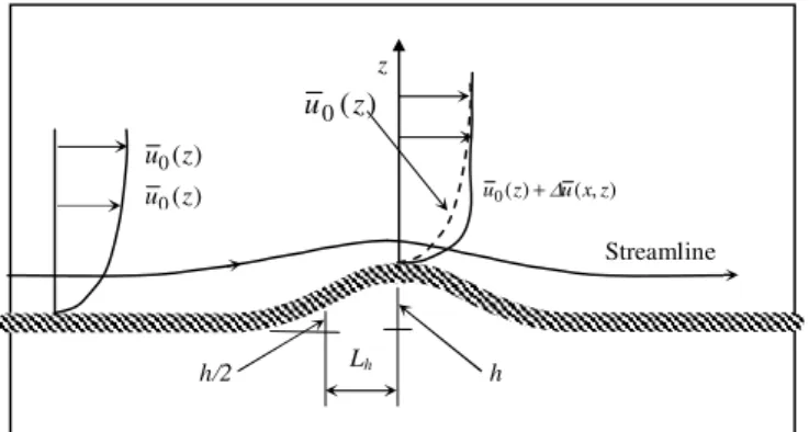
Figure 1 illustrates the main features of a typical low hill. The vertical coordinate z is defined as the height above the local terrain rather than the vertical height above sea level. For the cases of very large roughness elements, z is considered to be the displaced height above the local terrain.
Figure1. Definitions of z, h, Lh, u0 and ∆u.
We assume that the vertical profile of the horizontal mean wind velocity is essentially logarithmic far upwind of the hilltop (HT). This profile is denoted by u0(z), and the location where it is observed is referred to as the reference site (RS). The RS profile suffers the influence of the hill in such a way that it is modified by a speed-up ∆u(x,z), becoming u(x,z) at a given point over the hill. Thus the speed-up is defined as
) , ( ) ( ) ,
(xz u0 z u xz
u ≡ +∆ . (9)
Based on this equation, we define the relative speed-up as
1 ) (
) , ( ) (
) , ( ) , (
0 0
− = ∆ ≡ ∆
z u
z x u z u
z x u z x
S . (10)
The height where ∆u is a maximum is denoted by lmax, whereas the depth of the inner-layer is denoted by l.
In what follows, we develop an order of magnitude analysis of the governing equations to obtain an expression for lmax. We proceed in two steps: first we obtain the expression for the inner layer depth,
l; next, we show that this depth can also be used to estimate the maximum speed-up height, lmax.
Inner-Layer Depth
In order to determine l, we follow Kaimal and Finnigan (1994) and work with the streamlinecoordinate system, which is suitable for distorted flows of this type. The mean x-momentum equation for 2D flows in this system can be obtained from Finnigan (1983). As only the neutral atmosphere case is considered here, the buoyancy term has been neglected. The equation, then, reads
x a
V R
w u L
w u z
w u x u x p x
u
u + − + +
∂ ∂ − ∂ ∂ − ∂ ∂ − = ∂
∂ ' '
2 ' ' ' ' '
1 2 2 2
ρ . (11)
In Eq. (11), x is the direction parallel to the streamlines and u
and u’ are the mean and turbulent velocities in that direction,
Streamline
Lh
h/2 h
) (
0 z
u ) (
0 z
u
) (
0 z
u
) , ( ) (
0z uxz
u +∆
respectively. The direction normal to the streamlines is z, and w’ is the corresponding turbulent velocity. The thermodynamic mean pressure is denoted by p , the mean density by ρ and the
x-component of the mean viscous force by Vx. The quantity R is the local radius of curvature of constant x lines, i.e., the streamlines (Kaimal and Finnigan, 1994). Lais the local radius of curvature of constant z lines. They are related to the mean variables by
)
/( u z
u
R= Ω+∂ ∂ and La=u/(∂u ∂z), where Ω is the mean vorticity component in the y direction of the original Cartesian coordinate system.
Following Taylor et al. (1987), we suppose the existence of a region where the inertia and turbulence terms of Eq. (11) dominate the remaining terms and balance each other, we can write
z w u x u u ∂ ∂ ∼ ∂ ∂ ' '
. (12)
To estimate the order of magnitude of this expression, we assume that x∼Lh and z∼l. We also assume that u∼u0,which means that ∆u<<u. Finally, we assume that u'∼w'∼u*, where
*
u is the friction velocity. With these assumptions, expression (12) becomes l u L l u h 2 * 2 0 ()∼
. (13)
Introducing an unknown function C2(x) of order 1, expression
(13) can be rewritten as u02(l) Lh =C2(x)u*2 l. Rearranging this
equation, we have
) ( ) ( 2 0 2 * 2 l u u x C L l h
= . (14)
Equation (14) is assumed to be valid for the vertical profiles of the incident wind at any x location. If the terrain is flat and the wind profile is logarithmic at RS, we have u0 u*=(1/κ)ln(l z0).
Therefore, Eq. (14) becomes l Lh=C2κ2 ln2(l/z0). Dividing this equation through by z0 and rearranging it, yields
+ + + = h L x C l
l ln2( ) 2( )κ2 . (15)
This equation is identical to that of JEN, except for the constant
C2 that needs to be determined from a direct comparison with observational data.
Height of Maximum Speed-Up
In this section we show that l, predicted by Eq. (15) as the inner-layer depth, can in fact be used to estimate the height of the maximum speed-up. The analysis is different from the one presented in the preceding section for three reasons: the condition of balance between inertia and turbulence is not assumed beforehand; ∆u is introduced in the calculation; and, most importantly, the condition, of maximum ∂∆u ∂z=0 at z=lmax, is explicitly imposed.
Substituting Eq. (9) into Eq. (11) and taking into account that 0
) ( 0 ∂ =
∂u z x and ∆u<<u, we obtain
x a V R w u L w u z w u x u x p x u
u + − + +
∂ ∂ − ∂ ∂ − ∂ ∂ − ∼ ∂ ∆ ∂ ' ' 2 ' ' ' ' '
1 2 2 2
0
ρ .(16)
In order to impose the condition ∂∆u ∂z=0 at z=lmax, we differentiate Eq. (16) with respect to z, and the result is
2 2 2 ' 2 2 0
0 1 ' '
z w u x z u x p z x z u u x u z u ∂ ∂ − ∂ ∂ ∂ − ∂ ∂ ∂ ∂ − ∼ ∂ ∂ ∆ ∂ + ∂ ∆ ∂ ∂ ∂ ρ z V R w u L w u z x a ∂ ∂ + + − ∂ ∂
+ ' ' 2 ' '
2 2
. (17)
To replace the terms in Eq. (17) by their corresponding orders of magnitude, it is necessary to choose an adequate scaling for the pressure term. To first order of approximation, Pellegrini (2001) and Pellegrini and Bodstein (2000, 2002b) show that Euler’s equation, written in streamline coordinates, holds for the ABL flow over hills under neutral atmosphere. Hence,
z p R u ∂ ∂ − = ρ 1 2
. (18)
Equation (18) indicates the scaling −(1/ρ)(∂p/∂z)~u0−2/R.
Substituting this result and the condition ∂∆u ∂z=0 at z=lmax
into Eq. (17), and assuming that x∼Lh, z∼l, u∼u0 and *
' ' w u
u∼ ∼ as before, yields
max max 2 * max 2 * 2 max 2 * max 2 * 2 0 max 0 l V R l u L l u l u L l u RL u L l u u x a h h h + + + − − ∼ ∆ . (19)
Assuming that Lh >> lmax and La >> lmax allows the second and fourth terms on the right-hand side of Eq. (17) to be neglected in comparison to the fourth. In the atmosphere , the viscous term may be neglected by recognizing that it is several orders of magnitude smaller than the other terms, except in the lowest few centimetres above the surface. This fact is generally accepted in the literature, based both on observational data (Stull, 1997) and on scale analysis (Holton, 1992). Equation (19) then simplifies to
R l u l u RL u L l u u h h max 2 * 2 max 2 * 2 0 max
0∆ ∼ − +
(20)
at l=lmax.
The order of magnitude of the terms containing R in Eq. (20) can be evaluated using the definition R=u
(
Ω+∂u ∂z)
, which shows that R∼lmax. Substituting this conclusion into Eq. (20) and recalling again that ∆u<<u yieldsmax 2 * max 2 0 ( )
l u L l u h
∼ . (21)
Equation (21) is formally identical to Eq. (13). Therefore, assuming a logarithmic velocity profile at RS implies that
+ + + = h L x C l
where the function C3(x) can be determined through comparison with observational data, similarly to C2(x).
The preceding analysis shows that Eq. (22) can be used to estimate the height of the maximum speed-up. Since it is identical to Eq. (15), we conclude that thefunction C2(x) can be adjusted so that Eq. (15) also furnishes the height of the maximum speed-up. Therefore, Eqns. (15) and (22) can both be used to estimate the height where inertia and turbulence effects are of the same order of magnitude and the height of maximum speed-up.
Mathematical Expressions for l Obtained from Vertical Velocity Profiles
The availability of a closed-form analytical expression for the speed-up in flows over hills allows for the calculation of the point where its maximum occurs by setting ∂∆u ∂z≡0, at z = l. The maximum itself can also be calculated by substitution of the expression obtained for l into the original speed-up function.
Some expressions for the speed-up function available in the literature can be easily subject to this procedure, whereas others cannot. This analysis applied to Jackson and Hunt’s (1975) solution, for example, does not produce a simple expression for l because their speed-up profile depends on a function that is unknown in the general case. On the other hand, the results proposed by Taylor and Lee (1984), Lemelin et al. (1988) and Finnigan (1992) yield a rather straightforward calculation. In a recent study, Pellegrini and Bodstein (2002a) also obtained an expression for the height of maximum speed-up based on the analytical speed-up function they proposed on a companion paper (Pellegrini and Bodstein, 2002b).
In what follows, the expressions for ∆u(x,z) obtained by Taylor and Lee (1984), Lemelin et al. (1988), Finnigan (1992) and Pellegrini and Bodstein (2002b) are differentiated with respect to z
in order to calculate the value of the height of maximum speed-up.
The Vertical Profile of Taylor and Lee (1984)
Taylor and Lee (1984) propose a relative speed-up vertical profile of the form
h L Az e S z
S( )=∆ max − /
∆ , (24)
where A = 4 for 3-D hills and A = 3 for 2-D hills. In the case of 3-D hills that are elongated in shape, the authors suggest A = 3.5. The definition of ∆S, Eq. (9), implies that
h L Az e S z u z
u( )= 0( )∆ max − /
∆ . (25)
Differentiating this expression with respect to z and setting the result equal to zero at z = l, yields the following expression
] ) / ( ) [(
0=∆Smax ∂u0 ∂z e−Az/Lh+u0 −A Lh e−Az/Lh . Recalling that the velocity profile is logarithmic at the RS, it follows that
− + ∆
= − ln ( / )
0
0 * * /
max Az L A Lh
z z u z u e S h κ
κ , (26)
at z = l. Simplifying and rearranging Eq. (26), we obtain
0 ln 1 z l L A l h
= . (27)
Using the definitions of l+ and Lh+ and after some rearrangement, we can write
+ + + = h L C l
l ln( ) 1*κ2 , (28)
where C1*=1/(Aκ2).
Equation (28) is identical to Eq. (5), derived by JH, or Eq. (7), derived by CL, except for the value of the constant 1/(Aκ2) on the right-hand side. Considering a value of κ =0.4, results in
56 . 1 * 1 =
C , for 3-D hills, C1*=2.08 for 2-D hills and C1*=1.79, for 3-D elongated hills. The value for the 2-D hills is very close to the JH value of 2. In all these cases, however, we conclude that assuming the validity of Taylor and Lee’s (1984) wind profile mathematically leads to the laws of JH or CL for the height of maximum speed-up, from the point of view of an order of magnitude analysis.
The Vertical Profile of Lemelin et al. (1988)
Lemelin et al. (1988) propose the following expression for the relative speed-up
2 2
max 1 3 1
) ( − − + + ∆ = ∆ h p h L z a nL x S z
S , (29)
where a, n and p are constants that depend on the kind of the hill considered. Denoting the term inside the first pair of square brackets by F(x) and using the definition of ∆S, yields
2
max 0( ) ( )1 ) ( − + ∆ = ∆ h L z a x F S z u z
u . (30)
Differentiating Eq. (30) with respect to z, setting it equal to zero at z = l and assuming a logarithmic profile at RS, yields
1 0 1 2 ln 1 − + = h h L l a L a z l
l . (31)
Rearranging Eq. (31) and using the definitions of l+ and Lh+, we finally obtain + + + + − = h L C l l
l 1** 2
2 1 )
ln( κ , (32)
where C1**=1/(2aκ2).
Equation (32) is also similar to Eqns. (5) and (7). According to Lemelin et al. (1988), a = 2 for 3D axisymmetric hills, crests and escarpments, as long as h≤Lh. A value of κ =0.4 produces
56 . 1 * * 1 =
C , which is also relatively close to the value 2 in Eq. (5).
The Vertical Profile of Finnigan (1992)
Finnigan (1992) proposes that
+ + = ∂ ∂ c * 1 α βRi
κ La
where α and β are constants. The parameter La is the curvature radius of the z axis (in the streamline coordinate system), which is given by
x u u
La ∂
∂ = 1 1
. (34)
The remaining parameter in Eq. (33), Ric, is the curvature Richardson number, which is defined as Ric=2u/(ΩR), where Ω is the y-component of the vorticity and R is the radius of curvature of the streamlines.
The analysis of Eq. (33) can be simplified if the dependency of Ric on Ω is eliminated. Using an order of magnitude analysis, Kaimal and Finnigan (1994) show that
R z u
u
* c
Ri ∼ . (35)
Substituting Eq. (9) into Eq. (33), differentiating the result with respect to z, setting ∂∆u/∂z=0 at z = l and supposing a logarithmic profile at RS, yields
+
= * Ric
0 α β
κ La
z z u
, (36)
at z = l. Substituting Eqns. (34) and (35) into Eq. (36) results in
R z u
u x u u
z
* β
α ∼−
∂ ∂
(37)
at z = l.
Substitution of the expression for u obtained from the integration of Eq. (33) into expression (37) produces a recursive loop because Eq. (34) depends on Ric, which, in turn, depends on u again. An alternative to this procedure is to carry out an order of magnitude analysis of Eq. (37) as follows.
Assuming, as before, that x∼Lh, z∼l and u∼u0 in Eq. (37), recalling that the profile is logarithmic at RS, introducing a function
C4(x) to turn the order of magnitude relation into an equality and rearranging the result, yields
2 * 4 0
ln C κ
z l R
Lh =
, (38)
with C4*=(−α β)(C4 κ). Again, C4* must be determined by comparison with observational data.
The Vertical Profile of Pellegrini and Bodstein (2002b)
In recent papers, Pellegrini and Bodstein (2000, 2002b) propose the following new equation for the x-direction mean-wind speed over low hills under a neutral atmosphere:
(
)
(
)
[
h h]
R z
R z R z e
u z x
u h
0
* Ei Ei
) ,
( = −0 −
κ . (39)
In Eq. (39), Ei is the Exponential Integral function, which has well-known properties (Abramowitz and Stegun, 1970), and Rh, called radius length, is a theoretical length used to integrate the equation of motion in the streamwise direction. The parameter Rh is a function of the radius of curvature of the streamlines on the hill’s
surface, i.e., Rh = f(Rh0) = f(Rz=0). One is referred to Pellegrini and Bodstein (2002b) or Pellegrini (2001) for a detailed derivation of Eq. (39). For completeness, a brief derivation is presented in the Appendix. It is worth mentioning that, as Finnigan (1983) points out, the sign of R depends on the sign of Ω. If the center of curvature lies in the direction of increasing z, then R > 0, and vice-versa. For real hills, this means that R < 0 near the HT and R > 0 on the slopes. In the scope of the present solution, the same rule of signs is assumed to hold for Rh.
From Eqns. (9) and (39) and the logarithmic profile at RS, the speed-up function can be written as
(
)
(
)
[
−]
− =∆ −
00 0 * 0
* Ei Ei ln
) ,
( 0
z z k u R z R z e
k u z x
u z Rh h h , (40)
where the friction velocity and the roughness length at RS are denoted by u*0 and z00, respectively. Analysis of Eq. (40), also included in the Appendix, shows that the height of maximum speed-up is
0 *
* 0
ln z
u u R
l h +
= , (41)
where u* is the friction velocity at a specific site and u*0 the friction velocity at RS.
The procedure of setting ∂∆u ∂z≡0, for z=l, finds the critical points of a function, but it does not distinguish a priori between a maximum or a minimum of the function. One way to distinguish them is analyzing the intervals where the function increases and decreases through its first derivative. This analysis is applied to Eq. (41) and can be found in Pellegrini (2001) and in the Appendix. The results show that l is a maximum for Rh<0and u*0<u*, a situation verified in practice at HT, and that l is a minimum for
0 > h
R and u*0>u*, verified in practice on the upwind slope of the HT. Cases with reverse flow are not covered by the theory. In the far more common case, interest is placed on calculating l at the HT, where Rh <0, so that Eq. (41) gives a maximum.
Comparison with Observational Data
We are interested in observational data that allows for the values of C1 in Eq. (7), C2 in Eq. (15) and C4* in Eq. (38) to be calculated. Many field studies provide such data. A list of the most well known sets of observational data can be obtained from the work of Taylor
of comparable logistical scale have been conducted since Askervein, the data still represent a benchmark for such studies’.
Measurements obtained in wind tunnels may also provide useful experimental data for the problem being studied, regardless of their frequent scaling problems. Kaimal and Finnigan (1994) point out that, as a hill is scaled down to fit into a wind tunnel, the surface roughness (grass, heather, stones) usually shrinks too much to satisfy the aerodynamically fully rough condition that ensure flow similarity. This fact, widely recognized in the literature (Britter et al., 1981; Gong and Ibbetson, 1989; Finnigan et al., 1990), reduces the applicability of such measurements. As Athanassiadou and Castro (2001) observe, ‘Laboratory experiments … concentrate on flow that is not always fully rough and, as a result, not directly applicable to the atmosphere.’ The result, reported by Teunissen et al. (1987), for example, falls into this category and, therefore, is not used here.
Although this scaling problem exists, it does not prevents the use of wind tunnel data in our analysis. The usual approach taken to deal with the problem is either to work with an aerodynamically smooth model or to violate the similarity laws and increase the surface roughness length beyond the correct value. Both ways produce measurements that do not represent the near surface properties of real ABL flows exactly. They do only approximately.
This may be a possible explanation for the fact that some authors (Briter et al., 1981; Athanassiadou and Castro, 2001) do not include
l measurements in their otherwise very thorough experiments. Another possibility is to use fully rough models to represent hills covered with rather tall vegetation. Finnigan et al. (1990) and Gong and Ibbetson (1989) report measurements of this kind and their results are included here. These measurements add data to the ‘rough surface end’ of the range, as Figures 2—4 show.
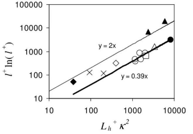
The available field and wind tunnel measurements for l are plotted in Figs. 2 and 3 together with the results of Eqns. (5), (6), (7) and (15) (due to JH, JEN, CL and present work, respectively). The results of Eq. (8) (due to BT) are shown in Fig. 4.
y = 2x y = 2.29x
10 100 1000 10000 100000 1000000
10 100 1000 10000
L
h +κ
2l
+
ln
2
(
l
+
)
Figure 2. Comparison of eqns. (6) and (15) with field and wind tunnel data. Black Mountain: , Askervein Hill: ○, Kettles Hill: ●, BR(max) and BR(min): ▲, BR(1m): ∆, Nyland Hill: ◊, Cooper’s Ridge: □, wind tunnel: X. Eq. (6): ––––, Eq. (15):–––– .
Figure 2 shows that Eq. (6) agrees fairly well with the measured data except for two of the BR (max) and BR (min) results (the dark triangles). Figure 2 also shows the value of C2 = 2.29 that gives the best fit between Eq. (15) and the data using the Least Squares Method, excluding the BR (max) and BR (min) results and passing through the origin. All measurements were made at the HT and, therefore, it is not possible to assess the dependence of C2 on x. With the value obtained with the best fit, Eq. (15) reads,
+ +
+ =
h
L l
l ln2( ) 2.29κ2 . (42)
There has been much discussion in the literature about the value of κ , in particular about the fact that it may not be a constant at all, varying with Re*=u*z0 ν (Frenzen and Voguel, 1995, for example). In this work, we follow Hogstrom (1996) and adopt
4 . 0 =
κ , since this choice affects the value of C2. Apart from this discussion, more field data is necessary before the value of C2, given in Eq. (42), can be stated as definitive.
Comparison between Eq. (5) and the experimental data is shown in Fig. 3. The agreement is only acceptable for the BR(max), BR(min), Black Mountain and Finnigan et al. (1990) wind tunnel data. Mickle et al. (1988), Beljaars and Taylor (1989) and Taylor and Walmsley (1996) has come up with this same conclusion, except for the wind tunnel data, which was not included in their works.
y = 0.39x y = 2x
10 100 1000 10000 100000
10 100 1000 10000
L
h +κ
2l
+
ln
(
l
+
)
Figure 3. Comparison of Eqns. (5) and (7) with observational data. Symbols as in Figure 2. Eq. (5): ––––, Eq. (7): –––– .
According to Taylor et al. (1987), the value of z0 varied between 0.002 and 0.005 m during the BR experiment, and l was 5 m approximately. The two points corresponding to the maximum and minimum values of z0 are represented in Figs. 2—4 as BR(max) and BR(min), respectively. Taylor et al. (1987) point out that the speed-up vertical profile presented a very broad maximum, from the first measurement point up to the height of 8 m. This means that the position of these points in Figs. 2—4 is poorly defined. To illustrate this, a new point was included in the figures, considering z0 equal to 0.0035 m (the average between 0.002 and 0.005 m) and l = 1 m. The value of this new point, represented by BR(1m), is seen to agree very well with the trend of the others in Figs. 2—4. This leads to the conclusion that, given the uncertainties involved in the BR measurements, the agreement between Eq. (5) and the BR data points may be fortuitous. For these reasons, the BR measurements should be considered with caution.
As depicted in Fig. 3, the new value of 0.39 for C1 is obtained by best fitting Eq. (7) to the observational data, excluding BR(max) and BR(min) results and including BR(1m). Agreement is seen to be much better. Thus, Eq. (7) can be rewritten as,
+ +
+ =
h
L l
l ln( ) 0.39κ2 . (43)
The same reasoning was used to exclude the BR(max) and BR(min) data from Fig. 2.
However, more experimental data must be made available before the value of C1=0.39 can be considered the best estimate.
The fact that both Eqns. (42) and (43) describe well the observational data corroborates the conclusion of BT that it is possible to obtain a value for n between 1 and 2 that provides good agreement with the data. In Fig. 4, a comparison is made between Eq. (8), for the two values of n and Cn suggested by BT, and Eq. (42), showing that Eq. (42) describes the observational data better, as a whole, than Eq. (8). As shown in Fig. 4, Eqn (8) describes the
observations slightly better than Eq. (42) in the low Lh+κ2 end (the high l/Lh end of BT’s paper), whereas Eq. (42) describes the remaining experimental data better than Eq. (8). Figure 4 also shows that neither Eq. (8) nor Eq. (42) describes observational data well in the whole range. Nevertheless, it seems reasonable to conclude that Eq. (42) predicts better the experimental data than Eq. (8).
10 100 1000 10000 100000
10 100 1000 10000
L
h
+
κ
2
l
+TW
BT2 BT1
Figure 4. Comparison of Eqns. (8) and (42) with data. Symbols as in Fig. 2. TW: this work, BT1: Eq. (8) with (n,Cn) = (1.4,1.71); BT2: Eq. (8) with (n,Cn) =
(1.6,3.62).
So far, we have observed that Eq. (42) performs better than Eqns. (6) and (8), and slightly better than Eq. (43). This last conclusion can be drawn from the fact that both Eqns. (42) and (43) describe well the field observation, but Eq. (42) is slightly closer to the Black Mountain results (Figs. 2 and 3) than Eq. (43). We also infer that Eq. (5), with its constant equal to 2.0, provides the worst performance of all, and it should definitely be discarded. For this reason, Eqns. (28), (32), (38) and (41) are only compared with Eq. (42) in what follows.
Pellegrini and Bodstein (2002b) compare Eqns. (41) and (42) and show that the former gives consistently better results than the latter. In this analysis, whose results are reproduced here, only the Askervein and Black Mountain data are used, because Eq. (41) requires the knowledge of parameter Rh, which can only be calculated from the vertical velocity profiles measured up to considerable heights.
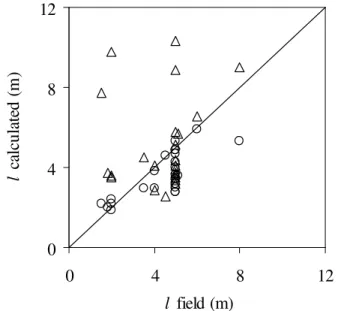
Figure 5 is a comparison between the results of Eqns. (41) and (42) and the Askervein Hill data. In this figure, the distance between the 45o line and the data points represents the difference between calculated and observed values. The analysis of Fig. 5 shows that Eq. (41) indeed describes the Askervein data better than Eq. (42) as a whole. It can be seen that Eq. (42) overestimates the observed data by a considerable amount and presents a higher degree of scattering then Eqn (41). In fact, the average of the differences between calculated and observed values of l is 43.9% for Eq. (42) and – 12.2% for Eq. (41) and the standard deviations are 116.9% for Eq. (42) and 21.9% for Eq. (41). For the only value of l observed over Black Mountain (not represented in Fig. 5), Eq. (42) performs better than Eq. (41). In fact, while Eq. (42) yields l = 15.1 m, underestimating the observed value of 20 m (for all wind velocity
profiles) in 24.5%, Eq. (41) yields l = 41.8 m, which is 109.0% larger than 20 m.
0
4
8
12
0
4
8
12
l
field (m)
l
c
al
cu
la
te
d
(
m
)
Figure 5. Comparison of Eqns. (41) and (42) with the observational data of Askervein. Equation (41): ○; Eq. (42): ∆. Line of lfield = l calculated: ——— .
In spite of the comparisons above, some considerations about the way the height of maximum speed-up is determined from the Askervein and Black Mountain data are worth of note, since they bring up some additional explanations for the scattering in the data.
Experimental values of l are estimated directly from the Askervein and Black Mountain raw data. These estimates are made by computing the difference between the wind velocities at HT and RS for each measurement level and searching for its maximum. However, the limited number of measurement points and the fact that there was often just one point between the supposed maximum and the ground make it very difficult to establish the exact point of maximum ∆u. To overcome this difficulty, a best-fit line for ∆u is drawn and the maximum is estimated directly from it. In all but a few cases, the value estimated for l coincides with the largest experimental value of ∆u. A better estimate could be made in a small number of cases, where two neighbouring points have
u
∆ values very close to each other, suggesting that the maximum is somewhere between them, or cases where the difference in ∆u
values between two neighbouring points is still growing as the ground is approached. As an additional possible source of scattering in the estimation of l, some measurements carried out in 1982 were not taken at the same levels at the RS and HT towers. Therefore, to calculate ∆u we need to interpolate the values of the wind velocity at RS logarithmically at the measuring heights used at HT.
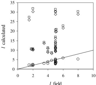
Figure 6 shows a comparison between Eqns. (28), (32) and (41). Eq. (38) was excluded from the comparison because it gives rather poor results. The function C4* is calculated rewriting Eq. (38) as
) ln( ) /
( 2 0
*
4 L R l z
C = h κ h , where R is considered proportional to Rh and the proportionality constant is absorbed into C4*. Using the observational data of Askervein, an average value of C4* = 2054 is determined but with a standard deviation of 468%. This value clearly indicates that C4* is not actually constant.
rather similar to (42) which, in turn, does not perform as well as Eq. (41).
Finally, it is worth pointing out that several authors, such as Kaimal and Finnigan (1994), for example, suggest that a better estimate of l could be obtained from Eq. (5) dividing its results by three. Following this procedure and calculating the differences between the observed and predicted values of l, we get an average difference of 55.8% with standard deviation of 132.9%. If the division factor used is 4.7, which is the same as choosing C1 = 0.39 in Eq. (7), the average difference goes down to 0.6% with standard deviation of 84.8%. This only confirms that Eq. (7) gives the best fit to experimental data, as it has already been shown.
0 5 10 15 20 25 30 35
0 2 4 6 8 10
l
field
l
c
al
cu
la
te
d
Figure 6. Height of maximum speed-up. Comparison between theory and observations. Eq. (28): □, Eq. (32): ◊, Eq. (41): ○. Line of lfield = l
calculated: ——— .
Conclusions
In this paper, we present a study of the height of the maximum speed-up for atmospheric boundary layer flows over low hills under a neutral atmosphere. The flow is assumed to be two-dimensional and the upwind velocity profile is considered to be logarithmic at the reference site. All data used in this work are fully documented in the literature, and they have been acquired during field and wind tunnel studies performed over the hilltop, so that our conclusions are restricted to this point.
Our analysis can be divided in two parts. In the first part, we carry out an order of magnitude analysis on the x-momentum equation to show that the height where inertia and turbulence effects dominate the other terms and balance each other may be used to estimate the height where the maximum speed-up occurs. As a result, we obtain an expression for l that differs from Eq. (6), due to Jensen et al. (1984), only in the value of the constant. We show that this constant can be calibrated so that Eq. (6) gives the height of the maximum speed-up. This procedure yields the new value of C2 = 2.29, which is proposed in Eq. (42). In addition, a new value for the constant in Eq. (7), due to Claussen (1988), is proposed to be C1 = 0.39, resulting in Eq. (43). Still in the first part, we conduct a thorough comparison among four expressions available in the literature, that is, Eq. (5), due to Jackson and Hunt (1975), Eq. (6), due to Jensen et al. (1984), Eq. (7), due to Claussen (1988), Eq. (8), due to Beljaars and Taylor (1989), and the new equations we propose, Eqns. (42) and (43). This study indicates that Eq. (5), which produces the largest errors when compared to the field data,
and Eq. (7), which has been calibrated against one observation only, should be substituted by Eq. (43). Our analysis also shows that Eq. (42) performs better than Eq. (6) because its constant is obtained by direct curve fitting to the experimental data available. Equation (42) also performs better than Eq. (8), considering the entire set of data available.
In the second part of our study, new expressions for l are derived analytically from available speed-up vertical profiles by calculating their critical point through the condition ∂(∆u) ∂z=0, for z=l.
Four profiles are considered: Taylor and Lee (1984), Lemelin et al. (1988), Finnigan (1992) and Pellegrini and Bodstein (2002b). The resulting expressions for l, presented in Eqns. (28), (32), (38) and (41), respectively, allow us to conclude that Eq. (41) performs better than the others and, indeed, better than Eqns. (42) and (43), suggesting that Eq. (41) is the one that provides the best prediction for l.
Further aspects of the study presented here are worth of note. First, we point out that previous good agreement between predictions for lmax and observations for l have hidden the fact that l can be shown mathematically to be a good estimate for lmax, within the validity of the assumptions adopted in the order of magnitude analysis carried out here. This calculation can be used as a new form of obtaining l. An interesting aspect of this calculation is that it makes no use of turbulence closure models and allows for a recalibration of C2(x) if new observational data becomes available. We have shown that Eq. (41) describes the Askervein field data better than the other expressions analysed here. We believe that this is true because Eq. (41) is essentially a dynamic expression. Therefore, it requires that the atmospheric boundary layer equations be fully solved. In other words, it needs z0, u* and Rh to be known in advance. On the other hand, expressions like Eqns. (5) to (8) are easier to use because they are purely geometrical. However, one should consider that:
• Eqns. (5) and (6) also depend on the dynamics of the flow because they include u0(z) implicitly; this is usually where the term ln(l z0) comes from;
• since Eq. (41) comes from a solution of the x-momentum equation for a specific region of the ABL, and not from an order of magnitude analysis, it does not depend on a constant to be calibrated against experimental data; this is a clear advantage, although Eq. (42) does require experimental information to be tuned up for practical use; • the value of l is indeed to be expected to depend on the
dynamics of the flow and the detailed geometry of the hill (expressed through Rh in Eq. (41)) and not only on the ratio
0
z L L+h≡ ,
• the need to calculate z0 and u * is typical of boundary layer solutions based on flux-profile relationships, such as Eq. (41).
which invalidates the assumptions used to obtain Eq. (41). Our analysis also highlights the need to increase the amount of field and wind tunnel data, both at HT, and on the hill slopes, preferably with a higher density of velocity measurements and obtained at the same measuring levels of RS, so that the position of l can be more firmly established along the entire hill surface.
Acknowledgements
The authors wish to thank Dr. Peter A. Taylor, Dr. John L. Walmsley and Dr. Wensong Weng of the Dept. of Earth and Atm. Sciences, York University, Canada, for their kind help. Dr. Taylor has sent us the original tables of wind velocity data from the Askervein hill experiment, whereas Dr. John L. Walmsley has sent the digital data and some reference suggestions and Dr. Wensong Weng has sent the copies of the ‘Guidelines’ works. The authors would like to acknowledge the financial support from National Research Council of Brazil (CNPq), through grants AI 551364/02-5 and APQ 474904/01-6. A shorter version of this work was considered the best scientific paper presented at the Micrometeorology Session of the XII Brazilian Congress of Meteorology, held in Foz do Iguaçu, PR, August 04-09, 2002.
References
Abramowitz, M. and Stegun, I. A., 1970, ‘Handbook of Mathematical Functions with Formulas, Graphs, and Mathematical Tables’, Dover Publications, New York, 9th Edition, 459 p.
Athanassiadou, M. and Castro, I. P., 2001, ‘Neutral flow over a series of rough hills: a laboratory experiment’, Boundary Layer Meteorol., Vol. 101, pp. 1-30.
Beljaars, A. C. M. and Taylor, P. A., 1989, ‘On the inner-layer scale height of boundary layer flow over low hills’, Boundary Layer Meteorol., Vol. 49, pp. 433—438.
Beljaars, A. C. M., Walmsley, J. L. and Taylor, P. A., 1987, ‘A mixed spectral, finite difference model for neutrally stratified boundary layer flow over roughness changes and topography’, Boundary Layer Meteorol., Vol. 38, pp. 273-303.
Bradshaw, P., 1969, ‘An analogy between streamline curvature and buoyancy in turbulent shear flow’, J. Fluid Mech., Vol. 36, pp. 177-191.
Briter, R. E., Hunt, J. C. R. and Richards, K. J., 1981, ‘Airflow over a two-dimensional hill: studies of velocity speed-up, roughness effects and turbulence’, Quart. J. Royal Meteorol. Soc., Vol. 107, pp. 91-110.
Claussen, M., 1988, ‘On the inner layer scale height of boundary layer flow over low hills’, Boundary Layer Meteorology, Vol. 44, pp. 411—413.
Finnigan, J. J., 1992, ‘The logarithmic wind profile in complex terrain’, CSIRO environmental mechanics technical report No. T44, CSIRO, Canberra, Australia, 69 p.
Finnigan, J. J., 1983, ‘A streamline coordinate system for distorted two-dimensional shear flows’, J. Fluid Mech., Vol. 130, pp. 241—258.
Finnigan J. J., Raupach, M. R., Bradley, E. F., Aldis, G. K., 1990, ‘A wind study of turbulent flow over a two-dimensional ridge’, Boundary Layer Meteorol., Vol. 50, pp. 277-317.
Founda, D., Tombrou, M., Lalas, D. P., Asimakopoulos, D. M., 1997, ‘Some measurements of turbulent characteristics over complex terrain’, Boundary Layer Meteorol., Vol. 83, pp. 221-245
Frenzen, P. and Voguel, C. A., 1995, ‘On the magnitude and apparent range of variation of von Karman constant in the atmospheric surface layer’, Boundary-Layer Meteorol.,Vol. 72, pp. 371-392.
Gong, W. and Ibbetson, A., 1989, ‘A wind tunnel study of turbulent flow over model hills’ Boundary Layer Meteorol., Vol. 49, pp. 113-148.
Högström, U., 1996, ‘Review of some basic characteristics of the atmospheric surface layer’, 1996, Boundary Layer Meteorol., Vol. 78, pp. 215-246.
Holton, J. R., 1992, ‘An introduction to dynamic meteorology’, Academic Press, London, 511 p.
Hunt, J. C. R., Leibovich, S. and Richards, K.J., 1988a, ‘The turbulent shear flow over low hills’, Quart. J. Roy. Meteorol. Soc., Vol. 114, pp. 1435-1470.
Hunt, J. C. R., Richards, K.J. and Brighton, P. W. M., 1988b, ‘Stably stratified shear flow over low hills’, Quart. J. Roy. Meteorol. Soc., Vol. 114, pp. 859-886.
Jackson, P. S., and Hunt, J. C. R., 1975, ‘Turbulent wind flow over a low hill’, Quart. J. Roy. Meteorol. Soc., Vol. 106, pp. 929—955.
Jensen, N. O., Petersen, E. L., Troen, I., 1984, ‘Extrapolation of mean wind statistics with special regard to wind energy applications’, Rep. WCP—86, World Meteorol. Organ., Geneva, 85 p.
Kaimal, J. C. and Finnigan, J. J., 1994, ‘Atmospheric boundary layer flows: their structure and measurement’, Oxford Univ. Press, New York, 289 p.
Kaplun, S., 1967, ‘Fluid Mechanics and singular perturbations’, Academic Press, San Diego, 366 p.
Lagerstron, P. A., Casten, R. G., 1972, Basic concepts underlying singular perturbation techniques, SIAM rev., Vol. 14, pp. 63-120.
Lemelin D. R., Surry, D. and Davenport, A. G., 1988, ‘Simple approximations for wind speed-up over hills’, J. Wind Eng. Indust. Aerodyn., Vol. 28, pp. 117-127.
Mellor, G. L., 1972, The large Reynolds number assymptotic theory of turbulent boundary layers, Int. J. Eng. Sci., Vol. 10, pp. 851-873.
Mickle, R. E., Cook, N. J., Hoff, A M., Jensen, N. O., Salmon, J. R., Taylor, P.A., Tetzlaff, G. and Teunissen, H.W., 1988, ‘The Askervein hill project: vertical profiles of wind and turbulence’, Boundary-Layer Meteorol., Vol. 43, pp. 143-169.
Pellegrini, C. C., Bodstein, G. C. R., 2000, ‘A modified logarithmic law for flow over low hills under neutral atmosphere’, in 1st National Congress
of Mechanical Engineering (I CONEM) Natal, RN, Brazil, 7-11 Aug. 2000, in CD ROM.
Pellegrini, C. C., 2001, A modified logarithmic law for the atmospheric boundary layer over vegetated hills under non-neutral atmosphere (in Portuguese), Ph.D dissertation, Federal University of Rio de Janeiro, RJ, Brazil, 142 p.
Pellegrini, C.C. and Bodstein, G.C.R., 2002a, ‘O escoamento em camada limite atmosférica sobre colinas suaves em condições neutras’, anais do XII Congresso Brasileiro Meteorologia (CBMet 2002), Foz do Iguaçu, PR, Brasil, 4 a 9 de agosto, 2002, em CD-ROM.
Pellegrini, C.C. and Bodstein, G.C.R., 2002b, ‘A altura do aumento de velocidade máximo e a altura da região interna no escoamento em camada limite atmosférica sobre colinas’, anais do XII Congresso Brasileiro Meteorologia (CBMet 2002), Foz do Iguaçu, PR, Brasil, 4 a 9 de agosto, 2002, em CD-ROM.
Raupach, M. R. and Finnigan, J. J., 1997, ‘The influence on meteorological variables and surface-atmosphere interactions’, Journal of Hydrology, Vol. 190, pp. 182-213.
Reid, S., 2003, ‘Hilltop wind profiles using SODAR’, Boundary Layer Meteorol., Vol. 108, pp. 315-314.
Roberts, S. M., 1984, ‘A boundary value technique for singular perturbation problems’,J. Math. Analysis Applic., Vol. 87, No. 1, pp. 489-508.
Schilichting, H., 1968, ‘Boundary layer theory’, Ed. McGraw-Hill, New York, 6th edition, 748 p.
Stull, R. B., 1997, ‘An Introduction to boundary layer meteorology’, 6th ed., Dordrecht, Kluwer Ac. Publ., 670 p.
Taylor, P. A. and Lee, R. J.
,
1984, ‘Simple guidelines for estimating wind speed variations due to small scale topographic features’, Climatological bulletin, Vol. 18, No. 2, pp. 3—22.Taylor, P. A., Mason, P. J and Bradley, E. F., 1987, ‘Boundary layer flow over low hills (a review)’, Boundary Layer Meteorology, Vol. 39, pp. 107—132.
Taylor, P. A., and Teunissen, H. W., 1983, Askervein 82: an initial report on the September/October 1982 experiment to study boundary-layer flow over Askervein, South Uist, Scotland, Internal report MSRB-83-8, Atmos. Environ. Serv., Downsview, Ontario, Canada.
Taylor, P. A., and Teunissen, H. W., 1985, The Askervein hill project: report on the September/October 1983 main field experiment, in Internal report MSRB-84-6, Atmos. Environ. Serv., Downsview, Ontario, Canada.
Teunissen, H. W., Shokr, M. E., Bowen, A. J., Wood, C. J., Green, D. W. R., 1987, ‘Askervein hill project: wind-tunnel simulations at three length scales’, Boundary Layer Meteorol., Vol. 40, pp. 1-29.
Townsend, A. A., 1965, ‘Self-preserving flow inside a turbulent boundary layer’, Journal of Fluid Mechanics, Vol. 22, pp. 793—797.
Appendix
In order to obtain Eq. (39), the definition of La is substituted into Eq. (11) to yield
x a
a
V R
w u L
w u z
w u x u x p L
u + − + +
∂ ∂ − ∂ ∂ − ∂ ∂ −
= 1 ' ' ' ' ' 2 ' '
2 2 2
2
ρ , (A1)
An approximate analytical solution to Eq. (A1) can be obtained using the Intermediate Variable Technique, denoted henceforth as IVT (Kaplun, 1967; Lagerstron and Casten, 1972; Mellor, 1972; Roberts, 1984). In this method, the equation under consideration goes through the following steps: nondimensionalization; ‘stretching’ of the z-coordinate through an adequate transformation of variable; variation of the value of a small parameter ε, involved in the stretching process; and collection of the leading order terms of the resulting equation. After the first two of these steps, Eq. (A1) reads
−
− ∂ ∂ + ∂ ∂ − ∂ ∂ −
= ad
a ad
a L
W U W U X U X
P L
U 2 2 2 2
* 2
' ' ' ' 1 '
Z
ε ε
ad x R
ad U V
U W
U ε ε
ε ∂ + ∂ + Ω −
Z
' ' 2
. (A2)
Here, X ≡x L, Z≡z L, U≡u Ug, P≡ p (ρUg2) and
L Ug ad ≡Ω
Ω , where, L is the horizontal length scale of the problem and Ug is the geostrophic wind speed. The turbulence terms are nondimensionalized using the friction velocity, u*. The stretched vertical coordinate Z, of order one, is defined as
L z
Z ε = ε
≡
Z , with ε being the small parameter characteristic of
the IVT. The other small parameters are defined as ε*≡u* Ug and Re
1 ≡ R
ε , with Re≡UgL ν being the Reynolds number. These
parameters are indeed small, since u*<<Ug and Re>>1 in the
ABL. Variables Vxad, Laadand ad
R are the nondimensional counterparts of Vx, La and R respectively.
Variation of the value of ε in Eq. (A2) changes the relative order of magnitude of its terms. For example, putting ε~εR ε*2
implies that ε*2
(
∂U'W'∂Z)
∼εR∂2U ∂Z2, meaning that the turbulence and viscous forces are of the same order in the regiondefined by the transformation, i.e., by ε~z L~εR ε*2 (note that
Z∼1 by definition). This process can be used systematically to
search for every possible value of ε that makes the terms containing
Z change its order. As the value of ε is continuously varied, different
regions are obtained, each characterized by different leading order terms in Eq. (A2).
To submit Eq. (A2) to the last two steps mentioned above, a change in notation is convenient. The advective term on the left-hand side is denoted Ax. On the right-hand side, the pressure term is denoted by Px, the turbulence terms (second and third) by Tx1 and Tx2, the curvature terms (fourth and fifth) by Cx1, and Cx2 and the viscous term (the last) by Vx. Multiplying through by ε2 results in
(
x x x x)
R xx
x P T T C C V
A ε ε ε ε ε ε ε
ε =− − 2 1+ 2− 2 1− 2 +
2 * 2 2
. (A3)
Allowing εto vary in this equation and collecting leading order terms yields the following results:
Advective Region (ε*2<<ε≤1): Ax=−Px;
Turbulent-Advective Region (ε ∼ε*2): Ax=−Px−Tx2+Cx2; Fully Turbulent Region (εR ε*2<<ε<<ε*2): 0=−Tx2+Cx2;
Turbulent-Viscous Region (ε∼εR ε*2): 0=−Tx2+Cx2+Vx; Viscous Region (ε<<εR ε*2): 0=Vx,
where Vx represents the leading order terms of the viscous force and
it is assumed that ε <<R ε*2. This hypothesis is usual in IVT applied to high Reynolds number flows and is based on the fact that as Re increases, εR decreases and ε* increases. Physically, it is supported by comparison with field data.
For the Fully Turbulent Region, a solution can be found substituting the definitions of the nondimensional variables and the small parameters where appropriate and recalling that Z∼1. Hence,
this equation becomes
R w u z
w
u ' '
2 ' '
0 +
∂ ∂ −
= , (A4)
valid for (Ug /u*)2 Re<<z/L<<(u*/Ug)2.
To solve Eq. (A4), its region of validity is supposed to be close enough to the surface so that R(x,z)≈Rh(x,0)≡Rh0(x), where
) ( 0 x
Rh is the radius of curvature of the hill’s surface. It is also assumed that turbulence can be modeled by the Mixing Length Theory in streamline coordinates, with the mixing length given by
z
lm =κ (κ being the von Karman’s constant). With these assumptions, the solution to Eq. (A4) can be written as
z x C
z
u 1( ) ezRh0(x) κ
= ∂ ∂
. (A5)
Equation (A5) can be integrated between z0 and z, assuming that u(x,z0)=0. The result, valid for z≥z0, is
[
] [
]
= ( ) Ei ( ) Ei ( )
) ,
( 0 0 0
1
x R z x R z x C z x
u κ h h . (A6)
The determination of C1(x) requires a boundary condition valid
for the region. Field results show that over flat terrain (u'w') does not vary appreciably with z next to the surface, so that
2 ) , ( '
'w xz u*
u = as z→0. Assuming this behavior to be also valid
for low hills, Eq. (A6) yields C1(x)e2z/Rh0(x) =u*2 as z→0. At
0
z
z= , we can write 1( ) *e 0/ 0( ) x R
z h
u x
C = − . Equation (A6) may, then, be finally rewritten as
= e− Ei( ) Ei( )
) ,
( 0
) ( / * 0
h h
x R z
R z R z u
z x u
h
κ . (A7)
the hypothesis that the Fully Turbulent Region goes down to z = z0. The validity of Eq. (A6) may be extended to hills covered with tall vegetation by a displacement in the origin, as the flat terrain case. Thus, we assume hereafter that z denotes the displaced height.
The height of maximum speed-up can be calculated by setting 0
= ∂ ∆
∂ u z in Eq. (40), which is obtained from Eq. (A7), assuming that this point falls into the Fully Turbulent Region. Noting that
z u z u z
u ∂ =∂ ∂ −∂ ∂
∆
∂ 0 , it follows that
( ) 1 0
e 0
0 *
* 0
* =
−
= ∂ ∆
∂ z−z Rh
u u kz u z
u
, (A8)
Assuming that no reverse flow occurs (u*>0) and noting that 0
0 * >
u and z≥z0'>0, Eq. (A8) is reduced to
( )
0 *
*e 0 u
u zcrit−z Rh = , which yields:
0 *
0 *
ln z
u u R
zcrit h +
= , (A9)
where zcrit >0 is the critical point of ∆u. Equation (A9) implies that u*0>u* if Rh>0 and u*0<u* if Rh<0, which is a well-known experimental fact. To determine if zcrit in Eq. (A9) is a maximum or a minimum, the intervals where ∆u increases and
decreases are analysed. The expression u*e(zcrit−z0)Rh =u*0 is
substituted into Eq. (A8) and the result is
( )
0 * *e 0 increasing
0 u u u
z
u ∂ > ⇒∆ ⇒ z z Rh >
∆
∂ −
(z z0)Rh e(zcrit z0)Rh
e − > −
⇒
( )
0 * *e 0 decreasing
0 u u u
z
u ∂ < ⇒∆ ⇒ z z Rh<
∆
∂ −
(z z0)Rh e(zcrit z0)Rh
e − < −
⇒ . (A10)
For Rh>0, these expressions yield
0 for decreasing
increasing >
∆
⇒
< ⇒∆ >
h crit
crit R
u z
z
u z z
, (A11)
and, therefore, zcrit is the absolute minimum. For Rh<0,
0 for decreasing
increasing <
∆
⇒
> ⇒∆ <
h crit
crit R
u z z
u z
z , (A12)
and, therefore, zcrit is the absolute maximum. In most cases, interest lies in the maximum value, denoted l. Substituting zcrit by l in Eq. (A9) finally yields
0 *
0 *
ln z
u u R
l h +