COMPARISON BETWEEN TWO GENERIC 3D BUILDING RECONSTRUCTION
APPROACHES – POINT CLOUD BASED VS. IMAGE PROCESSING BASED
D. Dahlke a, M. Linkiewicz a
a
DLR, Institute of Optical Sensor Systems, 12489 Berlin, Germany - (dennis.dahlke, magdalena.linkiewicz)@dlr.de
Commission III, WG III/4
KEY WORDS: Building reconstruction, Oblique imagery, Photogrammetric Point Cloud
ABSTRACT:
This paper compares two generic approaches for the reconstruction of buildings. Synthesized and real oblique and vertical aerial imagery is transformed on the one hand into a dense photogrammetric 3D point cloud and on the other hand into photogrammetric 2.5D surface models depicting a scene from different cardinal directions. One approach evaluates the 3D point cloud statistically in order to extract the hull of structures, while the other approach makes use of salient line segments in 2.5D surface models, so that the hull of 3D structures can be recovered. With orders of magnitudes more analyzed 3D points, the point cloud based approach is an order of magnitude more accurate for the synthetic dataset compared to the lower dimensioned, but therefor orders of magnitude faster, image processing based approach. For real world data the difference in accuracy between both approaches is not significant anymore. In both cases the reconstructed polyhedra supply information about their inherent semantic and can be used for subsequent and more differentiated semantic annotations through exploitation of texture information.
1. INTRODUCTION AND MOTIVATION
Photogrammetric companies consider or even decided upgrading their airborne cameras to aerial oblique cameras. These multi view systems increasingly gain importance for building reconstruction because façades have a higher resolution in oblique imagery. Therefor National Mapping and Cadastral Agencies consider changing their production pipelines. Mc Gill (2015) from Ordance Survey Ireland stated that one of the next steps in the production pipeline should be the “Automatic generation of solid objects as an output.” These objects have to provide exact geometrical, topological and semantic descriptions for urban objects like building façades and roof structures.
Another aspect of focusing on the retrieval of solid man-made objects from remote sensing data is given in the outcome of a questionnaire by the European Spatial Data Research Network (EuroSDR): “Vendors seem to focus more on visualisation” like textured CityGML while “Users seem to focus more on semantics” (Gerke, 2015). Both demands rely on simplified objects, since the photogrammetric raw data represented by a 3D pointcloud, a 3D mesh or a surface model lacks the capability to be meaningfully equipped with semantic information. An example for texturing and annotating reconstructed CityGML models with aerial oblique imagery and its classification results can be found in Frommholz et al. (2015).
Nevertheless it is an ongoing research topic to derive complete building structures without a priori knowledge like cadaster information for the building footprints. Within the scope of geometrical and topological reconstruction of buildings from aerial oblique and vertical imagery, this paper presents and compares two methods which fulfill these objectives. On the one hand a dense photogrammetric 3D point cloud and on the other hand photogrammetric 2.5D digital surface models (DSM) depicting a scene from different cardinal directions serve as input for the presented methods. These are two of three
contemporary photogrammetric derivatives from raw oblique imagery, which are investigated. A recent approach which employs a 3D mesh, the third contemporary photogrammetric derivative, as input can be found in Verdie et al. (2015).
The photogrammetric 3D point clouds as well as the mentioned kinds of 2.5D DSMs are direct outputs of current semi-global matching (SGM) algorithms (Hirschmüller, 2011). These 2.5D and 3D datasets require different approaches when being analyzed. Another objective of this paper is to discern advantages and drawbacks of both approaches.
The expertise in company owned 3D camera systems (Brauchle et al., 2015) and partners demanding for automatic 3D extraction workflows right up to 3D CityGML are also motivation to find suitable extraction methods, since there are no out of the box solutions so far.
2. STUDY DATASETS
Both approaches are tested on a real and a synthetic dataset (building), in order to determine influences from real world data. The buildings have either internal step edges, which divides the building more or less into two parts or superstructures and are therefore not easy to reconstruct.
The parameters for the synthesized oblique dataset are comparable to the objectives given in the ISPRS Benchmark for multi-platform photogrammetry (Nex et al., 2015). A tilt angle of 40 degree is chosen for the camera which captures the synthetic scene with 80% overlap along track at a distance of approximately 700 m which yields in a ground sampling distance of 8-12 cm.
A flight campaign over the German islands of Heligoland was conducted using the DLR MACS HALE aerial camera (Brauchle et al., 2015) with slightly more than 80% overlap along track. The two oblique sensors pointing to the left and right have a tilt angle of 36°.
An approach for generating oblique surface models for the extraction of geoinformation is presented in Wieden et al. (2013). Following this approach, the oriented oblique images are pre-processed into (tilted) DSMs. The SGM, which has been initially designed for the creation of 2.5D data from High Resolution Stereo Camera images, is applied to the oblique data as well. Many 2.5D surface models of the same scene from different cardinal directions are the result (see table A1). In combination all pixels from the surface models are transformed into genuine 3D points and merged into a single point cloud (see figure 1).
Since the synthetic building is the only elevated object within the synthetic scene, the surface models are comparable to a normalized surface model (nDSM), which could be generated through dedicated algorithms (Mayer, 2004 and Piltz et al., 2016). That means the relative height of the building is implemented in the absolute height values of the normalized surface models and 3D point cloud. For the real world scene such an nDSM algorithm is already applied. Beside a ground-no ground differentiation there is also a polygon generated, which roughly describes the building outline. Both approaches only take the area inside such a polygon into account.
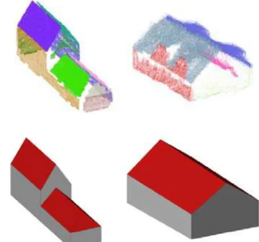
Figure 1. Colored synthetic point cloud (left) and colored point cloud for a building from the Heligoland dataset (right)
3. METHODOLOGY
The presented point cloud based approach is already used for reconstructing roof structures with help of a priori knowledge from cadaster maps (Dahlke et al., 2015). This published approach lacks the capability of reconstructing vertical structures like façades or vertical roof structures. This drawback is overcome by an improvement which is presented in the next section. The image processing approach has similar milestones as the point cloud based. Both start to define planes, which describe facades and the roof of the building. Secondly the topology is recovered by defining edges between the planes. Finally coordinates for the nodes are calculated by intersecting at least three planes.
3.1 Point Cloud Based Approach
The workflow for building reconstruction from 3D point clouds is separated into three steps: identification of cells defining locally coplanar regions, merge of locally coplanar regions into so called building planes, generation of the geometrical model after intersection of building planes.
The idea is to split the 3D point cloud into small spatial areas with a defined size, called cells. For each cell of the grid a linear regression after Pearson (1901) is performed. The regression window of each grid is defined by its 3x3x3 neighborhood. The local regression plane is obtained and defined by points in this neighborhood. The matrix of covariances of a point cloud (1) is a 3x3 matrix and the local regression plane is given in (2).
, , ∈ , , … , (1)
cov ≔
cov , cov , cov , cov , cov , cov , cov , cov , cov ,
(2)
where: cov = matrix of covariance cov=covariance
Three eigenvalues and eigenvectors are calculated for the covariance matrix. The eigenvector corresponding to the smallest eigenvalue is the normal vector n of the regression plane. This plane passes through the center of gravity of the point from the regression window of the considered cell. The square roots of the eigenvalues define the standard deviation in the direction of their corresponding eigenvectors. The relation between the (smallest) standard deviation in the direction of the normal vector of the regression plane and the sum of the other two standard deviations is here defined as a degree of coplanarity:
≔
(3)
where: = degree of coplanarity
= standard deviation in direction of normal vector
2 , 3 = standard deviations in directions of the two other vectors
Cells with degree of coplanarity lower than a certain threshold will be denoted as coplanar cells. Now coplanar cells will be merged into groups defining the so called building planes. A plane cell will be added to a group of plane cells if it has a neighboring cell belonging to this group and if its normal vector is similar to the normal vector of the group of plane cells. The difference of the normal vectors is measured by calculating the angle between the two normal vectors. The normal of the building plane is defined by mean of all normal vectors of a group of plane cells. The result of the merge operation is shown in figure 2. Finally a geometrical model of the whole building is generated. There are two different kinds of intersection points which can be detected: 3-nodes, when three planes build a node or 4-node when four planes build a node. In order to detection of 3-nodes a 3-combination of a set of planes is computed. For each combination is an intersection point calculated. The intersection point is valid and as 3-node indicate, if it lies close to each plane of its triple planes combination. If two valid intersection points lie very close to each other, they are merged into a 4-node. The reconstructed building is shown in figure 2.
Figure 2. Merged groups (top) and reconstructed result (bottom) The International Archives of the Photogrammetry, Remote Sensing and Spatial Information Sciences, Volume XLI-B3, 2016
3.2 Image Processing Based Approach
The idea is to describe the scene with several salient one dimensional edges in 3D space. Filter them in such a way, that it becomes possible to derive 3D planes and subsequently 3D nodes along with a topological description of the 3D object.
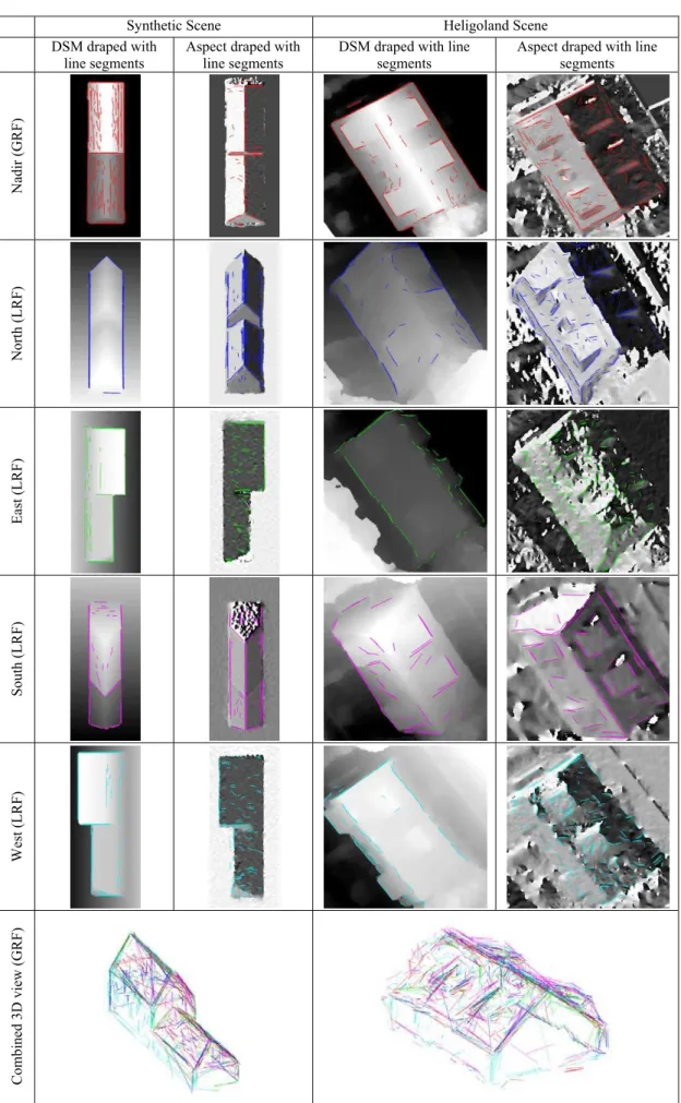
For the detection of salient lines a fast line segment detector (LSD) (Gioi et al. 2010) is used. Since this a gradient based image processing approach some important edges like a roof ridge cannot be detected in surface models as solely input. That is why aspect layers according to Burrough (1998) are derived from the surface models and used as additional inputs for the line segment detection. Both image inputs and the detected line segments for all four cardinal directions as well as the nadir view are gathered in table A1 in the appendix section. The georeferenced 2D coordinates of the line segment’s endpoints are enriched with the height information from the corresponding surface model. Line segments are now described with 3D coordinates for their endpoints in a local reference frame (LRF). The relation between the four LRF is mathematically described in terms of rotation matrices. All line segment coordinates are multiplied with the corresponding transposed rotation matrix to get into a higher level reference frame. A visualization of all detected line segments in 3D-space or global reference frame (GRF) can also be seen in table A1.
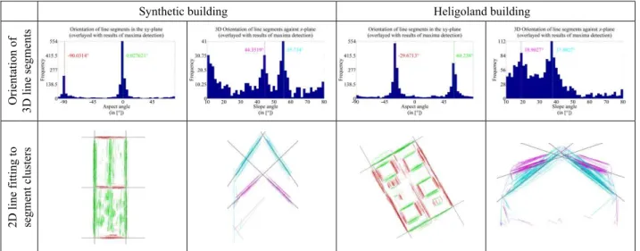
The line segment detection is very sensitive to noise caused by matching inaccuracies in the surface model and artifacts in the aspect layer. To order the chaos, the frequency for attitudes of all segments is analyzed. Attitude in this case means the orientation of a line segment in 3D space that is given on the one hand as horizontal alignment or aspect for façades and on the other hand as vertical alignment or slope for roofs. The ordering of start and endpoints for line segments is of no importance in this case. That means the aspect ranges from -90° to 90°, with -90° and 90° being east-west aligned and 0° being north-south aligned while the slope ranges from 0° to 90°, with 0° being horizontal and 90° being vertical. The histograms for both angles can be found in table 1. They give a first impression of the distribution of predominant angles in the line segments. While the aspect analysis takes all segments into account, the slope analysis is confined to segments which have a predominant aspect angle. Since vertical and horizontal slope
angles are inherently the most prominent features in the slope histogram, the first and last 10° are cut off, so that the range is limited to 10° to 80°. Within the histograms for aspect and slope, a polynomial function of degree 2 is fitted to the peaks. A delta of approximately 90° between two identified aspect angles indicates a good outcome, since most façades are built orthogonally. The maxima are found to be the correct orientation for façade and roof planes. The subsequent process of plane fitting is reduced to two dimensions, since only the position of the planes remains unknown. In case of aspect planes, namely façades it means, that lines are sweeping through the nadir view at the given aspect angles, trying to find significant clusters of line segments. In case of slope planes, namely roofs, the viewing angle is fixed to a horizontal view at the given aspect angles. Again lines are sweeping through the view at given slope angles, in order to find significant clusters of line segments. The fixation of those sweeping lines at clusters marks the position of planes at the previously found orientation angles (see last row of table 1).
In a next step the topology between the planes has to be recovered. For that reason the line segments are used again. All segments are features with a unique ID. While a plane is fitted to a significant cluster of segments, all respective IDs are linked this particular plane. A segment, which two planes have in common, represents a link between planes. A visualization of those linking segments can be found in figure 3. In terms of topology, a building can now be described by planes and edges. With the help of the planes’ geometrical information, namely normal vector and the edges’ topological information, nodes are reconstructed by intersecting three adjacent planes. If more than three planes belong to a node, the point coordinate is recovered by intersecting three planes several times and using the mean of the yielding points of intersections. If two adjacent planes don’t have another plane in common, it may be possible that a 4-node is needed to connect four adjacent planes, which occurs two times on the synthetic building. Therefor the search is extended, in such a way that two adjacent planes are associated to two other adjacent planes if they share common edge relations. The mean coordinate of all possible intersection points is the 4-node. A figure for the reconstructed building basically looks like figure 2 (bottom). More details on the differences of the results can be found in the next section.
dddd
Synthetic building Heligoland building
Orientation of
3D line segments
2D line
fit
ting
to
segment clusters
Table 1. Determination of orientation and position of planes (black lines) through clusters of line segments The International Archives of the Photogrammetry, Remote Sensing and Spatial Information Sciences, Volume XLI-B3, 2016
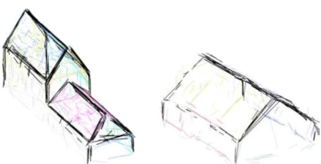
Figure 3. Line segments belonging to different planes are differently colored and line segments belonging to more than one plane are black
4. RESULTS AND COMPARISON
Both algorithms are implemented in a proprietary coding language and tested on the same machine. Concerning quantity figures, it can be stated that the point cloud based approach analyzes millions of 3D points and needs almost 2 minutes to reconstruct a building, while the image processing based approach analyzes hundreds of 3D edges in 5 seconds in order to reconstruct a building.
Since the original model is a synthetic 3D construction, all its nodes are known and used as benchmarks. A comparison between the outcomes of the two approaches for the 16 nodes is given in table 2. The point cloud based approach seems to be statistically much more robust and yields in an average accuracy of 3 cm for 16 nodes. With 25 cm, the average accuracy is an order of magnitude worse for the image processing based approach. The accuracy difference becomes even more obvious when looking at figure 4 (left) which depicts the orthogonal distance between a reconstructed node and the corresponding benchmark plane with color transitions.
Point cloud based approach
Image processing based approach ID Δx Δy Δz Δ3D Δx Δy Δz Δ3D 1 0.01 0.01 0.01 0.02 0.07 0.00 0.06 0.10 2 0.01 0.01 0.02 0.02 0.07 0.00 0.34 0.37 3 0.01 0.02 0.02 0.03 0.08 0.14 0.37 0.41 4 0.00 0.01 0.04 0.04 0.05 0.06 0.04 0.09 5 0.01 0.02 0.04 0.05 0.08 0.14 0.04 0.14 6 0.01 0.01 0.01 0.02 0.01 0.00 0.02 0.02 7 0.00 0.03 0.01 0.03 0.08 0.74 0.02 0.71 8 0.02 0.01 0.04 0.05 0.05 0.00 0.25 0.30 9 0.02 0.02 0.03 0.04 0.04 0.13 0.26 0.32 10 0.01 0.00 0.04 0.04 0.16 0.07 0.04 0.18 11 0.01 0.00 0.01 0.01 0.17 0.01 0.23 0.28 12 0.01 0.00 0.01 0.01 0.17 0.01 0.16 0.25 13 0.02 0.01 0.03 0.04 0.17 0.12 0.22 0.29 14 0.02 0.01 0.04 0.05 0.17 0.12 0.04 0.22 15 0.00 0.01 0.00 0.01 0.05 0.06 0.06 0.10 16 0.00 0.00 0.01 0.01 0.17 0.07 0.17 0.24 min 0.00 0.00 0.00 0.01 0.01 0.00 0.02 0.02 max 0.02 0.03 0.04 0.05 0.17 0.74 0.37 0.71 mean 0.01 0.01 0.02 0.03 0.10 0.10 0.15 0.25 median 0.01 0.01 0.02 0.03 0.08 0.06 0.11 0.25 Table 2. Difference between reconstructed nodes and benchmark values in [cm] for synthetic building
For the Heligoland building reference points have been measured stereoscopically in the oblique and vertical aerial images. The accuracy for these measured points is expected to be not worse than 2 pixel or 14 cm respectively. While the point cloud approach inherently reconstructs the innermost façade edges, the point cloud based approach reconstructs the outermost. That is why the comparison in table 3 contains only two points which are part of both reconstructions, namely the ends of the roof ridge. Both algorithms have comparable mean 3D errors with 30 to 40 cm. A closer look at the errors in z direction reveals that the image processing based approach is way better than point cloud based approach. Compared to the synthetic building the image processing approach remain similarly accurate, while the point cloud based approach is not able to reproduce a very high accuracy. Both algorithms were not able to reconstruct the superstructure on the Heligoland building.
Point cloud based approach
image processing based approach ID Δx Δy Δz Δ3D Δx Δy Δz Δ3D 1 n/a n/a n/a n/a 0.25 0.18 0.03 0.31 2 0.18 0.20 0.04 0.27 0.17 0.18 0.02 0.25 3 n/a n/a n/a n/a 0.26 0.11 0.08 0.30 4 n/a n/a n/a n/a 0.15 0.12 0.12 0.23 5 0.00 0.21 0.41 0.46 0.04 0.08 0.06 0.11 6 n/a n/a n/a n/a 0.31 0.03 0.05 0.32 7 0.12 0.13 0.06 0.19 n/a n/a n/a n/a 8 0.33 0.17 0.22 0.43 n/a n/a n/a n/a 9 0.02 0.21 0.81 0.83 n/a n/a n/a n/a 10 0.17 0.16 0.32 0.40 n/a n/a n/a n/a min 0.00 0.13 0.04 0.19 0.04 0.03 0.02 0.11 max 0.33 0.21 0.81 0.83 0.31 0.18 0.12 0.32 mean 0.15 0.19 0.27 0.42 0.21 0.11 0.06 0.28 median 0.14 0.18 0.31 0.43 0.20 0.12 0.06 0.25 Table 3. Difference between reconstructed nodes and stereoscopic measurements in [cm] for Heligoland building
For a better visual interpretation of the reconstruction, the absolute value of the orthogonal distance between a reconstructed node and the corresponding benchmark plane is used to colorize the planes in figure 4.
Figure 4. Orthogonal distance in [cm] between reconstructed node and benchmark plane for point cloud based approach (top) and image processing based (bottom)
5. CONCLUSIONS AND OUTLOOK
This paper has presented two approaches for the reconstruction of the hull of buildings from oriented oblique and vertical imagery, comparable to recordings from a modern oblique aerial camera system. Regression and image processing methods employing photogrammetric 3D point clouds and vertical 2.5D DSM information respectively were described and compared. Neither building-libraries nor a priori knowledge of the scene is needed. Extracted parts are merged into a fully topologically described 3D building model.
Regarding the average accuracies the quality of the outcome is sufficient to be used for topological linking of CityGML models with a level of detail (LoD) 3, because accuracies are expected to be better than 0.5 meters. The creation of LoD 2 models could be supported without reservations since all absolute accuracies are better than 1 meter. Analysis of the point cloud and 2.5D DSMs have shown that the noise on facades has a standard deviation of 0.4m coming either from the aerotriangulation or the SGM process. Without such a noise, the results, especially for the real world data, are expected to be way better.
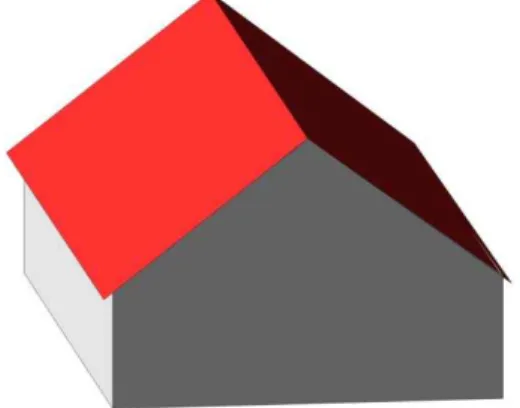
With its advantage in computation speed the image processing based approach is suitable for preliminary results or as support and first guess for the computationally more expensive point cloud based approach. Especially the fusion of both will be focused now. Partly occluded planes which yield in an incomplete respectively distorted point cloud may be correctly reconstructed with salient edges. The presence of super-structures leads to larger errors in the point cloud based approach, since the roof plane is partly fitted to the superstructure too. The image processing based approach detects the slope angle of the roof and superstructure. Just the missing completeness prevents a reconstruction of the superstructure. Another synergy can be found regarding the roof overhang which could be recovered using a combination of both approaches as figure 5 shows with manually mixed nodes for the Heligoland building.
Figure 5. Possible combination of both approaches
REFERENCES
Brauchle, J., Hein, D., Berger, R., 2015 Detailed and highly accurate 3D models of high mountain areas by the MACS – Himalaya aerial camera platform. Int. Archives of Photogrammetry, Remote Sensing and Spatial Information Sciences 40, pp. 1129-1136.
Burrough, P. A., McDonell, R. A., 1998. Principles of
Geographical Information Systems, Oxford University Press,
New York, 190 pp.
Dahlke, D., Linkiewicz, M., Meißner, H., 2015. True 3D Building Reconstruction – Façade, Roof and Overhang Modeling from Oblique and Vertical Aerial Imagery,
International Journal of Image and Data Fusion, vol. 6, no. 4,
pp. 314-329.
Frommholz, D., Linkiewicz, M., Meißner, H., Dahlke, D., Poznanska, A., 2015. Extracting Semantically annotated 3D Building Models with Textures from Oblique Aerial Imagery, in Stilla, U., Heipke, C. (ed.) ISPRS Archives XL-3/W2, pp. 53-58.
Gerke, M., 2015. Preliminary Results from ISPRS/EuroSDR
Benchmark Multi – Platform Photogrammetry, [Online],
Available:
http://www.eurosdr.net/sites/default/files/images/inline/01_gerk e_nex-eurosdr_isprs-southampton2015.pdf [01 Dec 2015].
Gioi, R.G., Jakubowicz, J., Morel, J.M., Randall, G., 2010. LSD: a fast line segment detector with a false detection control, IEEE Trans. Pattern Anal. Mach. Intell. vol. 32 no. 4, pp. 35– 55.
Hirschmüller, H., 2011. Semi-Global Matching – Motivation, Developments and Applications. Invited Paper at the Photogrammetric Week Stuttgart.
Horvat, D., 2012 Ray-casting point-in-polyhedron test.
Proceedings of CESCG 2012: The 16th Central European Seminar on Computer Graphics.
Mayer, S., 2004. Automatisierte Objekterkennung zur Interpretation hochauflösender Bilddaten in der Erdfernerkundung. PhD thesis, Humboldt-Universität zu Berlin.
McGill, A., 2015. LOD2 From Vertical & Oblique Imagery,
[Online], Available: http://www.eurosdr.net/sites/default/files/images/inline/08_mcg
ill-eurosdr_isprs-southampton2015.pdf [01 Dec 2015].
Nex, F., Gerke, M., Remondino, F., Przybilla, H.J., Bäunker,M., Zurhorst, A., 2015. ISPRS Benchmark for Multi-Platform Photogrammetry. ISPRS Annals of the Photogrammetry,
Remote Sensing and Spatial Information Sciences, vol. II-3/W4,
pp. 135-142.
Pearson, K., 1901. On lines and planes of closest fit to systems of points in space. Philosophical Magazine, vol. 2, pp. 559-572.
Piltz, B., Bayer, S., Poznanska, A.M., 2016. Volume based DTM generation from very high resolution photogrammetric DSMs, in ISPRS Archives, in press.
Verdie, Y., Lafarge, F., Alliez, P., 2015. LOD Generation for Urban Scenes. ACM Transactions on Graphics, Association for Computing Machinery, vol. 34, no. 3, pp.1-15.
Wieden, A., Linkiewicz, M., 2013. True- Oblique- Orthomosaik aus Schrägluftbildern zur Extraktion von 3D-Geoinformationen, In: DGPF Tagungsband, vol. 23, pp. 354-362.
APPENDIX A
Synthetic Scene Heligoland Scene
DSM draped with line segments
Aspect draped with line segments
DSM draped with line segments
Aspect draped with line segments
Nadir (GRF)
North (LRF)
East (
L
RF
)
South (LRF)
Wes
t (
L
RF
)
Combin
ed 3D v
iew (GRF
)
Table A1. Line Segment Detection on all 2D input datasets with combined 3D view for all line segments