A FINITE VOLUME METHOD FOR SOLVING GENERALIZED NAVIER-STOKES EQUATIONS

A FINITE VOLUME METHOD FOR

SOLVING GENERALIZED

NAVIER-STOKES EQUATIONS

Stelian Ion† _{Anca Veronica Ion}‡

Abstract

In this paper we set up a numerical algorithm for computing the flow of a class of pseudo-plastic fluids. The method uses the finite vol-ume technique for space discretization and a semi-implicit two steps backward differentiation formula for time integration. As primitive variables the algorithm uses the velocity field and the pressure field. In this scheme quadrilateral structured primal-dual meshes are used. The velocity and the pressure fields are discretized on the primal mesh and the dual mesh respectively. A certain advantage of the method is that the velocity and pressure can be computed without any artificial boundary conditions and initial data for the pressure. Based on the numerical algorithm we have written a numerical code. We have also performed a series of numerical simulations.

MSC_{: 35Q30, 65M08, 76A99, 76D05, 76M12.}

keywords: generalized Navier-Stokes equations, pseudo-plastic fluids, finite volume methods, admissible primal-dual mesh, discrete derivatives operators, discrete Hodge formula.

∗_{Accepted for publication on December 30, 2010.}

†_{ro_diff@yahoo.com ”Gheorghe Mihoc-Caius Iacob” Institute of Statistical}

Mathemat-ics and Applied MathematMathemat-ics, Bucharest, Romania; Paper written with financial support of ANCS Grant 2-CEX06-11-12/2006.

‡_{”Gheorghe Mihoc-Caius Iacob” Institute of Statistical Mathematics and Applied}

Math-ematics, Bucharest, Romania.

145

1

Introduction

In this paper we are interested in the numerical approximation of a class of pseudo-plastic fluid flow. The motion of the fluid is described by the generalized incompressible Navier-Stokes equations

( _∂u

∂t +u· ∇u =−∇p+∇ ·σ(u) +f,

∇ ·u _{= 0,}

(1)

whereu _{is the velocity vector field, p is the hydrodynamic pressure field, σ}

the extra stress tensor field andf _{is the body force. The extra stress tensor}

σ(u_{)obeys a constitutive equation of the type}

σab(u) = 2ν(|∂fu|)∂ufab (2)

where∂uf is the strain rate tensor given by

f

∂uab=

1

2(∂aub+∂bua),

∂a standing for the partial derivative with respect to the space coordinate

xa, and for any square matrixe,|e|being defined as

|e_|=



X

i,j

e2_ij

 

1/2

.

Concerning the viscosity functionν(s),we assume that it is a continuous differentiable, decreasing function, with bounded range

0< ν∞≤ν(s)≤ν0<∞,∀s >0,

(ν(s1)−ν(s2)) (s1−s2)<0,∀s1, s2>0, (3)

and it satisfies the constraint

ν(s) +sν˙(s)> c >0. (4)

The model of the Newtonian fluid corresponds to ν=constant.

We consider the case when the flow takes place inside a fixed and bounded domain Ω ⊂R2 _{and we assume that the fluid adheres to its boundary ∂Ω,}

u₌u_{D(x), x∈∂Ω, t >0. (5)}

To the equations (1) we append the initial condition for the velocity

u_{(x,0) =}u_{0(x), x∈Ω. (6)}

The initial boundary value problem (IBV), which we intend to solve nu-merically, consists in finding the velocity field u_{(x, t) and the pressure field}

p(x, t) that satisfy the partial differential equations (1), boundary condition (5) and the initial condition (6).

A constitutive function as (2) is used , for example, to describe the be-havior of polymeric fluids, [5], [8], [11], and the flow of the blood through the vessels, [19], [9], [6], [18].

In writing down a numerical algorithm for the non-stationary incom-pressible generalized Navier-Stokes equations three main difficulties occur, namely: (i) the velocity field and the pressure field are coupled by the in-compressibility constraint [12], (ii) the presence of the nonlinear convection term and (iii) the nonlinear dependence of the viscosity on the share rate.

The first two problems are common to the Navier-Stokes equations and in the last fifty years several methods were developed to overcome them: the projection method, [12], [13], [7],[14], [3], and gauge method, [20]- to mention the most significant methods for our case.

When one deals with a non-Newtonian fluid, the nonlinearity of the vis-cosity rises a new problem in obtaining a discrete form for the generalized Navier-Stokes equations. The new issue is the development of an appropriate discrete form of the action of the stress tensor on the boundary of the volume-control. A similar dificulty is raised by the discretization of the p-laplacean, see [2] for that.

2

The Existence of the Weak Solution

To define the weak solution we need the following functional frame, [16], [17]. ByLp(Ω)andWm,p(Ω),m= 0,1,· · ·,we denote the usual Lebesgue and Sobolev spaces, respectively. The scalar product in L2 is indicated by(·,·). Foru_, v _{vector functions defined onΩ we put}

(u_,v_{) =}

Z

Ω

uavadx,

(∇u_,∇v_{) =} X

a,b=1

Z

Ω

∂aub∂avbdx.

We denote by|| · ||the norm in L2 associate to (·,·). The norm inWm,p is denoted by|| · ||m,p. Consider the space

V ={ψ∈C₀∞(Ω),divψ= 0}.

We define H_{(Ω)the completion of V in the space} L2_{(Ω). We denote by} H1_{(Ω)the completion ofV in the space} W1,2_.

ForT ∈(0,∞]we set QT = Ω×[0, T) and define

VT ={φ∈C0∞(QT); divφ(x, t) = 0 in QT}.

The weak solution of IBV is defined as follow.

Definition 1. Let f _∈L2_{(Ω). Let}u_0(x)∈L2_{(Ω) anduD be such that}

  

divu_{0 = 0,}

u_D·n_{= 0, x∈∂Ω,} u_{0 =}u_{D, x∈∂Ω,}

(7)

and there existsv_∈W1,2_(Ω)∩L4_{(Ω) a vector function that satisfies}

divv_{= 0,}

v₌u_{D, x∈∂Ω.} (8)

Thenu _{is a weak solution of IBV (1,5,6) if}

andu _verifies

−

∞ Z

0

u_,∂φ

∂t

dt−

∞ Z

0

(u_⊗u_{,∇φ) dt+}

∞ Z

0

σ(u_),∂φf_dt=

=

∞ Z

0

(f_{, φ) dt+ (u0, φ)}

(10)

for any test functionφ∈ VT.

Concerning the existence of the weak solution of the IBV we proved the following result, [15]:

Theorem 1. If the constitutive function ν(·) satisfies the relations (3) and (4)then there exists a weak solution of the IBV (1), (5)and (6).

3

Semi-discrete Finite Volume Method

The finite volume method (FVM) is a method for approximating the solution of a partial differential equation (PDE). It basically consists in partitioning the domainΩ, on which the PDE is formulated, into small polygonal domains ωi (control volumes) on which the unknown is approximated by constant

values, [10].

We consider a class of finite-volume schemes that includes two types of meshes: the primal mesh, T ={ωI,rI} and the dual mesh, Te = {ωeJ,erJ}. The space discrete form of the GNS equations are obtained from the integral form of the balance of momentum equation and mass balance equation on the primal mesh and the dual mesh respectively.

For any ωi of the primal mesh T the integral form of the balance of

momentum equation reads as,

∂t Z

ωi

u₍x_{, t)dx+}

Z

∂ωi

uu_·n_ds+

Z

ωi

∇pdx=

Z

∂ωi

σ·n_{ds, (11)}

and for anyω_eαof the dual meshTethe integral form of mass balance equation

is given by _Z

∂ωeα

The velocity field u₍x_{, t) and the pressure field p(}x_{, t) are approximated}

by the piecewise constant functions on the primal mesh and the dual mesh respectively,

u₍x_{, t)≈}u_i(t),∀x_{∈ωi, p(}x_{, t)≈pα(t),∀}x_∈ωeα.

By using certain approximation schemes of the integrals as functions of the discrete variables{ui(t)}i∈I,{pα(t)}α∈J one can define:

Fi(u)≈R_∂ωiuu·nds, Si(u)≈R_∂ωiσ·nds,

Grad_i(p)≈R

ωi∇pdx, ,Divα(u)≈

R

∂eωαu·nds.

(13)

The semi-discrete form of GNS equations, continuous with respect to time variable and discrete with respect to space variable, can be written as:

mi

du_i

dt +Fi({u}) +Gradi({p})− Si({u}) = 0, i∈ I Divα({u}) = 0, α∈ J

(14)

wheremi stands for the volume of theωi.

Now the problem is to find the functions{u_{i(t)}i∈I,{pα(t)}α∈J that}

sat-isfy the differential algebraic system of equations (DAE) (14) and the initial condition

u_i(t)|

t=t0 =u

0

i, ∀i∈ I. (15)

In solving the Cauchy problem (14) and (15), an essential step is to define a primal-dual mesh T,Te that allows one to calculate the velocity field independent of the pressure field.

In the next subsections we define a pair of quadrilateral admissible primal-dual (QAPD) meshes T,Te, and we define the discrete gradient of the scalar functions and the discrete divergence of the vector functions such that the discrete space of the vector fields admits an orthogonal decomposition into two subspaces: one of discrete divergences free vectors fields, and other consisting of vectors that are the discrete gradient of some scalar fields.

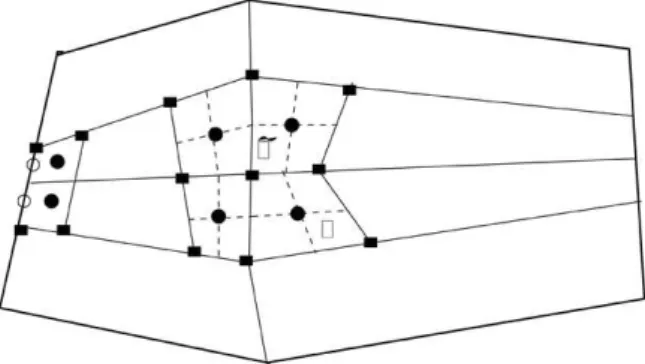
3.1 Quadrilateral primal-dual meshes

Let Ω be a polygonal domain in R2_{. Let T = {ωI,}r_{I} be a quadrilateral}

(1)ωi is a quadrilateral,∪i∈Iωi = Ω,

(2)∀i6=j∈I and ωi∩ωj 6= Φ,eitherH1(ωi∩ωj) = 0, or

σij :=ωi∩ωj is a common (n−1)−face of ωi andωj,

(3)r_{i∈ωi,if ωi= [ABCD], then}r_{i = [MABMDC]∩[MADMBC],}

(4) for any vertex P∈Ω there exists only four quadrilateralω with the common vertex P,

whereH1 is the one-dimensional Hausdorff measure, and MAB denotes the

midpoint of the line segment [AB].

LetTe ={ω_eJ,erJ}be another mesh defined as follows:

(1)∀α∈ J, _er_{α is a vertex of T,}

(2)_er_{α∈eωα,∀α∈ J,}

(3)∀_er_{α∈Ω,the poligon ωeα has the vertexes :}

the centers of the quadrilaterals with the common vertex_er_α

and the midpoints of the sides emerging fromer_α,

where by "center" of the quadrilateral we understand the intersection of the two segments determined by the midpoints of two opposed sides.

Figure 1: Quadrilateral mesh.

We call (T,Te) - a pair of QAPD meshes.

We denote by H_Te(Ω) the space of piecewise constant scalar functions that are constant on each volumeω_eα ∈ωeJ, byHT(Ω)the space of piecewise constant vectorial functions that are constant on each volume ωi ∈ ωI and by H_⊗H_e

T(Ω)the space of piecewise constant tensorial functions of order two that are constant on each volumeω_ea∈eωJ.

For any quantityψthat is piecewise constant onω_eJ we denote byψαthe

constant value ofψ onω_ea, analogouslyψi stands for the constant value of a

We define the discrete derivative operators: Div_(T,Te) :H_T(Ω)→He

T(Ω), by

Divα(u) := Z

∂ωeα

u_·n_ds=X

i

ua_i

Z

∂eωα∩ωi

nads, (16)

∂_(T,Te):H_T(Ω)→H_⊗H_e

T(Ω)by

∂bua|_α =:

1 m(ω_eα)

Z

∂ωeα

ubnads=

1 m(ω_ea)

X

i

ub_i

Z

∂ωeα∩ωi

nads, (17)

Grad

(T,Te):HTe(Ω)→HT(Ω)by

Grad_i(φ)

Z

∂ωi

φn_ds=X

α

φα Z

∂ωi∩ωeα

n_{ds, (18)}

rot

(T,Te):HTe(Ω)−→HT(Ω)by

rot_{i(φ) :=} 1

m(ωi) Z

∂ωi

φdr₌ 1

m(ωi) X

α

φα Z

∂ωi∩ωeα

dr_{. (19)}

On the space H_{T(Ω)we define the scalar product hh·,·ii by}

hhu_,v_ii=X

i∈I

u_i·v_{i, (20)}

and on the space H_Te(Ω)we define the scalar producth·,·i by

hφ, ψi= X

α∈J

φαψα. (21)

In the next lemma we prove certain properties of the discrete derivative operators.

(a1) Discrete Stokes formula. For any u _∈ H_{T(Ω) and any φ ∈ He}

T(Ω), a discrete integration by parts formula holds, that is

D

Div_(T,Te)(u_{), φ}E₊DDu_,Grad

(T,Te)(φ)

EE

= 0. (22)

(a2) For anyψ∈H_Te(Ω), ψ|_∂Ω= 0 one has

Div_(T,Te)rot

(T,Te)ψ= 0. (23)

Proof. To prove (a1) we use the fact that for any domain ω

Z

∂ω

n_{ds= 0}

and the definitions of the two operators. To prove (a2), we note firstly that

Divα(rot_(T,Te)ψ) =

X

i

rot_i(ψ)·

Z

∂ωeα∩ωi

n_ds=

=X

i

1 m(ωi)

X

β

ψβ Z

e ωβ∩∂ωi

dr_·

Z

∂ωeα∩ωi

n_ds.

Then, let ωiα

a, a= 1,4 be the primal volumes with the common vertex Pα and numbered such thatωiα

a andωiαa+1 have a common side. For eachi

α a let

P

αiαa b

,b= 1,4be the vertexes of the quadrilateralωiα

a anticlockwise numbered andP

αiαa

1

=Pα. We have

1 m(ωia)

X

b

ψ

αiαa b

Z

e ω

αiαa b

∩∂ωiαa dr_·

Z

∂eωα∩ω_ia

n_ds=ψ

αiαa

2

−ψ

αiαa

4 .

Finally, by summing up fora= 1,4,we have

Divα(rot_(T,Te)ψ) =

X

a

(ψ

αiαa

2

−ψ

αiαa

4

) = 0,

for any α such that Pα ∈ Ω. If for some α, Pα ∈∂Ω, we use the fact that

Now we prove an orthogonal decomposition of the space H_{T(Ω) that}

resembles the one for the non-discrete case. Let {Ψα}α∈J,Ψα ∈HTe(Ω)be

a basis of the spaceH_Te(Ω)given by

Ψα(x) =

1, if x∈w_eα_,

0, if , x /∈w_eα. (24) Define the discrete vector fieldUα∈H_T(Ω)by

Uα=rot_(Ψα_{). (25)}

LetW_{T(Ω)be the linear closure of the set{U}α_{;α∈Int(J)}in the space} H_{T(Ω)and let} G_{T(Ω)be the subspace orthogonal to it, so that}

H_{T(Ω) =}W_T(Ω)⊕G_{T(Ω). (26)}

We state and prove the following proposition.

Proposition 1. G_T(Ω)consists of elements Grad

(T,Te) with φ∈HTe(Ω). Proof. Letu_∈G_{T(Ω), i.e.}

hhu_,Uα_{ii= 0,∀α∈Int(J). (27)}

We construct a function φ∈H_Te(Ω)such that

Grad_{i(φ) =}u_{i, ∀i∈ I.}

For a given ωi we denote by Pαi

b, b = 1,4 its vertexes counterclockwise numbered. The gradient of a scalar fieldφ can be written as

Grad_{i(φ) =}−→_{τ 1,3(φ}

αi

3 −φα

i

1) +

− →_τ

2,4(φαi

4 −φα

i

2),

where−→τ 1,3 is a vector orthogonal to

−−−−→

P_αi

2Pαi4 oriented from Pαi1 to Pαi3 and

|−→τ 1,3| =

−−−−→P_αi

2Pαi4

/2 and −→τ2,4 is a vector orthogonal to

−−−−→

P_αi

1Pαi3 oriented fromP_αi

2 to Pαi4 and |−

→_τ

2,4|=

−−−−→P_αi

1Pαi3

/2. Hence, we have

u_i·−−−−→_P

αi

2Pαi4

m(ωi)

=φ_αi

4−φα

i

2,

u_i·−−−−→_P

αi

1Pαi3

m(ωi)

=φ_αi

3−φαi1.

The point is that if u _{satisfies the ortogonalty conditions (27) then one can}

solve the equations (28) inductively, i.e. starting from two adjacent values and following some path of continuation. For a general discrete field u _the

different paths lead to different values!

Corollary 1 (Discrete Hodge formula). Let (T,Te) be a pair of QAPD meshes. Then for any w _∈ H_{T(Ω) there exists an element} u _∈ H_T(Ω)

and a scalar function φ∈H_Te(Ω) such that

w₌u₊Grad_{(φ) with Div}

(T,Te)(u) = 0. (29)

Proof. We search for a divergence free vectoru _{of the form}

u₌ X

a∈J αaUa.

By inserting this form into (29), one obtains a linear algebraic system of equation for the determination of the unknowns {αa}a∈J,

DD

w_,UbEE₌ X

a∈J αa

DD

Ua,UbEE.

The matrix of the system is the Gram matrix of a linear independent family, hence there exists an unique solution u_.

Sincehhw₋u_,Ua_{ii= 0for any function in the basis, it follows that}w₋u

is orthogonal to G⊥_{, thus} w₋u_∈ G_{. Hence there existsφ∈ He}

T(Ω) such that

w₋u₌Grad_(φ).

3.2 Discrete convective flux and discrete stress flux

To cope with the boundary value problems one defines a partition{∂kω}k∈K of the boundary ∂Ωmesh induced by the primal mesh i.e

∂kω=∂Ω∪∂ωik, ∂Ω =∪k∈K∂kω.

On each ∂kω the boundary data uD are approximated by constant values

u_{D k.}

In the case of a hyperbolic equation, the numerical convective flux must satisfy, besides the accuracy of the approximation requirements, a number of conditions in order that the implied solution be physically relevant. In the case of Navier-Stokes equation at high Reynolds number, the way in which NCF is evaluated is also very important. We propose to define the NCF as follow. Consider the tensorial productu_⊕u _{constant on the dual mesh and,}

for any control volume ωi that does not lie on the boundary F, set for the

NCF:

F_ia=X

α

(uaub)α Z

e ωα∩∂ωi

nbds. (30)

The tensorial productu_⊕u _{is approximated by}

(uaub)α=

1 m(ω_eα)

Z

e ωα

uadx 1 m(ω_eα)

Z

e ωα

ubdx. (31)

The numerical stress flux is set up by considering that the gradient of the velocity is piecewise constant on the dual mesh. This fact implies that the stress tensor is also piecewise constant on the dual mesh. So we can write for the numerical stress flux

Si(u) = X

α

σα(u)· Z

∂ωi∩ωeα

n_{ds. (32)}

The values of σα(u) are evaluated as

σα(u) = 2ν(|Dα(u)|)Dα(u), (33)

where the discrete strain rate tensorD_{α is given by}

Dab(u)|_α=

1 2 (∂au

b_+∂ bua)

α. (34)

Dirichlet Boundary conditions. The boundary conditions for the veloc-ity are taken into account through the numerical convective flux and numer-ical stress flux. If for someαthe dual volume_eωαintersects the boundary∂Ω

the gradient of the velocity is given by:

∂aub

α=

1 m(ω_eα)

Z

∂ωeα

= 1 m(_eωα)

  

Z

∂exteωα

ub_Dnads+ X

i

ub_i

Z

∂intωeα∩ωi nads

 

. (35)

For a primal volume ωi adjacent to the boundary ∂Ω the NCF (30) is

given by

F_ia=ua_Dub_D

Z

∂Ω∩∂ωi

nbds+ X

α

(uaub)α Z

Ω∩∂ωi

unbds. (36)

4

Fully-Discrete Finite Volume Method

We set up a time integration scheme of the Cauchy problem (14) and (15) that determines the velocity field independently on the pressure field. The pressure field results from the discrete balance momentum equation (14-1). The scheme resembles the Galerkin method and it makes use of the orthogo-nal decomposition (26) of the spaceH_{T(Ω)and of the set of divergence free}

vectorial fields {Uα_} α∈J0.

We write the unknown velocity fieldu_{(t)as linear combination of{U}α_}α∈J0

u₌X

α

ξα(t)Uα (37)

where the coefficientsξα(t)are required to satisfy the ordinary differential

equations

X

α

dξα

dt

DD

mUα,UβEE+DDF(ξ),UβEE−DDS(ξ),UβEE= 0,∀β ∈ J0, (38)

with the initial conditions

X

α

ξα(0) DD

Uα,UβEE=DDu0_,UβEE_{, ∀β ∈ J}0_{. (39)}

If the functionsξαsatisfy (38) and (39) thenmd

u

dt+F({u})−S({u})belongs to the space G_{T(Ω) which implies that there exists a scalar field p(t) such}

that

−Grad

(T,Te)p=m

du

Concerning the initial conditions (15), we note that for t = 0 the solution (37) equals notu0 but its projection on the space W_T(Ω).

Now we develop a time integration scheme for the equation (38) derived from two steps implicit backward differentiation formulae (BDF).

Let {tn} be an increasing sequence of moments of time. We make the notations: ξ_αn = ξα(tn),un =

X

α

ξn_αUα. Supposing that one knows the

values{ξn−1_{, ξ}n_{} one calculates the values ξ}n+1 _{at the next moment of time}

tn+1 as follows. Define the second degree polynomialP(t)which interpolates

the unknown ξn+1 and known quantities{ξn−1_{, ξ}n_{}at the moments of time}

tn+1_{, t}n_{, t}n−1_{, respectively. The unknownsξ}n+1 _{are determined by imposing}

to the polynomialP(t) to satisfy the equations (38). For a constant time step △tone has

dPα(tn+1)

dt =

3 2ξ

n+1

α −2ξαn+

1 2ξ

n−1

α

/△t

that leads to the following nonlinear equations for ξn+1

X

I

3 2ξ

n+1

α DD

mUα,UβEE+ △tF(ξn+1),Uβ− △tS(ξn+1),Uβ=

=2un_−0.5un−1_{, mU}β_.

(41) To overcome the difficulties implied by the nonlinearity, we consider a linear algorithm:

X

α

3 2λ

n+1

α DD

mUα,UβEE− △tDDS(u_;λn+1_),UβEE₌

0.5un₋un−1_{, mU}β₋

−△t

3 2F(u

n₎₋1

2F(u

n−1_),Uβ

+△tS(un_),Uβ_,

(42)

where

λn+1 :=ξn+1−ξn. For the first step one can use a Euler step

X

α

λn_α+1DDmUα,UβEE− △tDDS(un_;λn+1_),UβEE₌

−△tF(un_),Uβ_+△tS(un_),Uβ_.

In both (42) and (43) schemes we use the notation

S(un_;λn+1_{) = 2ν(|}D₍un_)|)X

α

λn_α+1D_(Uα_).

5

Numerical Simulations

We present the results of some numerical experiments designed to test the numerical method presented in the previous sections.

We consider the pseudo-plastic fluid modeled by the Carreau-Yasuda law,

ν( ˙γ) =ν∞+ (ν0−ν∞) (1 + (Λ ˙γ)a)(n−1)/a.

In the current study the problem was solved for a series of rectangular regular or non-regular meshes. The code incorporates the time integration scheme (42) and (43); the numerical convective fluxF defined by the formulae (30), (31), (36) and the numerical stress flux S defined by formulae (32), (33), (34), (17), (35). In all the numerical simulations we consider that at the initial time the fluid is at rest.

Lid Driven Cavity Flow

Figure 2: Lid Driven 2D Cavity Flow.

u =U, v = 0 as in Fig. 2. We assume the non-slip boundary conditions on the walls.

In the first set of computations we test the capabilty of the method to catch the behavior of the pseudo-plastic fluid. To be more precise, we chose a pseudo-plastic fluid and two Navier Stokes fluids having the viscosities equal to ν0,and ν∞, respectively.

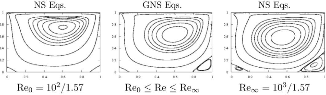
Figure 3 shows the contours plots of the steady solutions for the three type of fluids. Each flow consists of a core of fluid undergoing solid body rotation and small regions in the bottom corners of counter-rotating vortex. The intensity of the counter-rotating vortex is decreasing with respect to viscosity. The velocity profile along the vertical centerline is shown in Figure 4. We observe that, in the lower part of the cavity, the fluid is moving in contrary sense to the sense of the motion of the top wall. The maximum of the negative velocity depends decreasingly on the viscosity of the fluid.

NS Eqs. GNS Eqs. NS Eqs.

Re0 = 102/1.57 Re0 ≤Re≤Re∞ Re∞= 103/1.57

Figure 3: U = 0.01ms−1_{, a = 0.144. Contour plot of stream functions,}

steady solutions. Regular grid,51×51 grid points.

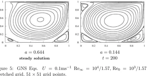
The second set of computations analyzes the response of the numerical method to the variation of the parameters of the fluid. The results are shown in Figure 5.

Final Remarks

Figure 4: U = 0.01ms−1, a = 0.144. Distribution of u-velocity along at vertical centre line of the cavity. Regular grid,51×51 grid points.

a= 0.644 a= 0.144

steady solution t= 200

Figure 5: GNS Eqs. U = 0.1ms−1 _Re

∞ = 104/1.57,Re0 = 103/1.57 .

Stretched grid, 51×51 grid points.

References

[1] P.D. Anderson, O.S. Galaktionov, G.W.M. Peters, F.N. van de Vose, H.E.H. Meijer. Mixing of non-Newtonian fluids in time-periodic cavity flow. J. Non-Newtonian Fluid Mech. 93:265-286, 2000.

[2] B. Andreianov, F. Boyer and F. Hubert. Finite volume scheme for the p-laplacian on cartezian meshes. M2AN. 38(6):931–960, 2004.

[3] J. Bell, P. Colella, and H. Glaz. A second-order projection method for in-compressible Navier-Stokes equations.J. Comp. Phys.85:257-283, 1989.

[4] K.L. Brenan, S.L. Campbell, L.R. Petzold.Numerical Solution of Initial Values Problems in Differential-Algebraic Equations.Classics in Applied Mathematics, SIAM, 1996.

[5] G.F. Carey, W. Barth, J. A. Woods, B. S. Kork, M. L. Anderson, S. Chow, and W. Bangerth. Modelling error and constitutive relations in simulattion of flow and transport. Int. J. Num. Meth. Fluids. 46:1211-1236, 2004.

[6] P. Carreau. Rheological equations from molecular network theories. Transactions of Society of Rheology. 16:99-127, 1972.

[7] A.J. Chorin. Numerical solution of the Navier-Stokes equations. Math. Comput.22:745-762, 1968.

[8] S.D. Cramer, J.M. Marchello. Numerical evolution of models describing non-Newtonian behavior. AIChE Journal.4(6):980-983, 1968.

[9] M.M. Cross. Rheology of non newtonian fluids: A new flow equation for pseudoplastic systems.Journal of Colloid and Interface Science. 20:417-437, 1965.

[10] R. Eymard, Th. Gallouet and R. Herbin. Finit Volume Method. In P.G. Ciarlet and J.L. Lions, (eds.) Handbook of Numerical Analysis. North Holland, 2000.

[12] J.L. Guermond, P. Minev, and Jie Shen. An overview of projection methods for incompressible flows. Comput. Methods Appl. Mech. En-grg. 195:6011-6045, 2006.

[13] F.H. Harlow and J.E. Welch. Numerical calculation of time-dependent viscous incompressible flow of fluid with free surface. Phys. Fluids. 8:2182-2189, 1965.

[14] J. Kim and P. Moin. Application of a fractional-step method to incom-pressible Navier-Stokes equations. J. Comp. Phys.59:308-323, 1985.

[15] S. Ion. Solving Generalized 2D Navier-Stokes Equations. Tech-nical report, Institute of Mathematical Statistics and Ap-plied Mathematics, Department of ApAp-plied Mathematics, 2009, http://www.ima.ro/publications/reports/rth_030605.pdf.

[16] O. A. Ladyzhenskaya.The Mathematical Theory of Viscous Incompress-ible Flow.Gordon and Breach, 1969.

[17] R. Temam.Navier–Stokes Equations. Elsevier Science, 1984.

[18] K. Yasuda, R.C. Armstrong, and R.E. Cohen. Shear flow properties of concentrated solutions of linear and star branched polystyrenes. Rheo-logica Acta. 20:163-178, 1981.

[19] K.K. Yeleswarapu. Evaluation of continuum models for characterizing the constitutive behavior of blood.Ph. D. thesis, University of Pittsburgh, 1996.