! " #$%&% '#()#*$'% ! + + ,
-*. /
0
!
" #
$%&' ( $%&'
)
The problem of flow inside a square cavity whose lid has constant velocity is solved. This problem is modeled by the Navier-Stokes equations. The numerical model is based on the finite volume method with numerical approximations of second-order accuracy and multiple Richardson extrapolations (MRE). The iterative process was repeated until the machine round-off error achievement. This work presents results for 42 variables of interest, and their discretization errors estimates, on the 1024 x 1024 nodes grid and the following Reynolds numbers: 0.01, 10, 100, 400 and 1000. These results are compared with sixteen sources in literature. The numerical solutions of this work are the most accurate obtained for this problem to date. The use of multiple Richardson extrapolations reduces the discretization error significantly.
Keywords: discretization error, error estimate, CFD, Richardson extrapolation, finite volume method
Introduction
1
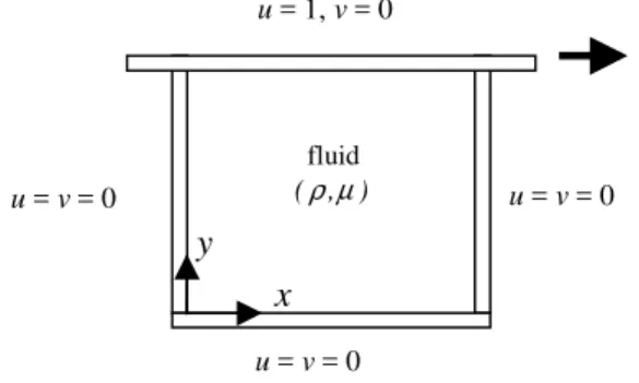
This work addresses the classical problem (Kawaguti, 1961; Burggraf, 1966; Rubin and Khosla, 1977; Benjamin and Denny, 1979; Ghia, Ghia and Shin, 1982) of laminar flow inside a square cavity of which lid moves at constant velocity: Fig. 1; where u and v are the components of the velocity vector in x and y directions, ρ and µ are fluid density and viscosity. This problem is widely employed to evaluate numerical methods and to validate codes for solving the Navier-Stokes equations (Botella and Peyret, 1998). In the works cited in Table 1, the problem was solved for 11 x 11 up to 2048 x 2048 node grids, and for Reynolds numbers (Re) from zero to 21,000.
Figure 1. Classical problem of the lid-driven square cavity flow.
As can be seen in Table 1, several numerical methods have been used, including finite difference method (FDM), finite volume method (FVM), finite elements method (FEM), lattice Boltzmann (LB), and the spectral method (Spectral). In addition, a variety of mathematical formulations has been used, including stream function and vorticity (ψ-ω); stream function and velocity (ψ-V); lattice Boltzmann equation (LBE), and the Navier-Stokes equations ( u-v-p). The problem considered here is also known as “singular driven
Paper accepted December, 2008. Technical Editor: Francisco R. Cunha
cavity” (Botella and Peyret, 1998), because there are two discontinuities in the boundary condition of u, at lid corners: 0 in one side and 1 in another. In contrast, there is a problem called “regularized driven cavity” (Botella and Peyret, 1998), which does not present discontinuities.
The main objective of this work is to present the most accurate numerical solutions found to date for the problem of “singular driven cavity” with Re = 0.01, 10, 100, 400 and 1000. To achieve this aim, we use the Navier-Stokes equations; the finite volume method; co-located arrangement of variables; segregated solution for the three conservation equations; numerical approximations of second-order accuracy; 1024 x 1024 control volumes uniform grid; the iterative process repeated until the machine round-off error achievement; double precision in calculations; and multiple Richardson extrapolations (Richardson, 1910). Solutions are presented for 42 variables of interest, which involve velocity profiles, mass flow rate, minimum value of the stream function, minimum and maximum velocities (and their coordinates), and wall forces on the fluid.
Other objectives of this work are: (1) propose an error estimator for use with numerical solutions obtained through multiple Richardson extrapolations; (2) verify (Roache, 1998) if the proposed estimator provides reliable error estimates for a problem of which analytical solution is known (Shih, Tan and Hwang, 1989); (3) apply the proposed estimator to each of the 42 variables of interest and five values of Re, presenting the estimated discretization error for each numerical solution; (4) confirm the order of accuracy (pL)
of the numerical solutions; and (5) compare the results with sixteen sources in literature. This work does not have as aim to present an optimized numerical model neither for CPU time nor for computational memory consumption. It is emphasized that the main objective is to provide the most accurate results to date for literature. Although there is extensive literature on the problem considered here, this work is justified by the following reasons:
No work appears to have been developed to date to estimate the numerical error involved in the solution of each variable of interest (Uh in Table 2). This is important, however, in order to know the
reliability of numerical solutions, allowing more careful comparisons to be made. Some authors have presented the solution variation for some variables for two or three grids; they, however,
x
y
u = v = 0 u = v = 0
u = v = 0
fluid
did not estimate numerical errors with any discretization error estimator.
Only Bruneau and Saad (2006) and Wright and Gaskell (1995) present solutions on grids as fine as those of the present work, but only for Re = 1000, few variables and without using multiple Richardson extrapolations. In Table 2, the column RE indicates whether the authors have used Richardson extrapolation or not; if the answer is positive, it is presented how many times it was used for each variable. In this work, it is going to be shown that RE reduces significantly the discretization error.
Most authors have stopped their iterative process (Ui) based on the residue criterion (R) or on the variation of any variable (Ferziger and Peric, 1999), with the tolerance value between 3 and 1.0e-12. In the present work, the iterative process is taken until the machine round-off error achievement.
In Table 2, “digits” represents the number of significant figures for each solution, which has the highest value in the presented work. In Table 2, pL is the theoretical accuracy of discretization error
of the approximations employed by each author. In the present work, the practical value obtained for this order is shown, for each variable of interest, confirming or not the theoretical value. In the next sections, the following subjects are discussed: the mathematical and numerical models; the theory and equations used to calculate effective and apparent orders of error to perform multiple Richardson extrapolations and the discretization error estimator; the results for the problem with known analytical solution; the classical problem results; and conclusions of this work.
Table 1. Author's formulation and grids for the classical problem.
Authors Ref. Formulation Re Method Grids
Kawaguti (1961) 1 ψ-ω 0 – 64 FDM 11 x 11
Burggraf (1966) 2 ψ-ω 0 – 700 FDM 11 x 11 – 51 x 51
Rubin and Khosla (1977) 3 ψ-ω 100 & 1,000 FDM etc 17 x 17 – 128 x 128
Benjamin and Denny (1979) 4 ψ-ω 1,000 – 10,000 FDM 61 x 61 – 151 x 151
Ghia, Ghia and Shin (1982) 5 ψ-ω 100 – 10,000 FDM 129 x 129 & 257 x 257
Schreiber and Keller (1983) 6 ψ-ω 1 – 10,000 FDM 121 x 121 – 180 x 180
Vanka (1986) 7 u,v,p 100 – 5,000 FDM 41 x 41 – 321 x 321
Hayase, Humphrey and Greif (1992) 8 u,v,p 100 – 10,000 FVM 10 x 10 – 80 x 80
Nishida and Satofuka (1992) 9 ψ-ω 100 – 3,200 FDM 65 x 65 & 129 x 129
Hou et al. (1995) 10 LBE 100 – 7,500 LB 256 x 256
Wright and Gaskell (1995) 11 u,v,p 100 & 1,000 FVM 1024 x 1024
Goyon (1996) 12 1,000 FDM 129 x 129
Barragy and Carey (1997) 13 ψ-ω 1.e-4 – 10,000 FEM 257 x 257
Botella and Peyret (1998) 14 u,v,p 100 & 1,000 Spectral 160
Zhang (2003) 15 ψ-ω 100 – 7,500 FDM 17 x 17 – 129 x 129
Erturk, Corke and Gökçöl (2005) 16 ψ-ω 1,000 – 21,000 FDM 401 x 401 – 601 x 601
Gupta and Kalita (2005) 17 ψ-V 100 – 10,000 FDM 41 x 41 – 161 x 161
Bruneau and Saad (2006) 18 u,v,p 1,000 – 10,000 FDM 128 x 128 – 2048 x 2048
This work (2008) 19 u,v,p 1.0e-2 – 1,000 FVM 2 x 2 – 1024 x 1024
Table 2. Author's numerical errors for the classical problem. Ref. p Precision Ui digits Uh RE
1 2 ? ? 5 ? No
2 2 single R: 5.0e-6 4 ? No
3 2 ? ? 3-4 ? No
4 2 ? ? 6 ? Yes = 1
5 2 ? R: 1.0e-4 5 ? No
6 2 ? ? 5 ? Yes = 3
7 2 ? R: 1.0e-3 4 ? No
8 2 ? R: 1.0e-5 ? ? No
9 2-10 ? R: 1.0e-8 6 ? No
10 1 single ? 4 8.7e-3 No
11 2 ? R: 1.0e-10 6 ? No
12 2 ? ? 4 ? No
13 8 ? R: 1.0e-6 5-7 1.0e-5 No
14 160 double R: 1.0e-8 7 1.0e-6 No
15 4 double ∆ψ,∆ω: 1.0e-4 6 ? No
16 2 ? R: 1.0e-10 6 ? Yes = 2
17 2 ? ∆ψ: 5.0e-7 3 ? No
18 3 ? 1.0e-12 5 ? No
Nomenclature
E = true discretization error
F = viscous drag force of the cavity’s lid or wall on the fluid in x direction (N)
h = size of the control volumes (m) m = number of Richardson extrapolation M = mass flow rate (kg/s)
nm = number of grids p = pressure (Pa)
pE = effective order of the discretization error
pL = asymptotic order of the discretization error
pU = apparent order of the discretization error
r = grid refinement ratio Re = Reynolds number S = source term in Eq. (3)
u = component of the velocity vector in the x direction (m/s) U = estimated discretization error
v = component of the velocity vector in the y direction (m/s) x = Cartesian coordinate in the horizontal direction (m) y = Cartesian coordinate in the vertical direction (m) z = depth of the cavity (m)
Greek symbols
φ = numerical solution of the variable of interest
Φ = exact analytical solution of the variable of interest
µ = viscosity (Pa.s)
ρ = density (kg/m3)
ψ = stream function (m2/s) Subscripts
1 fine grid 2 coarse grid 3 supercoarse grid
Mathematical Model
The mathematical model of the problem consists of the Conservation of Mass and the Conservation of Momentum laws (the Navier-Stokes equations). Simplifications considered for the problem are: steady state; two-dimensional laminar flow in x and y directions; incompressible fluid; µ as constant; and absence of other effects. Thus, the resulting mathematical model is:
0 = ∂ ∂ + ∂ ∂ y v x u (1) x p y u x u y uv x u ∂ ∂ − ∂ ∂ + ∂ ∂ µ = ∂ ∂ ρ + ∂ ∂ ρ 2 2 2 2 2 ) ( ) ( (2) S y p y v x v y v x uv + ∂ ∂ − ∂ ∂ + ∂ ∂ µ = ∂ ∂ ρ + ∂ ∂ ρ 2 2 2 2 2 ) ( ) ( (3)
where p is the pressure and S is a source term, which is null at the classical problem (without known analytical solution) and given by Shih, Tan and Hwang (1989) in the case of a manufactured solution problem. The domain is a square of unitary side with the origin of the system of coordinates, as shown in Fig. 1.
The variables of interest of the problem involve the primitive variables themselves (u and v) and integrations of u and v, which are:
Profile of u in x = ½ at 15 selected points of y.
Profile of v in y = ½ at 15 selected points of x.
The minimum value (umin) of profile of u in x = ½ and its
respective y coordinate.
The minimum (vmin) and the maximum (vmax) values of profile of
v in y = ½ and their respective x coordinates.
The minimum value of the stream function (ψmin) and its
coordinates x and y.
The mass flow rate (M) that flows through y = ½ line between x = 0 and ½ , i.e.,
∫
ρ
==
12 2 10
v
z
dx
M
y (4)where z is the cavity depth, which is considered unitary.
The viscous drag force (F) in direction x (Hou et al., 1995) is the force exerted by the fluid boundary surface, calculated by
∫
∂
∂
µ
=
10
y
z
dx
u
F
y
(5)
where Fn is F in y = 1 (cavity movable lid) and Fs is F in y = 0 (the
lower cavity wall).
Numerical Model
Briefly, the numerical model adopted to solve the mathematical model described by Eqs. (1) to (3) has the following characteristics: (1) finite volume method (Ferziger and Peric, 1999); (2) central difference scheme (CDS) (Ferziger and Peric, 1999) for diffusive and pressure terms; (3) CDS scheme with deferred correction (Ferziger and Peric, 1999; Khosla and Rubin, 1974) on upstream difference scheme (UDS) for advective terms; (4) Eqs. (1) to (3) are solved sequentially using the MSI (Modified Strongly Implicit) method (Schneider and Zedan, 1981); (5) SIMPLEC (Semi IMPlicit Linked Equations Consistent) method (Van Doormaal and Raithby, 1984) to treat the pressure-velocity coupling; (6) uniform grids; (7) the boundary conditions for u and v, Fig. 1, are applied employing ghost volumes (Ferziger and Peric, 1999); (8) Eqs. (1) to (3) are written for unsteady state, aiming the use of time as a relaxation parameter in the iterative solution process of the discretized mathematical model; and (9) a co-located arrangement of variables is used (Marchi and Maliska, 1994). This numerical model does not require boundary conditions for pressure (Ferziger and Peric, 1999). The numerical solution of the variables of interest is obtained as follows:
• The numerical solution of the profile of u in x = ½ is obtained by the mathematical average of u stored at the east face of the two adjacent volumes to each desired y coordinate. This u at each control volume east face is that one of the co-located arrangement of variables of Marchi and Maliska (1994). This is necessary because the number of volumes used in each coordinate direction is even, so that no control volume center coincides with the line x = ½.
• The numerical solution of the profile of v in y = ½ is obtained analogously to the profile of u, through the mathematical average of v stored at the north face of the two adjacent volumes to each desired x coordinate.
• umin is the minimum value of the solution of u stored at east
faces among all control volumes of the grid with x = ½. And its y coordinate is the one in the east face center of the volume corresponding to umin.
• vmin and vmax are the minimum and the maximum values of the
the north face center of the volumes corresponding to vmin and
vmax.
• For each vertical line, numerical solution of the stream function field (ψ) is obtained through integration of the product of u, stored at each control volume east face, by the height of each control volume (∆y), starting from the lower wall, in y = 0. The vertical lines coincide with x coordinates of the faces of each control volume. The numerical integration used here is based on the rectangular rule (Kreyszig, 1999). The minimum value of the stream function (ψmin) is obtained directly from the ψ field. • The numerical solution of the mass flow rate (M) defined by Eq.
(4) is obtained by numerical integration employing the rectangular rule, through
∑
= =
∆ ρ
= /2
1 , , 12
X N i y i n v x z M (6)
where i represents the number of the control volume in x direction; i = 1 is the real control volume at the left-hand wall of the cavity; Nx is the total number of real control volumes in x
direction; ∆x is the width of each control volume; and vn is v at
the north face of each control volume.
• The numerical solution of the force (Fn), which is defined by Eq. (5), is obtained with one upstream point (UDS) (Ferziger and Peric, 1999) and the numerical integration used here is the rectangular rule, which results in
∑
= − ∆ ∆ µ= X Y
N i N i i T u u y x z Fn 1 , , ) ( 2 (7)
where uT,i is the velocity of the cavity lid at the x coordinate of
each control volume i center; and
Y N i
u, is the nodal velocity u at each real i control volume center, whose volume north face coincides with the cavity lid.
• The numerical solution of Fs, defined by Eq. (5), is obtained analogously to Fn but with one point downstream (DDS) (Ferziger and Peric, 1999), resulting in
∑
= ∆ ∆ µ −= NX
i i u y x z Fs 1 1 , 2 (8)
where ui,1 is the nodal velocity u at each real i control volume center, whose volume south face coincides with the cavity lower wall, whose u = 0.
The Stokes 1.5 computational code was implemented in Fortran 95, using Intel Fortran 9.1 compiler and double precision. The iterative process is repeated until the machine round-off error achievement. This is verified by monitoring the l1-norm (Kreyszig, 1999), along the iterations, of the residue (R) sum of the three solved systems of Eqs. (1) to (3). The residue sum value of the three systems, in each outer iteration, is nondimensionalized by its value at the end of the first outer iteration (R1).
Discretization Error
The numerical error (E) can be defined as the difference between the exact analytical solution (Φ) of a variable of interest and its numerical solution (φ), i.e.,
φ − Φ = φ) ( E (9)
The sources that cause numerical error can be split into four types (Marchi and Silva, 2002): truncation, iteration, round-off, and programming errors. When other sources of error are inexistent or much smaller in relation to truncation ones, the numerical error can also be called as discretization error.
Considering the numerical model described in the previous section, the predicted asymptotic order (pL) of the discretization
error is equal to two (Ferziger and Peric, 1999; Schneider, 2007) for all variables of interest, except for x and y coordinates of ψmin, umin,
vmin and vmax, of which pL are unknown. In literature (Roache, 1998,
1994), pL is also called formal order or accuracy order.
In theory (Marchi, 2001), it is expected that pE (effective order)
and pU (apparent order) → pL for h → 0. In other words, it is
expected that the practical orders (pE and pU), which are calculated
with the numerical solutions of each variable of interest, tend toward the asymptotic order (pL), foreseen a priori, when the size of the
control volumes (h) tends toward zero.
The effective order (pE) of the true error is defined by (Marchi,
2001) ) log( ) ( ) ( log 1 2 r E E pE φ φ = (10)
where E(φ1) and E(φ2) are true discretization errors of the numerical solutions φ1 and φ2 obtained, respectively, with fine (h1) and coarse (h2) grids; h = size of the control volumes (in this work, h = ∆x =
∆y); and r = h2/h1 (grid refinement ratio).
According to Eq. (10), the effective order (pE) is function of the
true discretization error of a variable of interest. Thus, for problems which analytical solution is known, it can be used to verify a posteriori if, as h→ 0, one obtains pL. When E is unknown, (pE)
cannot be calculated. In this case, one can use the concept of observed or apparent order (pU) defined by (De Vahl Davis, 1983;
Marchi and Silva, 2002)
) r log( log pU − −
= 1 2
3 2 φ φ φ φ (11)
where φ1, φ2 and φ3 = numerical solutions obtained, respectively, with fine (h1), coarse (h2) and supercoarse (h3) grids, and r = h3/h2 = h2/h1.
Some studies (Benjamin and Denny, 1979; Schreiber and Keller, 1983; Erturk, Corke and Gökçöl, 2005) achieved excellent results when employing multiple Richardson extrapolations (MRE) to reduce the discretization error of ψmin. However, these authors used
this process with at most four grids, resulting in up to three extrapolations for the finest grid they used. In the present work, this procedure was utilized with up to ten grids, resulting in up to nine extrapolations for the finest grid used (1024 x 1024), and applied to almost all variables of interest. This was done by means of
) nm ..., , , m ( , rpV(m)
) m ( , ) m ( , ) m ( , m , 1 2 1 1 1 2 1 1 1 1 1 − = − − + = − ∞ − ∞ − ∞
∞ φ φ φ
φ (12)
different grids with numerical solutions of φ without any extrapolation; pV(m) = true orders (Marchi and Silva, 2002) of the
discretization error, with pV(1) = pL. For the numerical model used
in this work, pV = 2, 4, 6 ... for all variables of interest, except for x
and y coordinates of ψmin, umin, vmin and vmax, of which values of pV
are unknown.
In this work, Eq. (12) is applied to all variables of interest to reduce the discretization error, except to x and y coordinates of ψmin,
umin, vmin and vmax, of which results are the ones obtained with the
finest grid, of 1024 x 1024 nodes, without any extrapolation. In theory, the accuracy order of the results of u(0.5;05), v(0.5;0.5), M, Fs, Fn, vmin, vmax, umin and ψmin is 20, since they are obtained with
nine extrapolations through Eq. (12). And, in the case of the profiles of u and v, it is 14, because they are obtained with six extrapolations.
In practical situations, a numerical solution is obtained because the analytical solution is unknown. Hence, the true value of the numerical error is also unknown. Therefore, the numerical error must be estimated. The estimated discretization error (U) of
∞ −
φ1,(nm1) , i.e., of the numerical solution with the highest possible number of extrapolations in the finest grid, will be considered equal to
∞ − ∞ − ∞
− =φ −φ
φ1,( 1) ) 1,( 2) 2,( 2)
( nm nm nm
U (13)
which is the module of the difference with the highest number of extrapolations that can be calculated between the two finest grids. In the case of the x and y coordinates of ψmin, umin, vmin and vmax, one
adopts
512 512 1024 1024
)
,
(
x
y
x xU
=
φ
−
φ
(14)where φ1024x1024 and φ512x512 are the numerical solutions obtained without extrapolation on 1024 x 1024 and 512 x 512 nodes grids.
Literature (Roache, 1998) offers several discretization error estimators. The use of Eqs. (13) and (14) is justified based on an analysis of the problem presented in the next section. This problem is similar to the classical problem of square cavity with movable lid, but its analytical solution is known. Thus, it was possible to evaluate the performance of Eqs. (13) and (14), which resulted in reliable error estimates, i.e., U/|E| ≥ 1 for all variables of interest of the present work.
Problem with Known Analytical Solution
There is a variant of the classical problem of which analytical solution is known and is given by Shih, Tan and Hwang (1989). In this case, the source term (S) of Eq. (3) is different from zero, and is
presented in Shih, Tan and Hwang (1989). The analytical solution of u and v is (Shih, Tan and Hwang, 1989)
) 2 4 ( ) 2 ( 8 ) ,
( 4 3 2 3
y y x x x y x
u = − + − (15)
) ( ) 2 6 4 ( 8 ) ,
( 3 2 4 2
y y x x x y
x
v =− − + − (16)
The lid velocity varies with x, according to Eq. (15) for y = 1. The other boundary conditions are shown in Fig. 1. The Reynolds number (Re) is one for Eq. (17).
All numerical solutions in this work were obtained with ten different grids: 2 x 2, 4 x 4, 8 x 8 and so on up to 1024 x 1024 real control volumes. All simulations of this study were made in a Xeon Quad Core X5355 Intel processor, 2.66 GHz, using one core. The maximum RAM memory employed was 242 MB, for the simulations with 1024 x 1024 nodes grid. To obtain the numerical solutions, the initial estimate used for u, v and p was the analytical one for the problem given, respectively, by Eqs. (15) and (16) and by Shih, Tan and Hwang (1989).
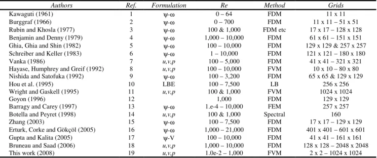
The column named as Shih, in Table 3, presents the main parameters of the iterative process involved in the problem solution for the 1024 x 1024 nodes grid. At this table: ∆t is the time interval used to further the iterative process; Itmax is the total number of outer iterations made; It(Eπ) is the approximate number of outer iterations made when the round-off error level is achieved; R1 is the l1-norm of the residue sum of the three solved systems after the first iteration; Rf/R1 is the l1-norm of the residue sum of the three solved systems at Itmax, made dimensionless based on the first iteration, showing how much the residue was reduced along the iterative process; Alg is the number of significant figures of the solution which does not have round-off errors after Itmax iterations; and tCPU is the CPU time needed to make Itmax iterations. The typical behavior of the residue drop along the iterations and the machine round-off error achievement are shown in Fig. 2 for the 256 x 256 nodes grid. In that figure, Shih denotes the problem from this section, and Ghia the problem treated in the next section.
Ideally, for the model used in this work, the value of the stream function (ψ) in y = 1 should be null for each of the 1024 control volumes at the cavity lid. Its absolute maximum value, which represents the mass conservation error, resulted in 1.4 x 10⁻¹⁴; which is very near the null value and is at the level of double precision used in this work.
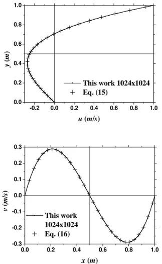
The velocity profiles in the two directions in the cavity center are shown in Fig. 3. The congruence between the analytical solution of Shih, Tan and Hwang (1989) and the numerical solution of the present work, with the 1024 x 1024 grid, can be considered excellent.
Table 3. Parameters of the iterative process for the 1024 x 1024 nodes grid.
Shih --- The classical problem --- Variable
Re = 1 Re = 0.01 Re = 10 Re = 100 Re = 400 Re = 1000
∆t (s) 5.0e-4 1.0e-5 0.02 0.05 0.5 0.5
Itmax 60,000 200,000 380,000 100,000 240,000 100,000
It(Eπ) 45,000 150,200 362,700 80,900 202,300 85,300
R1 3.8e-01 1.0e+04 1.6e+02 1.2e+02 1.2e+02 1.2e+02
Rf/R1 2.8e-10 9.5e-13 5.9e-14 8.1e-15 3.3e-15 1.6e-15
Alg 7(v) e 12 10 12 12 13 12
0 1x10⁴ 2x10⁴ 3x10⁴ 10-16
10-14
10-12 10-10 10-8 10-6 10-4
10-2 100
l1
-n
o
rm
R
f/
R
1
Iterations
Shih, Re=1 Ghia, Re=0.01 Ghia, Re=10 Ghia, Re=100 Ghia, Re=400 Ghia, Re=1,000
Figure 2. Residue versus iterations for the 256 x 256 nodes grid.
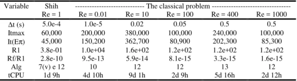
Table 4. Results for the problem of Shih, Tan and Hwang (1989).
Variable pE φ E U/|E|
ψmin 1.956996 -1.2500000e-1 2.0e-9 2.4e+2
x(ψmin) Ind. 5.0e-1 0 Ind.
y(ψmin) 0 7.0703e-1 7.6e-5 6.4
M 2.000252 9.3749999997e-2 2.7e-12 7.4
Fs 1.999764 5.333333334e-1 -8.2e-11 1.8e+1
Fn 1.638635 2.666678e+0 -1.1e-5 3.1
umin 2.082329 -2.721659e-1 3.4e-7 1.1e+1
y(umin) 1.071713 4.0869e-1 -4.4e-4 1.1
vmin 2.583567 -2.886756e-1 4.2e-7 2.6
x(vmin) 2.545598 7.8857e-1 1.0e-4 4.9
vmax 2.566173 2.886756e-1 -4.2e-7 2.6
x(vmax) 2.545598 2.1143e-1 -1.0e-4 4.9
u(0.5;0.0625) 2.000029 -6.2011718741e-2 -8.5e-12 7.3
u(0.5;0.125) 2.000029 -1.21093749988e-1 -1.2e-11 7.3
u(0.5;0.1875) 2.000077 -1.74316406238e-1 -1.2e-11 7.4
u(0.5;0.25) 1.999877 -2.18749999990e-1 -9.8e-12 7.3
u(0.5;0.3125) 1.999951 -2.51464843745e-1 -5.4e-12 7.6
u(0.5;0.375) 1.999963 -2.695312499997e-1 -2.8e-13 1.8e+1
u(0.5;0.4375) 1.999966 -2.70019531254e-1 4.0e-12 6.2
u(0.5;0.5) 1.999965 -2.50000000006e-1 5.9e-12 6.6
u(0.5;0.5625) 1.999963 -2.06542968755e-1 4.6e-12 6.7
u(0.5;0.625) 1.999960 -1.367187500006e-1 6.0e-13 6.7
u(0.5;0.6875) 1.999961 -3.7597656248e-2 -2.0e-12 6.5
u(0.5;0.75) 1.999970 9.3749999998e-2 2.0e-12 9.0
u(0.5;0.8125) 1.999986 2.60253906243e-1 7.2e-12 7.8
u(0.5;0.875) 2.000027 4.64843749987e-1 1.3e-11 7.5
u(0.5;0.9375) 1.995103 7.10449218737e-1 1.3e-11 7.0
v(0.0625;0.5) 1.999920 1.53808593744e-1 6.2e-12 7.1
v(0.125;0.5) 1.999929 2.4609374999e-1 1.4e-11 7.1
v(0.1875;0.5) 1.999935 2.8564453123e-1 1.5e-11 7.3
v(0.25;0.5) 1.999942 2.81249999990e-1 1.0e-11 7.6
v(0.3125;0.5) 1.999952 2.41699218747e-1 3.3e-12 7.6
v(0.375;0.5) 1.999964 1.75781250002e-1 -2.3e-12 6.5
v(0.4375;0.5) 1.999979 9.2285156254e-2 -3.7e-12 6.8
v(0.5;0.5) 1.999762 2.3e-14 -2.3e-14 1.0e+1
v(0.5625;0.5) 1.999963 -9.2285156254e-2 3.6e-12 6.9
v(0.625;0.5) 1.999959 -1.75781250002e-1 2.1e-12 6.2
v(0.6875;0.5) 1.999952 -2.41699218746e-1 -3.5e-12 7.7
v(0.75;0.5) 1.999944 -2.81249999989e-1 -1.1e-11 7.0
v(0.8125;0.5) 1.999938 -2.8564453123e-1 -1.5e-11 7.3
v(0.875;0.5) 1.999934 -2.4609374999e-1 -1.4e-11 7.1
0.0 0.2 0.4 0.6 0.8 1.0
-0.2 0.0 0.2 0.4 0.6 0.8 1.0
u (m/s)
y
(m
)
This work 1024x1024
Eq. (15)
0.0 0.2 0.4 0.6 0.8 1.0
-0.3 -0.2 -0.1 0.0 0.1 0.2 0.3
v
(m
/s
)
x (m)
This work
1024x1024
Eq. (16)
Figure 3. u at x = ½ and v at y = ½ for the problem of Shih, Tan and Hwang (1989).
For each variable of interest, Tab. 4 presents: (a) the effective order (pE) calculated by Eq. (10), based on the true discretization
error (E) of the numerical solutions (φ) without extrapolation, on the 1024 x 1024 and 512 x 512 nodes grids, i.e., with r = 2; (b) the numerical solution (φ) on the 1024 x 1024 nodes grid, with extrapolation calculated by Eq. (12), except for x and y variables for which none extrapolation was employed; (c) the value of E calculated by Eq. (9); and (d) the ratio of the estimated discretization error (U) to the module of E. In this table and in the following ones, the notation 1.0e-3 and Ind. represent, respectively, 1.0 x 10⁻³ and indefinite.
In Tab. 4, it can be noted that for the velocity profiles of u and v, pE varies from 1.995 to 2.000, confirming the value of pL = 2,
which was predicted a priori. For coordinate type variables, pE is
indefinite or assumes values of null and close to unity or to two. For other variables, pE varies from 1.639 to 2.584, i.e., around pL.
Table 4 indicates, for all variables of interest, that U/|E| ≥ 1 for U calculated by Eqs. (13) or (14) depending on the variable. In other words, the analytical solution is contained within the interval comprised by φ±U. For the velocity profiles u and v, the U/|E| ratio varies between 6.2 and 18. For coordinate type variables, this ratio varies from 1.1 to 6.4. For other variables, the ratio varies between 2.6 and 240.
For the velocity profiles u and v, M and Fs, the |Eh/E| ratio varies from 1.6 x 10³ to 3.8 x 10⁶. This ratio represents the extension to which the discretization error of the solution without extrapolation (Eh), obtained on the 1024 x 1024 grid, is reduced with the use of multiple extrapolations through Eq. (12). This reduction was not so effective for the variables vmin, vmax, umin, Fn
and ψmin, which reductions were, respectively, of 1.9, 2.0, 2.6, 4.6
and 75.
The magnitude of E and U may vary considerably along the velocity profiles. The ratio between the maximum and the minimum values of E is 652, and for U it is 478.
Summarizing, in this section, for a two-dimensional flow problem with known analytical solution, we showed: (1) the importance of using multiple extrapolations to reduce the true discretization error (E); and (2) the discretization error estimated (U) with Eq. (13) or (14) reliability, i.e., U/|E| ≥ 1. In the next section, the same procedure is applied to the classical cavity flow problem of which analytical solution is unknown.
Classical Problem with Unknown Analytical Solution
In the classical problem (Kawaguti, 1961; Burggraf, 1966; Rubin and Khosla, 1977; Benjamin and Denny, 1979; Ghia, Ghia and Shin, 1982) of laminar flow inside a square cavity, the lid velocity (UT) is constant and has unitary value. The other boundary
conditions are shown in Fig. 1. At lid corners, u = 0 on one side and u = 1 on the other. The source term (S) of Eq. (3) is null. The Reynolds number (Re) is defined by
µ ρ
= UT L
Re (17)
where L = 1 m, dimension of the side of the square cavity; ρ = 1 kg/m3, density; and µ is the viscosity in Pa.s, obtained from Eq. (17) for a given Re. Numerical solutions were obtained for Re = 0.01, 10, 100, 400 and 1000. The initial estimate used was u = v = p = 0.
Table 3 shows the main parameters of the iterative process involved in the problem solution achievement for the 1024 x 1024 nodes grid. It is noted that the typical behavior of the residue drop along iterations and the achievement of the machine round-off error are shown in Fig. 2 for the 256 x 256 nodes grid. For these five values of Re and the 1024 x 1024 grid, CPU time varied from 2 days and 9 hours to 9 days and 1 hour. The l1-norm of the residue sum of the three solved systems varied from 1.6 x 10⁻¹⁵ to 9.5 x 10⁻¹³. The obtained solutions present from 10 to 13 significant figures without machine round-off error.
The stream function value (ψ) in y = 1, which should be null for each of the 1024 control volumes at the cavity lid, resulted in the following maximum values: 5.9 x 10⁻¹⁶, 1.7 x 10⁻¹⁵, 5.4 x 10⁻¹⁶, 1.0 x 10⁻¹⁵ and 2.3 x 10⁻¹⁵, respectively, for Re = 0.01, 10, 100, 400 and 1000. These values are very close to the null one, being at the level of double precision employed in this work.
0.0 0.2 0.4 0.6 0.8 1.0
-0.4 -0.2 0.0 0.2 0.4 0.6 0.8 1.0
Re =
0.01 and 10
100
400
1000
u (m/s)
y
(m
)
This work 1024x1024 Botella and Peyret (1998) Bruneau and Saad (2006) Ghia, Ghia and Shin (1982)
0.0 0.2 0.4 0.6 0.8 1.0
-0.4 -0.2 0.0 0.2 0.4
1000 1000
400 400
100 100
0.01 and 10 0.01 and 10
Re =
v
(m
/s
)
x (m)
This work 1024x1024 Botella and Peyret (1998) Bruneau and Saad (2006) Ghia, Ghia and Shin (1982)
Figure 4. u at x = ½ and v at y = ½ for the classical problem.
Table 5. Apparent order (pU) for the classical problem.
Variable Re = 0.01 Re = 10 Re = 100 Re = 400 Re = 1000
ψmin 1.813490 1.329414 1.831320 2.001399 1.995930
x(ψmin) Ind. Ind. Ind. Ind. Ind.
y(ψmin) Ind. Ind. Ind. Ind. Ind.
M 2.034916 2.028581 1.996948 2.006947 2.002034
Fs 1.992172 1.994006 2.029269 1.332492 1.929611
Fn -1.59e-6 -9.89e-5 -3.50e-4 5.21e-3 3.06e-2
umin 2.181172 2.066232 2.075970 2.031114 1.997271
y(umin) 1 1 Ind. Ind. Ind.
vmin 1.621232 2.190969 1.101600 2.143075 2.125597
x(vmin) Ind. 1 Ind. Ind. 1
vmax 1.634400 1.868090 1.997206 2.016770 1.972962
x(vmax) Ind. Ind. Ind. Ind. Ind.
u(0.5;0.0625) 1.960768 1.968367 2.147456 1.984548 1.976726
u(0.5;0.125) 1.958143 1.964883 1.868924 1.999443 1.993667
u(0.5;0.1875) 1.923552 1.931919 1.978974 2.004525 2.005013
u(0.5;0.25) 2.178329 2.126091 1.993379 2.007160 2.015676
u(0.5;0.3125) 2.031881 2.026274 1.998071 2.009989 2.014781
u(0.5;0.375) 2.015371 2.013097 2.000054 2.014118 2.017440
u(0.5;0.4375) 2.008997 2.007837 2.000902 2.020004 2.027410
u(0.5;0.5) 2.005441 2.004812 2.000935 2.028634 2.071716
u(0.5;0.5625) 2.002936 2.002602 1.999763 1.988412 1.932956
u(0.5;0.625) 2.000757 2.000613 1.995031 2.003845 1.981615
u(0.5;0.6875) 1.998272 1.998354 2.085979 2.006704 1.991411
u(0.5;0.75) 1.993929 1.994724 2.004496 2.007500 1.996045
u(0.5;0.8125) 1.976978 1.980210 1.996234 2.007477 1.999568
u(0.5;0.875) 2.057222 2.046188 1.986320 2.007307 2.002394
u(0.5;0.9375) 2.019786 2.017118 1.986999 2.009975 2.010322
v(0.0625;0.5) 2.218522 2.029222 1.990425 2.004249 2.005623
v(0.125;0.5) 2.025451 2.012204 1.991731 2.005891 2.004193
v(0.1875;0.5) 2.011352 2.007024 1.993743 2.006560 2.003540
v(0.25;0.5) 2.006277 2.004850 1.996269 2.007214 2.000912
v(0.3125;0.5) 2.003755 2.004056 1.999362 2.007830 1.996139
v(0.375;0.5) 2.002376 2.004485 2.003797 2.007450 1.991814
v(0.4375;0.5) 2.001669 2.008224 2.014244 1.901847 1.978584
v(0.5;0.5) 1.973113 1.972879 1.759938 2.013626 2.345369
v(0.5625;0.5) 2.001658 1.996774 1.981704 2.010731 2.027308
v(0.625;0.5) 2.002371 1.999829 1.992687 2.008691 2.015160
v(0.6875;0.5) 2.003753 2.002233 1.997319 2.007301 2.010284
v(0.75;0.5) 2.006278 2.005644 2.000465 2.005482 2.006818
v(0.8125;0.5) 2.011358 2.012787 2.003962 2.003772 2.009697
v(0.875;0.5) 2.025481 2.043456 2.080131 2.007310 2.004484
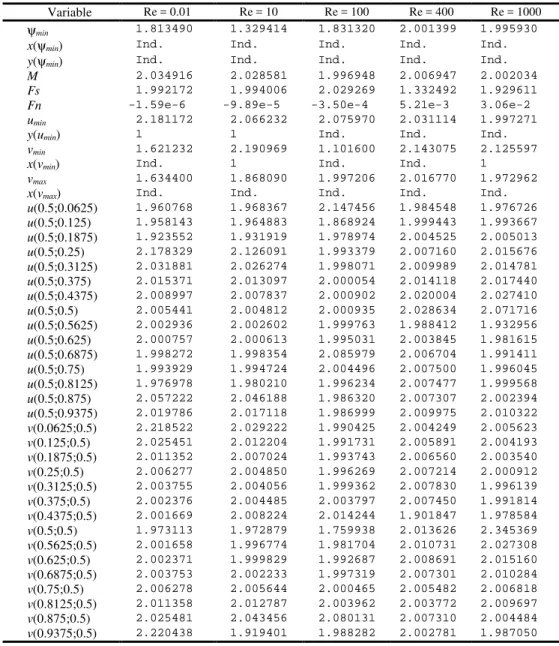
Table 5 presents the apparent order (pU) for Re = 0.01, 10, 100,
400 and 1000. This order was calculated using Eq. (11), based on the numerical solutions (φ) of each variable of interest, without extrapolation, on the 1024 x 1024, 512 x 512 and 256 x 256 nodes grids, i.e., with r = 2. For the u and v velocity profiles, pU varies from
1.760 to 2.345, with most results very close to the value of pL = 2,
which was predicted a priori. For coordinate type variables, pU is
indefinite or assumes a unitary value. For other variables, pU can differ
substantially from pL, varying from 1.102 to 2.191.
An unexpected behavior of pU, shown in Table 5, occurred for the
variable Fn. For all five values of Re, pU varies between -3.50 x 10⁻⁴
and 3.06 x 10⁻². Based on pU versus h curves, it was found that pU→ 0
for h → 0. This means that the value of Fn diverges with grid refinement. In Nie, Robbins and Chen (2006), for the same problem studied in this work, it was shown that Fn cannot be obtained solely through continuum mechanics, i.e., with the Navier-Stokes equations. It is also necessary to consider the movement on microscopic scale. This problem is due to the discontinuity existing in the boundary
condition of u, at lid corners: 0 on one side and 1 on the other. In Bruneau and Saad (2006), two other variables were found to diverge when h → 0, due to the discontinuity existing in the boundary condition of u. It should be noted that for Fs: (a) in all five values of Re, its value converges to h→ 0; (b) it is calculated with the same types of numerical approximations as Fn; (c) its pU varies from
1.322 to 2.029; and (d) its calculation does not involve discontinuities.
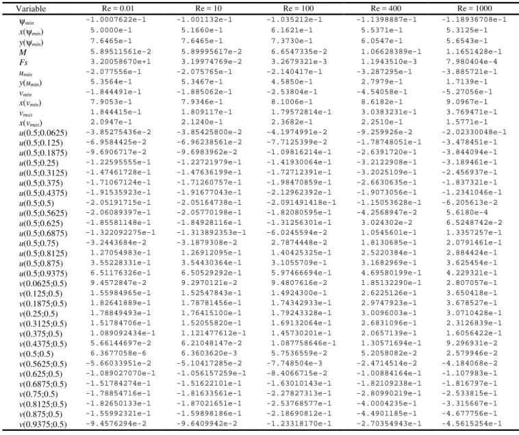
Table 6 presents, for Re = 0.01, 10, 100, 400 and 1000, the numerical solution (φ) of each variable of interest. In the case of coordinate type variables, the solution is presented without extrapolations, obtained on the 1024 x 1024 nodes grid. For the remaining variables, the solution is the one obtained on the 1024 x 1024 nodes grid with extrapolations through Eq. (12). No results are shown for Fn due to its divergence. The number of significant figures presented for each variable is defined by its respective U value from Table 7.
Table 6. Numerical solution (φφφφ) for the classical problem.
Variable Re = 0.01 Re = 10 Re = 100 Re = 400 Re = 1000
ψmin -1.0007622e-1 -1.001132e-1 -1.035212e-1 -1.1398887e-1 -1.18936708e-1
x(ψmin) 5.0000e-1 5.1660e-1 6.1621e-1 5.5371e-1 5.3125e-1
y(ψmin) 7.6465e-1 7.6465e-1 7.3730e-1 6.0547e-1 5.6543e-1
M 5.89511561e-2 5.89995617e-2 6.6547335e-2 1.06628389e-1 1.1651428e-1
Fs 3.20058670e+1 3.19974769e-2 3.2679321e-3 1.1943510e-3 7.980404e-4
umin -2.077556e-1 -2.075765e-1 -2.140417e-1 -3.287295e-1 -3.885721e-1
y(umin) 5.3564e-1 5.3467e-1 4.5850e-1 2.7979e-1 1.7139e-1
vmin -1.844491e-1 -1.885062e-1 -2.53804e-1 -4.54058e-1 -5.27056e-1
x(vmin) 7.9053e-1 7.9346e-1 8.1006e-1 8.6182e-1 9.0967e-1
vmax 1.844415e-1 1.809117e-1 1.79572814e-1 3.0383231e-1 3.769471e-1
x(vmax) 2.0947e-1 2.1240e-1 2.3682e-1 2.2510e-1 1.5771e-1
u(0.5;0.0625) -3.85275436e-2 -3.85425800e-2 -4.1974991e-2 -9.259926e-2 -2.02330048e-1
u(0.5;0.125) -6.9584425e-2 -6.96238561e-2 -7.7125399e-2 -1.78748051e-1 -3.478451e-1
u(0.5;0.1875) -9.6906717e-2 -9.6983962e-2 -1.09816214e-1 -2.6391720e-1 -3.844094e-1
u(0.5;0.25) -1.22595555e-1 -1.22721979e-1 -1.41930064e-1 -3.2122908e-1 -3.189461e-1
u(0.5;0.3125) -1.47461728e-1 -1.47636199e-1 -1.72712391e-1 -3.2025109e-1 -2.456937e-1
u(0.5;0.375) -1.71067124e-1 -1.71260757e-1 -1.98470859e-1 -2.6630635e-1 -1.837321e-1
u(0.5;0.4375) -1.91535923e-1 -1.91677043e-1 -2.12962392e-1 -1.9073056e-1 -1.2341046e-1
u(0.5;0.5) -2.05191715e-1 -2.05164738e-1 -2.091491418e-1 -1.15053628e-1 -6.205613e-2
u(0.5;0.5625) -2.06089397e-1 -2.05770198e-1 -1.82080595e-1 -4.2568947e-2 5.6180e-4
u(0.5;0.625) -1.85581148e-1 -1.84928116e-1 -1.31256301e-1 3.024302e-2 6.5248742e-2
u(0.5;0.6875) -1.322092275e-1 -1.313892353e-1 -6.0245594e-2 1.0545601e-1 1.3357257e-1
u(0.5;0.75) -3.2443684e-2 -3.1879308e-2 2.7874448e-2 1.8130685e-1 2.0791461e-1
u(0.5;0.8125) 1.27054983e-1 1.26912095e-1 1.40425325e-1 2.5220384e-1 2.884424e-1
u(0.5;0.875) 3.55228331e-1 3.54430364e-1 3.1055709e-1 3.1682969e-1 3.625454e-1
u(0.5;0.9375) 6.51176326e-1 6.50529292e-1 5.97466694e-1 4.69580199e-1 4.229321e-1
v(0.0625;0.5) 9.4572847e-2 9.2970121e-2 9.4807616e-2 1.85132290e-1 2.807057e-1
v(0.125;0.5) 1.55984965e-1 1.52547843e-1 1.4924300e-1 2.6225126e-1 3.650418e-1
v(0.1875;0.5) 1.82641889e-1 1.78781456e-1 1.74342933e-1 2.9747923e-1 3.678527e-1
v(0.25;0.5) 1.78849493e-1 1.76415100e-1 1.79243328e-1 3.0096003e-1 3.0710428e-1
v(0.3125;0.5) 1.51784706e-1 1.52055820e-1 1.69132064e-1 2.6831096e-1 2.3126839e-1
v(0.375;0.5) 1.089092434e-1 1.121477612e-1 1.45730201e-1 2.0657139e-1 1.6056422e-1
v(0.4375;0.5) 5.66144697e-2 6.21048147e-2 1.087758646e-1 1.30571694e-1 9.296931e-2
v(0.5;0.5) 6.3677058e-6 6.3603620e-3 5.7536559e-2 5.2058082e-2 2.579946e-2
v(0.5625;0.5) -5.66033951e-2 -5.10417285e-2 -7.748504e-3 -2.4714514e-2 -4.184068e-2
v(0.625;0.5) -1.089027070e-1 -1.056157259e-1 -8.4066715e-2 -1.00884164e-1 -1.107983e-1
v(0.6875;0.5) -1.51784274e-1 -1.51622101e-1 -1.63010143e-1 -1.82109238e-1 -1.816797e-1
v(0.75;0.5) -1.78854716e-1 -1.81633561e-1 -2.27827313e-1 -2.80990219e-1 -2.533815e-1
v(0.8125;0.5) -1.82650133e-1 -1.87021651e-1 -2.53768577e-1 -4.0004235e-1 -3.315667e-1
v(0.875;0.5) -1.55992321e-1 -1.59898186e-1 -2.18690812e-1 -4.4901185e-1 -4.677756e-1
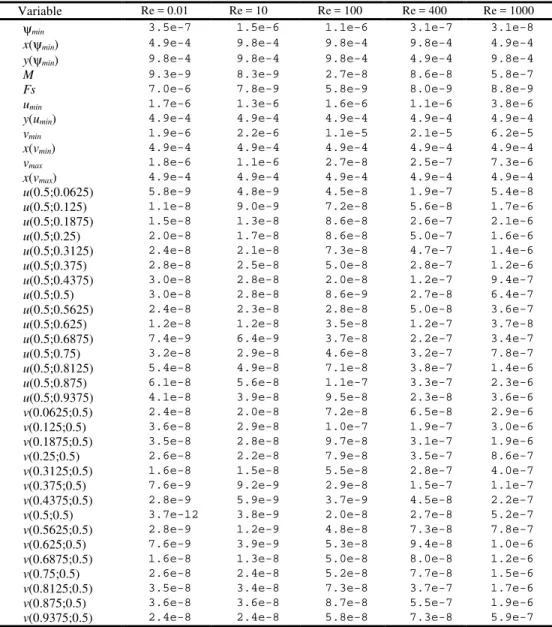
Table 7. Estimated discretization error (U) of the numerical solution (φφφφ) for the classical problem.
Variable Re = 0.01 Re = 10 Re = 100 Re = 400 Re = 1000
ψmin 3.5e-7 1.5e-6 1.1e-6 3.1e-7 3.1e-8
x(ψmin) 4.9e-4 9.8e-4 9.8e-4 9.8e-4 4.9e-4
y(ψmin) 9.8e-4 9.8e-4 9.8e-4 4.9e-4 9.8e-4
M 9.3e-9 8.3e-9 2.7e-8 8.6e-8 5.8e-7
Fs 7.0e-6 7.8e-9 5.8e-9 8.0e-9 8.8e-9
umin 1.7e-6 1.3e-6 1.6e-6 1.1e-6 3.8e-6
y(umin) 4.9e-4 4.9e-4 4.9e-4 4.9e-4 4.9e-4
vmin 1.9e-6 2.2e-6 1.1e-5 2.1e-5 6.2e-5
x(vmin) 4.9e-4 4.9e-4 4.9e-4 4.9e-4 4.9e-4
vmax 1.8e-6 1.1e-6 2.7e-8 2.5e-7 7.3e-6
x(vmax) 4.9e-4 4.9e-4 4.9e-4 4.9e-4 4.9e-4
u(0.5;0.0625) 5.8e-9 4.8e-9 4.5e-8 1.9e-7 5.4e-8
u(0.5;0.125) 1.1e-8 9.0e-9 7.2e-8 5.6e-8 1.7e-6
u(0.5;0.1875) 1.5e-8 1.3e-8 8.6e-8 2.6e-7 2.1e-6
u(0.5;0.25) 2.0e-8 1.7e-8 8.6e-8 5.0e-7 1.6e-6
u(0.5;0.3125) 2.4e-8 2.1e-8 7.3e-8 4.7e-7 1.4e-6
u(0.5;0.375) 2.8e-8 2.5e-8 5.0e-8 2.8e-7 1.2e-6
u(0.5;0.4375) 3.0e-8 2.8e-8 2.0e-8 1.2e-7 9.4e-7
u(0.5;0.5) 3.0e-8 2.8e-8 8.6e-9 2.7e-8 6.4e-7
u(0.5;0.5625) 2.4e-8 2.3e-8 2.8e-8 5.0e-8 3.6e-7
u(0.5;0.625) 1.2e-8 1.2e-8 3.5e-8 1.2e-7 3.7e-8
u(0.5;0.6875) 7.4e-9 6.4e-9 3.7e-8 2.2e-7 3.4e-7
u(0.5;0.75) 3.2e-8 2.9e-8 4.6e-8 3.2e-7 7.8e-7
u(0.5;0.8125) 5.4e-8 4.9e-8 7.1e-8 3.8e-7 1.4e-6
u(0.5;0.875) 6.1e-8 5.6e-8 1.1e-7 3.3e-7 2.3e-6
u(0.5;0.9375) 4.1e-8 3.9e-8 9.5e-8 2.3e-8 3.6e-6
v(0.0625;0.5) 2.4e-8 2.0e-8 7.2e-8 6.5e-8 2.9e-6
v(0.125;0.5) 3.6e-8 2.9e-8 1.0e-7 1.9e-7 3.0e-6
v(0.1875;0.5) 3.5e-8 2.8e-8 9.7e-8 3.1e-7 1.9e-6
v(0.25;0.5) 2.6e-8 2.2e-8 7.9e-8 3.5e-7 8.6e-7
v(0.3125;0.5) 1.6e-8 1.5e-8 5.5e-8 2.8e-7 4.0e-7
v(0.375;0.5) 7.6e-9 9.2e-9 2.9e-8 1.5e-7 1.1e-7
v(0.4375;0.5) 2.8e-9 5.9e-9 3.7e-9 4.5e-8 2.2e-7
v(0.5;0.5) 3.7e-12 3.8e-9 2.0e-8 2.7e-8 5.2e-7
v(0.5625;0.5) 2.8e-9 1.2e-9 4.8e-8 7.3e-8 7.8e-7
v(0.625;0.5) 7.6e-9 3.9e-9 5.3e-8 9.4e-8 1.0e-6
v(0.6875;0.5) 1.6e-8 1.3e-8 5.0e-8 8.0e-8 1.2e-6
v(0.75;0.5) 2.6e-8 2.4e-8 5.2e-8 7.7e-8 1.5e-6
v(0.8125;0.5) 3.5e-8 3.4e-8 7.3e-8 3.7e-7 1.7e-6
v(0.875;0.5) 3.6e-8 3.6e-8 8.7e-8 5.5e-7 1.9e-6
v(0.9375;0.5) 2.4e-8 2.4e-8 5.8e-8 7.3e-8 5.9e-7
Table 7 presents the discretization error estimated (U) through Eqs. (13) or (14) for the solution of Table 6. As can be seen, for profiles of u and v, roughly, the magnitude of U grows with Re. In the case of the remaining variables, this influence of Re on U seems to be absent. For the same Re, the magnitude of U differs considerably among several variables of interest, which can be divided into three distinct sets: (1) U is generally much lower for profiles of u and v, M and Fs; (2) vmin, vmax, umin and ψmin have a
slightly higher U; and (3) the coordinate type variables have the highest U. The magnitude of U may vary largely along the velocity profiles: the ratios between the maximum and the minimum values of U are 16,000, 47, 30, 24 and 97, respectively, for Re = 0.01, 10, 100, 400 and 1000.
Tables 8 to 13 list the results of this work and those of several other authors for the variables of interest, where Ref. indicates the works cited in Table 1. Among all results of the sixteen works reported in literature and cited here, those of Botella and Peyret (1998) are probably the most accurate. However, considering the estimated error (U) reported by Botella and Peyret (1998) and the tolerance they adopted in the iterative process, the results of the present work are probably more accurate than those of Botella and Peyret (1998). Keeping in mind that, in the present work, U is
presented in Tab. 7 and its value probably overestimates the true error; moreover, the iterative process was repeated until the achievement of machine round-off error. Among all variables of interest compared in Tables 8 to 13, the results of Botella and Peyret (1998) are probably more accurate than those of the present work only for the following variables: vmin for Re = 100 and 1000; and
vmax for Re = 1000.
It is worth noting the congruence among all results of the present work, which are compared to those of Botella and Peyret (1998). The results of Botella and Peyret (1998) lie within the interval comprised between φ±U of this work results. For example, the result of Botella and Peyret (1998) for vmax in Re = 1000 is
0.3769447, which is between 0.3769398 and 0.3769544, given in the present work. An exception is ψmin, for which Botella and Peyret
Table 8. Comparisons of ψψψψmin with other authors for the classical problem.
--- Re = 100 --- --- Re = 400 --- --- Re = 1000 --- Ref.
-ψmin x y -ψmin x y -ψmin x y
2 0.1022 0.1017
3 0.1034 0.114
4 0.1193
5 0.103423 0.6172 0.7344 0.113909 0.5547 0.6055 0.117929 0.5313 0.5625
6 0.10330 0.61667 0.74167 0.11399 0.55714 0.60714 0.11894 0.52857 0.56429
7 0.1034 0.6188 0.7375 0.1136 0.5563 0.6000 0.1173 0.5438 0.5625
9 0.103506 0.6094 0.7344 0.119004 0.5313 0.5625
10 0.1030 0.6196 0.7373 0.1121 0.5608 0.6078 0.1178 0.5333 0.5647
11 0.103519 0.6157 0.7378 0.118821 0.5308 0.5659
12 0.1157
13 0.10330 0.11389 0.118930
14 0.1189366 0.5308 0.5652
15 0.103511 0.617187 0.734375 0.118806 0.531250 0.562500
17 0.103 0.6125 0.7375 0.113 0.5500 0.6125 0.117 0.5250 0.5625
16 0.118942 0.5300 0.5650
18 0.11892 0.53125 0.56543
Present 0.1035212 0.61621 0.73730 0.11398887 0.55371 0.60547 0.118936708 0.53125 0.56543 Re = 10, Ref. 2: -ψmin = 0.0999; Present: -ψmin = 0.1001132
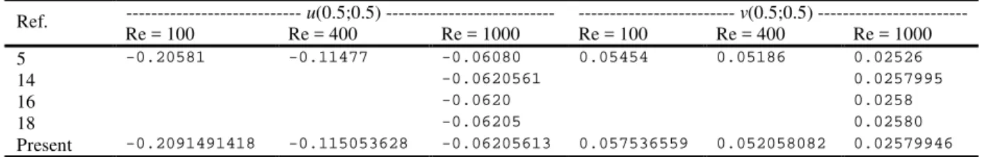
Table 9. Comparisons of u(0.5;0.5) and v(0.5;0.5) with other authors for the classical problem.
--- u(0.5;0.5) --- --- v(0.5;0.5) --- Ref.
Re = 100 Re = 400 Re = 1000 Re = 100 Re = 400 Re = 1000
5 -0.20581 -0.11477 -0.06080 0.05454 0.05186 0.02526
14 -0.0620561 0.0257995
16 -0.0620 0.0258
18 -0.06205 0.02580
Present -0.2091491418 -0.115053628 -0.06205613 0.057536559 0.052058082 0.02579946
Table 10. Comparisons of u(0.5;0.0625) and v(0.0625;0.5) with other authors for the classical problem.
--- u(0.5;0.0625) --- --- v(0.0625;0.5) --- Ref.
Re = 100 Re = 400 Re = 1000 Re = 100 Re = 400 Re = 1000
5 -0.04192 -0.09266 -0.20196 0.09233 0.18360 0.27485
14 -0.2023300 0.2807056
18 -0.20227
Present -0.041974991 -0.09259926 -0.202330048 0.094807616 0.185132290 0.2807057
Table 11. Comparisons of umin with other authors for the classical problem.
--- Re = 100 --- --- Re = 400 --- --- Re = 1000 --- Ref.
umin y umin y umin y
5 -0.21090 0.4531 -0.32726 0.2813 -0.38289 0.1719
7 -0.213 0.4578 -0.327 0.2797 -0.387 0.1734
14 -0.2140424 0.4581 -0.3885698 0.1717
Present -0.2140417 0.45850 -0.3287295 0.27979 -0.3885721 0.17139
Table 12. Comparisons of vmin with other authors for the classical problem.
--- Re = 100 --- --- Re = 400 --- --- Re = 1000 --- Ref.
vmin x vmin x vmin x
5 -0.24533 0.8047 -0.44993 0.8594 -0.51550 0.9063
14 -0.2538030 0.8104 -0.5270771 0.9092
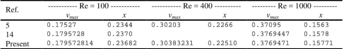
Table 13. Comparisons of vmax with other authors for the classical problem.
--- Re = 100 --- --- Re = 400 --- --- Re = 1000 --- Ref.
vmax x vmax x vmax x
5 0.17527 0.2344 0.30203 0.2266 0.37095 0.1563
14 0.1795728 0.2370 0.3769447 0.1578
Present 0.179572814 0.23682 0.30383231 0.22510 0.3769471 0.15771
Conclusion
In this work, numerical solutions were obtained for laminar flow inside a square cavity of which lid moves at variable velocity and analytical solution is known (Shih, Tan and Hwang, 1989). Results were presented for 42 variables of interest (φ) in the 1024 x 1024 nodes grid. It was found that:
1. For all variables of interest, the discretization error estimated (U) with Eqs. (13) and (14), proposed here, is reliable. In other words, U/|E| ≥ 1, where E is the true discretization error. 2. The use of multiple Richardson extrapolations (MRE) with Eq.
(12) reduced E between 1.6 x 10³ and 3.8 x 10⁶ times for velocity profiles u and v, M and Fs. This reduction was not so effective for variables vmin, vmax, umin, Fn and ψmin, which
reductions were of 1.9, 2.0, 2.6, 4.6 and 75 times, respectively. For coordinate type variables, this procedure does not apply. 3. For 34 variables, the effective order value (pE) is very close
(1.96 to 2.08) to the theoretical asymptotic order (pL) = 2
predicted a priori. For coordinate type variables, pE seems to
tend towards unity. For other variables, pE varies from 1.64 to
2.58, i.e., around pL.
The main focus of this work was to solve the problem of laminar flow inside a square cavity of which lid moves at a constant velocity and analytical solution is unknown (Kawaguti, 1961; Burggraf, 1966; Rubin and Khosla, 1977; Benjamin and Denny, 1979; Ghia, Ghia and Shin, 1982). Results were presented for 42 variables of interest (φ), and their estimated discretization errors (U) on a grid of 1024 x 1024 nodes and Reynolds numbers (Re) = 0.01, 10, 100, 400 and 1000. It was found that:
• Among all results of the sixteen works reported in literature and cited here, those of Botella and Peyret (1998) are probably the most accurate. However, considering the estimated error (U) reported by Botella and Peyret (1998) and the tolerance they adopted in the iterative process, the results of the present work are probably more accurate than those of Botella and Peyret (1998). Among all variables of interest compared in Tables 8 to 13, the results of Botella and Peyret (1998) are probably more accurate than those of the present work only for the following variables: vmin for Re = 100 and 1000; and vmax for Re = 1000.
There is a notable consistency among all results of the present work, comparing them with those of Botella and Peyret (1998): the results of Botella and Peyret (1998) fall inside the interval comprised between φ±U of the results of the present work.
• For velocity profiles u and v, the apparent order (pU) varies from
1.76 to 2.34, with most of the results very close to the theoretical value of pL = 2 which was predicted a priori. For
coordinate type variables, pU seems to tend towards unity. In
only five cases out of more than 200, the value of pU varied
from 1.10 to 1.63, remaining distant from pL. An exception is
the variable Fn: its value does not converge with the grid refinement, causing pU to tend towards zero. This is apparently
due to the discontinuity in the boundary condition (B.C.) of u at lid corners. For Fs, which does not present discontinuities in the B.C., the solution converges with the grid refinement, with pU
varying from 1.33 to 2.03 for the five values of Re.
Acknowledgments
The second author gratefully acknowledges the support provided by the Laboratory of Numerical Experimentation (LENA), at Federal University of Paraná (UFPR), and the guidance of Professors Carlos Henrique Marchi and Fábio Alencar Schneider, as well as CAPES (Coordenação de Aperfeiçoamento de Pessoal de Nível Superior) – Brazil for granting a scholarship. And the first author thanks the support of CNPq (Conselho Nacional de Desenvolvimento Científico e Tecnológico) – Brazil for granting him a scholarship. The authors acknowledge The “UNIESPAÇO Program” of The Brazilian Space Agency (AEB) and thank the two referees for their suggestions and comments.
References
Barragy, E. and Carey, G.F., 1997, “Stream function-vorticity driven cavity solution using p finite elements”, Computers & Fluids, Vol. 26, pp. 453-468.
Benjamin, A.S. and Denny, V.E., 1979, “On the convergence of numerical solutions for 2-D dlows in a cavity at large Re”, Journal of Computational Physics, Vol. 33, pp. 340-358.
Botella, O. and Peyret, R., 1998, “Benchmark spectral results on the lid-driven cavity flow”, Computers & Fluids, Vol. 27, pp. 421-433.
Bruneau, C.H. and Saad, M., 2006, “The 2D lid-driven cavity problem revisited”, Computers & Fluids, Vol. 35, pp. 326-348.
Burggraf, O.R., 1966, “Analytical and numerical studies of the structure of steady separated flows”, Journal of Fluid Mechanics, Vol. 24, pp. 113-151.
De Vahl Davis, G., 1983, “Natural convection of air in a square cavity: a bench mark numerical solution”, International Journal for Numerical Methods in Fluids, Vol. 3, pp. 249-264.
Erturk, E., Corke, T.C. and Gökçöl, C, 2005, “Numerical solutions of 2D steady incompressible driven cavity flow at high Reynolds numbers”,
International Journal for Numerical Methods in Fluids, Vol. 48, pp. 747-774. Ferziger, J.H. and Peric, M., 1999, “Computational Methods for Fluid Dynamics”, Springer-Verlag, Berlin, Germany, 2 ed., 389 p.
Ghia, U., Ghia, K.N. and Shin, C.T., 1982, “High-Re solutions for incompressible flow using the Navier-Stokes equations and a multigrid method”, Journal of Computational Physics, Vol. 48, pp. 387-411.
Goyon, O., 1996, “High-Reynolds number solutions of Navier-Stokes equations using incremental unknowns”, Computer Methods in Applied Mechanics and Engineering, Vol. 130, pp. 319-335.
Gupta, M.M. and Kalita, J.C., 2005, “A new paradigm for solving Navier-Stokes equations: streamfunction-velocity formulation”, Journal of Computational Physics, Vol. 207, pp. 52-68.
Hayase, T., Humphrey, J.A. and Greif, R., 1992, “A consistently formulated QUICK scheme for fast and stable convergence using finite-volume iterative calculation procedures”, Journal of Computational Physics, Vol. 98, pp. 108-118.
Hou, S., Zou, Q., Chen, S., Doolen, G. and Cogley, A.C., 1995, “Simulation of cavity flow by lattice Boltzmann method”, Journal of Computational Physics, Vol.118, pp. 329-347.
Kawaguti, M., 1961, “Numerical solution of the Navier-Stokes equations for the flow in a two-dimensional cavity”, Journal of the Physical Society of Japan, Vol. 16, pp. 2307-2315.
Khosla, P.K. and Rubin, S.G., 1974, “A diagonally dominant second-order accurate implicit scheme”, Computers & Fluids, Vol. 2, pp. 207-209.
Kreyszig, E., 1999, “Advanced Engineering Mathematics”, Wiley, New York, United States of America, 8 ed., 1156 p.
Marchi, C.H. and Maliska, C.R., 1994, “A nonorthogonal finite-volume method for the solution of all speed flows using co-located variables”,
Numerical Heat transfer, Part B, Vol.26, pp. 293-311.
Marchi, C. H. and Silva, A.F.C., 2002, “Unidimensional numerical solution error estimation for convergent apparent order”, Numerical Heat Transfer, Part B, Vol. 42, pp. 167-188.
Nie, X., Robbins, M.O. and Chen, S., 2006, “Resolving singular forces in cavity flow: multiscale modeling from atomic to millimeter scales”,
Physical Review Letters, Vol.96 (134501), pp. 1-4.
Nishida, H. and Satofuka, N., 1992, “Higher-order solutions of square driven cavity flow using a variable-order multi-grid method”, International Journal for Numerical Methods in Engineering, Vol. 34, pp. 637-653.
Richardson, L. F., 1910, “The approximate arithmetical solution by finite differences of physical problems involving differential equations, with an application to the stresses in a masonry dam”, Phylosophical Proceedings of the Royal Society of London Serial A, Vol. 210, pp. 307-357.
Roache, P.J., 1994, “Perspective: a method for uniform reporting of grid refinement studies”, ASME Journal of Fluids Engineering, Vol. 116, pp. 405-413.
Roache, P.J., 1998, “Verification and Validation in Computational Science and Engineering”, Hermosa, Albuquerque, United States of America, 446 p.
Rubin, S.G. and Khosla, P.K., 1977, “Polynomial interpolation methods for viscous flow calculations”, Journal of Computational Physics, Vol. 24, pp. 217-244.
Schneider, F.A., 2007, “Verification of Numerical Solutions in Diffusive and Advective Problems with Nonuniform Grids” (in Portuguese), Ph.D. thesis, Federal University of Paraná, Curitiba, Brazil, 223 p.
Schneider, G.E. and Zedan, M., 1981, “A modified strongly implicit procedure for the numerical solution of field problems”, Numerical Heat Transfer, Vol. 4, pp. 1-19.
Schreiber, R. and Keller, H.B., 1983, “Driven cavity flows by efficient numerical techniques”, Journal of Computational Physics, Vol. 49, pp. 310-333.
Shih, T.M., Tan, C.H. and Hwang, B.C., 1989, “Effects of grid staggering on numerical schemes”, International Journal for Numerical Methods in Fluids, Vol. 9, pp. 193-212.
Van Doormaal, J.P. and Raithby, G.D., 1984, “Enhancements of the SIMPLE method for predicting incompressible fluid flow”, Numerical Heat Transfer, Vol. 7, pp. 147-163.
Vanka, S.P., 1986, “Block-implicit multigrid solution of Navier-Stokes equations in primitive variables”, Journal of Computational Physics, Vol. 65, pp. 138-158.
Wright, N.G. and Gaskell, P.H., 1995, “An efficient multigrid approach to solving highly recirculating flows”, Computers & Fluids, Vol. 24, pp. 63-79.