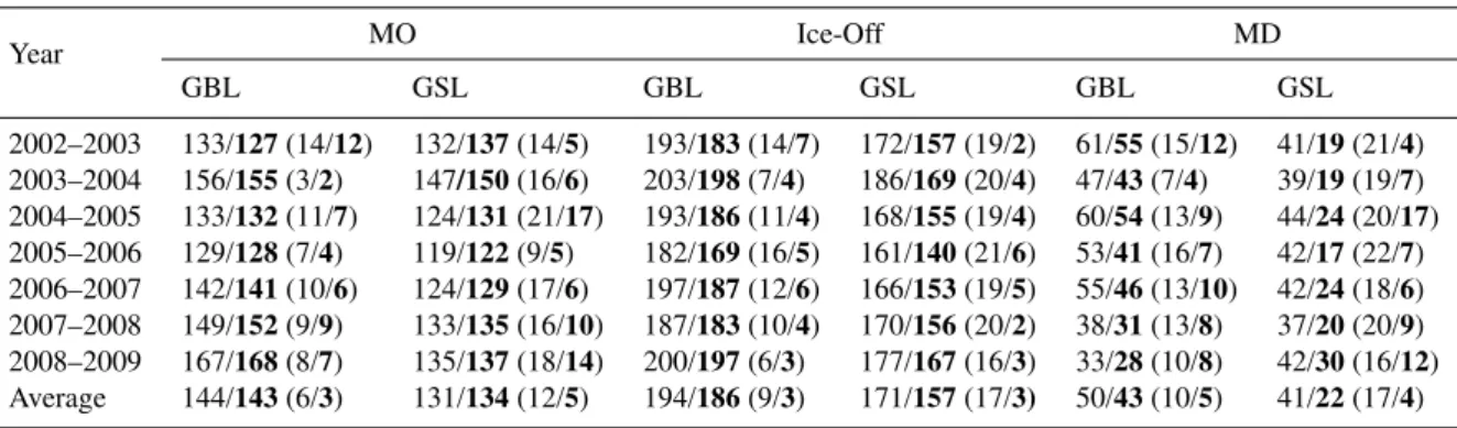
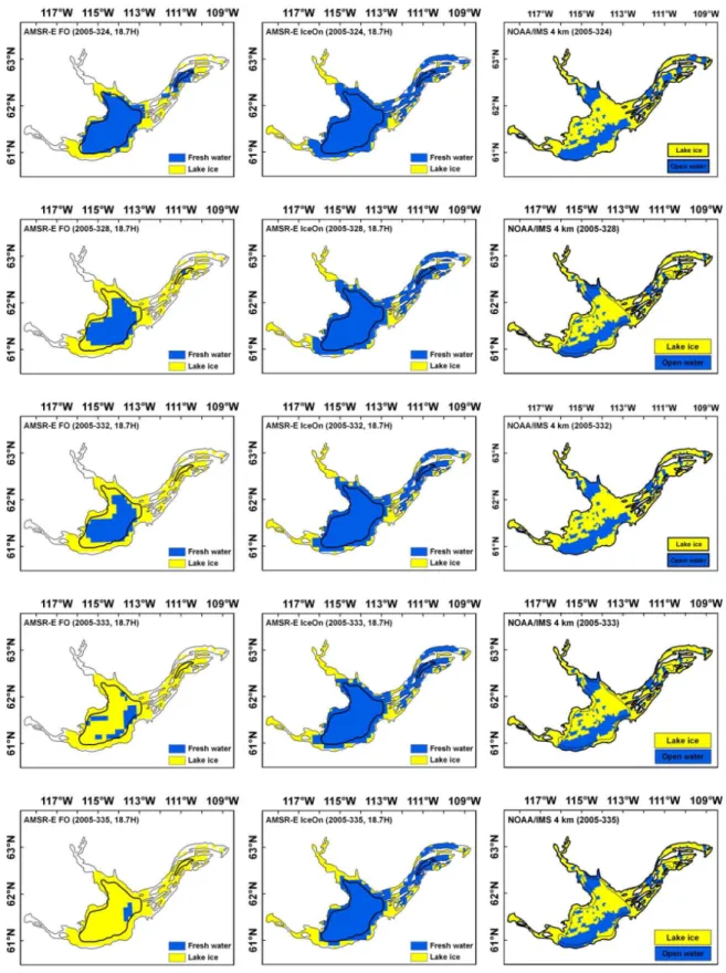
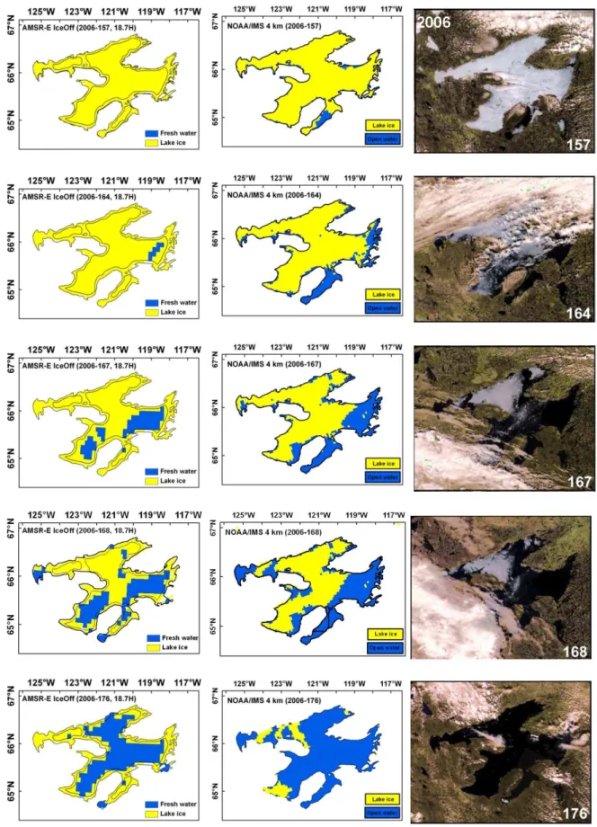
Estimating ice phenology on large northern lakes from AMSR-E: algorithm development and application to Great Bear Lake and Great Slave Lake, Canada

The probability of attending school four our group of interest in this region increased by 6.5 percentage points after the expansion of the Bolsa Família program in 2007 and

The activities carried out by the Institute of Nutrition of Central America and Panama (INCAP) directed toward the development of a vegetable mixture known by the generic

De esta forma cuando un sujeto mira un objeto desde el lugar del deseo, el objeto le está devolviendo la mirada, pero desde un lugar en que el sujeto no puede verlo, escisión entre

Utilizan variados ornamentos, ilustraciones y tipografía según la disponibilidad de las imprentas que, de a poco, van mejorando sus talleres e implementos: la del diario

This dissertation will first describe the AGM Model and the modified postulates of AGM, as defined by Katsuno and Mendelzon [KM91]. Some revision models will be characterized.

In the State of Ceará (Northeast Brazil), scom- brid abundance is greater from October to March (transition from wet to dry season) (Fonteles-Fi- lho, 1968; Costa & Paiva,

O cruzamento dos dados apresentados nos dois relatórios cumpre o primeiro sub objetivo deste trabalho. Uma analise geral desses resultados nos permite compreender o