SRef-ID: 1607-7946/npg/2005-12-849 European Geosciences Union
© 2005 Author(s). This work is licensed under a Creative Commons License.
Nonlinear Processes
in Geophysics
On the predictability of ice avalanches
A. Pralong1, C. Birrer2, W. A. Stahel2, and M. Funk1
1Laboratory of Hydraulics, Hydrology and Glaciology, Swiss Federal Institute of Technology, 8092 Z¨urich, Switzerland 2Seminar for Statistics, Swiss Federal Institute of Technology, 8092 Z¨urich, Switzerland
Received: 13 June 2005 – Revised: 19 August 2005 – Accepted: 19 August 2005 – Published: 30 September 2005
Abstract. The velocity of unstable large ice masses from hanging glaciers increases as a power-law function of time prior to failure. This characteristic acceleration presents a finite-time singularity at the theoretical time of failure and can be used to forecast the time of glacier collapse. How-ever, the non-linearity of the power-law function makes the prediction difficult. The effects of the non-linearity on the predictability of a failure are analyzed using a non-linear re-gression method. Predictability strongly depends on the time window when the measurements are performed.
Log-periodic oscillations have been observed to be super-imposed on the motion of large unstable ice masses. The value of their amplitude, frequency and phase are observed to be spatially homogeneous over the whole unstable ice mass. Inclusion of a respective term in the function describing the acceleration of unstable ice masses greatly increases the ac-curacy of the prediction.
1 Introduction
The prediction of ice avalanches from hanging glaciers is based on the progressive acceleration observed on large un-stable ice masses prior to their collapse. A suitable model of the observed acceleration presents a finite time singularity; that is, the velocity tends to infinity as the time approaches a finite time. This finite time corresponds to the time of failure. Finite time singularity models have been used for char-acterizing a large variety of phenomena. Rheologists have suggested such models to describe the ductile fracture of samples of rock, soil, high-performance metal alloys, con-crete, polymers and ice (see Varnes, 1983 for a review and Voitkovskii, 1960; Szyszkowski and Glockner 1986; Mahrenholtz and Wu 1992 for laboratory ice). At large scales, finite time singularity models have been proposed to describe the mechanisms of landslides (e.g. Crosta and Correspondence to:M. Funk
Agliardi, 2003; Amitrano et al., 2005), earthquakes1 (e.g. Bufe and Varnes, 1993; Bowman et al., 1998), volcanic eruptions (e.g. Voight, 1988), fracture of structures (e.g. Jo-hansen and Sornette, 2000), inflation (Sornette et al., 2003), finance, economy, population (Johansen and Sornette, 2001) and break-off of ice chunks from hanging glaciers (Haeberli, 1975; Flotron, 1977; Iken, 1977; R¨othlisberger, 1981; L¨uthi, 2003; Pralong and Funk, 2005a,b).
Finite-time singularities are caused by positive feedback processes, which lead to a catastrophic evolution of the ob-served quantities. Sammis and Sornette (2002) reviewed pos-itive feedbacks involved in the rupture of materials; Sornette et al. (2003) mentioned a positive feedback involved in infla-tion.
A suitable model for such catastrophic evolutions is given by Voight’s differential equation (Voight, 1988)
¨
f =A f˙α, (1)
where the dot denotes the time derivative and f (t;A, α, c1, c2)is the function describing the temporal evolution of
a measured quantity. ObservationsYi are obtained at times ti. They include a random disturbanceZi, i.e.
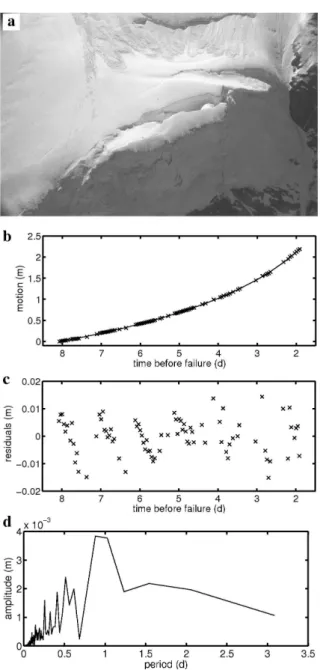
Fig. 1. Data set of Gruben glacier, Switzerland. (a)Photo of a calving event similar to the one measured by Haeberli (1975). The unstable mass is visible in the foreground. (b) Measured relative velocityY˙ (Haeberli, 1975) versus time (crosses) and its associ-ated fit (solid line) based on Eq. (6). The estimassoci-ated parametersθˆi
of Eq. (6) are listed in Table 1. The predicted failure time (corre-sponding to abscissa zero) was 9 September 1974.(c)Residuals of the fit. The solid line indicates the fit of the log-periodic oscillations (see Sect. 5).
Integrating Eq. (1) forα>1 and assuming thatf˙at the time of the singularity is infinite, leads to (Voight, 1988)
f (t,θ)= θ
4−θ3ln(θ1−t ) if θ2=0 θ4−θθ3
2 (θ1−t )
θ2 if θ
26=0 , (3)
withθ1the time of failure,θ4a constant and θ2=
α−2
α−1 <1 and θ3=(A (α−1))
θ2−1. (4)
For the failure of hanging glaciers, observations and numer-ical simulations (Haeberli, 1975; Iken, 1977; Pralong and Funk, 2005a) show that the relative motion of an unstable ice mass (relative to the motion of the stable glacier part lo-cated directly upstream of the unstable part) is adequately
described by Eq. (1); that is, the relative motion of the unsta-ble ice masses can be modeled byf 2.
Two different approaches can be applied in order to pre-dict the time of failureθ1: a “rheological” and an
“empiri-cal” approach. The rheological approach considers Eq. (1) (or a similar equation) as a constitutive relation for the evo-lution ofY and looks for general relations for the parameters A=A(σ, T , ...)andα=α(σ, T , ...), which may depend, for example, on the stressσ and the temperatureT. An a priori knowledge of A andα (or equivalently of θ2 andθ3)
per-mits then to estimate the time of failureθ1. For example, by
settingA=B(T ) σr,α=k+2 andY˙=1/(1−D), whereB(T ) is a function of temperature, r andk are material parame-ters andDis the classical damage variable of the continuum damage mechanics (e.g. Lemaitre, 1996), Voight’s equation (Eq. 1) reduces to
˙
D=B(T ) σr(1−D)−k. (5)
This equation is the classical Kachanov-Rabotnov constitu-tive relation (Kachanov, 1957; Rabotnov, 1969), modeling the accumulation of isotropic damage in material subject to uniaxial load. Equation (5) describes, therefore, a finite time singularity ifk>−1 (i.e. α>1). The rheological approach is appropriate for describing the fracture of homogeneous samples of ductile materials; however, a precise prediction cannot be obtained. The application of this method to the description of the failure of large-scale structures by the in-tegration of a local damage evolution law (e.g. Eq. 5) in a large-scale domain can lead to an adequate capture of the physics of the global fracture (e.g. Lyakhovsky et al. (2001) for earthquakes, and Pralong and Funk (2005a) for fracture processes in glaciers), but fails to predict accurately the time of the global failure, since the conditions prevailing before the failure process are largely unknown and the parameters are subject to uncertainties.
In the empirical approach, in contrast to the rheological approach,Aandα(orθ2andθ3, respectively) are not a
pri-ori determined. The prediction of the failure timeθ1is thus
a fitting problem of measured data, where the critical quan-tityY is compared to the solution of Voight’s equation, and the parameters of Eq. (3) and especially θ1 are estimated.
This approach turns out to be more precise than the rheolog-ical approach, since the a priori informations needed for the rheological approach are affected by uncertainties. This ap-proach is usually applied to the prediction of the singularity of large-scale processes, which can cause great damage. In such a case, precise prediction allows for preventive actions. This paper focuses on the empirical approach applied to the destabilization of ice chunks from hanging glaciers.
2 Measurements
The motion of several unstable ice masses was monitored by the Laboratory of Hydraulics, Hydrology and Glaciology (VAW) of the Swiss Federal Institute of Technology Z¨urich (ETHZ) within the scope of hazard assessment or research programmes. Of the various data sets collected, three will be considered here. The others do not contain enough measure-ments or are affected by a scattering that is too broad to be useful.
The first data set describes the relative motion of a calv-ing ice mass (Figs. 1a and b) measured by Haeberli (1975) at Gruben glacier, Switzerland. The measurement equipment was a wire fixed at one end to the unstable ice mass and at the other end to a dial gauge attached to the stable part of the glacier. The time of failure was registered. Haeberli con-sidered the relative velocityY˙ (time derivative of the motion Y) of the unstable ice mass instead of the relative motionY. The function used to describeY˙is thus the time derivative of Eq. (3):
˙
f (t,θ)=θ3(θ1−t )θ2−1. (6)
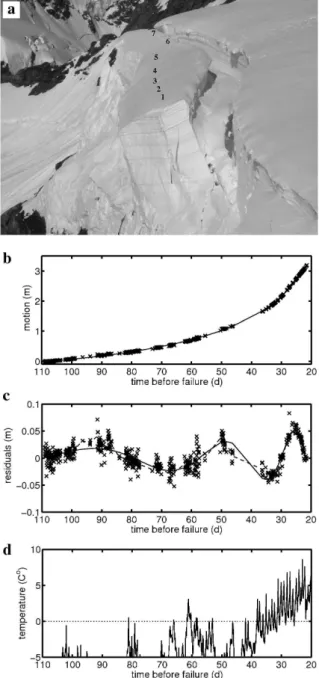
The second data set corresponds to the acceleration of an unstable ice mass measured by the authors in 2001 at the front of the Eiger hanging glacier, Switzerland (Figs. 2a and b). The measurement equipment was a theodolite laser-distometer installed at Eiger glacier (a fixed position near the glacier) and one reflector mounted on a stake drilled into the unstable ice mass. Reference reflectors installed on a rock face close to the unstable ice mass enabled the correction of the measurements, which are influenced by meteorological conditions. For this data set, only the absolute motion (de-noted byYa) is known. The motion of the stable glacier part upstream of the unstable ice mass was not measured. It is assumed that during the measurements, the velocity of the stable glacier part is constant. The function which models the motionYareads
fa(t,θ)= θ
5t+θ4−θ3ln(θ1−t ) if θ2=0 θ5t+θ4−θθ3
2(θ1−t )
θ2 if θ
26=0 , (7)
withθ5 the constant velocity of the upstream glacier part.
The time of failure of the unstable mass is not known as a subfailure occurred prior to the main failure, and caused the measurement equipment on the glacier to be lost.
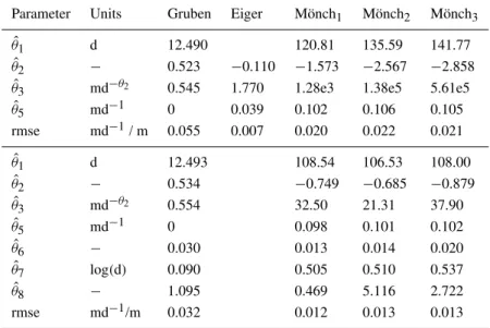
The third data set describes the motion of several material points (stakes with reflectors) installed on a single unstable ice mass at the front of the M¨onch hanging glacier, Switzer-land (Fig. 3a). The measurements were performed by the authors in 2003, with the same equipment as for the Eiger hanging glacier. The three material points used for the anal-ysis correspond to points 1, 2 and 3 of Fig. 3a. Points 4 and 5 present a temporal shift of the beginning of the acceleration (relatively to points 1, 2 and 3) and points 6 and 7 showed no acceleration during the period of measurement. The mo-tion of point 1 is shown in Fig. 3b as an example. The time of failure of the unstable ice mass is unknown, for the same
rea-Fig. 2. Data set of Eiger glacier, Switzerland. (a)Photo of the measured unstable ice mass. The unstable mass is approximately 60 m high, 150 m long (direction normal to the ice flow) and 30 m wide. (b)MotionYa−θ5tversus time (crosses) and its associated fit (solid line) based on Eq. (7). The estimated parametersθˆi of
Eq. 7 are listed in Table 1. The predicted failure time (correspond-ing to abscissa zero) was 20 August 2001. (c)Residuals of the fit.
d)Fourier analysis of the residuals.
son as for the Eiger measurements3. The measurements were affected by slight variations in the position of the theodolite
Fig. 3. Data set of M¨onch glacier, Switzerland. (a)Photo of the measured unstable ice mass. The numbers indicate the location of the measured points. The unstable mass is approximately 50 m high, 300 m long (direction normal to the ice flow) and 40 m wide. The distance between points 1, 2 and 3 amounts to approximately 30 m. (b)MotionYa−θ5tversus time (crosses) of point 1 and its associated fit (solid line) based on Eq. (7). The estimated parame-tersθˆi of Eq. (7) are listed in Table 1. The predicted failure time
(corresponding to abscissa zero) was July 4, 2003.(c)Residuals of the fit. The solid line indicates the fit of the log-periodic oscillations (see Sect. 5). The dashed line shows the smooth cruve of the residu-als.(d)Air temperature at Jungfraujoch (MeteoSwiss data) located one kilometer from the glacier (solid line). The dotted line depicts the ice melting point.
(Appendix A). To account for these variations, the position of the theodolite was calculated at each measurement cycle
from the position of four reference reflectors located on rock faces around the theodolite (Appendix A). Again, only the absolute motionYais known. It is modeled by Eq. (7). It will again be assumed that the velocity of the stable glacier part is constant. For this data set, this assumption is questionable, since a significant increase in the air temperature above the melting point occurred during the failure process (Fig. 3d), and could have caused an acceleration of the glacier, thereby modifying the velocity θ5. The measurements revealed a
variation in the velocityY˙aof points 4 and 5 which could be related either to air temperature4or to the beginning of the destabilization process. For points 1, 2 and 3, the measure-ments did not reveal variations in the velocity which could be related to air temperature.
The estimates of the parametersθi (using a least squares method) for the failure of the three different glaciers are re-ported in Table 1. The residuals from the fits are shown in Figs. 1c, 2c and 3c. For the Gruben data set, the estimated failure timeθ1 occurred some minutes before the observed
failure. The residuals of the Eiger data set show strong os-cillations. The Fourier analysis (Fig. 2d) revealed a domi-nant frequency corresponding to one day. Since the absolute motionYais considered, these oscillations can be associated to the daily fluctuations of the basal sliding. Such fluctua-tions are commonly observed on glaciers (e.g. Sugiyama and Gudmundsson, 2003). The residuals of the M¨onch data set show clear log-periodic oscillations. This behavior will be discussed in Sect. 5. Because of the few data points, the residuals of the Gruben data set do not allow to validate the presence of log-periodic oscillations. Nevertheless, the data set has been tentatively fitted by using the model with log-periodic oscillations5.
3 Non-linear regression analysis
The aim of this section is to present a method to obtain es-timates of the parameters of the non-linear function 3 and their confidence intervals. The data set of the Gruben glacier is considered for illustration (Fig. 1).
The fitting process should account for the fact that the fail-ure time must be greater than the time of the last observation;
4The following model is considered to support the analysis of the dependence of the glacier velocity to the air temperature. A lin-ear water reservoir model (e.g. Hock and Noetzli, 1997) is used to estimate the water level in the glacier. The water supply of the reser-voir is the water resulting from the melt of the snow covering the glacier. The melting rate is estimated with the air temperature. The water level can then be related to the basal sliding and the glacier velocity (e.g. Sugiyama and Gudmundsson, 2003).
Table 1.Values of the estimated parametersθˆi for the five data sets analyzed in this paper. The values ofθˆ2toθˆ5in the upper part of the table are identified by using the model without log-periodic oscillations (Eq. 6 or 7). The values ofθˆ1toθˆ8in the lower part of the table are identified by using the model with log-periodic oscillations (Eq. 12 or 13, see Sect. 5).θ1andθ4are integration constants. They depend on the value oft0andY (t0), and do not influence the shape of the acceleration (the differential Eq. (1) depends only onαandA; that is not onθ1andθ4). They are thus not reported in this table. Only the values ofθˆ1corresponding to the measurements at Gruben and M¨onch are reported for discussion (see text). The value of the estimated parameter of the steady motion (θˆ5) vanishes for the measurement at Gruben, since the relative motion of the unstable ice mass was measured. The values of the parameters corresponding to the model with log-periodic oscillations have not been determined for the measurements at Eiger, since no oscillations were observed (see text). The root-mean-square error (rmse) is also reported for the fits with and without log-periodic oscillations. The unit md−1refers to the Gruben data set (velocity of the unstable ice mass) and the unit m to the other data sets (displacement of unstable ice masses).
Parameter Units Gruben Eiger M¨onch1 M¨onch2 M¨onch3
ˆ
θ1 d 12.490 120.81 135.59 141.77
ˆ
θ2 − 0.523 −0.110 −1.573 −2.567 −2.858 ˆ
θ3 md−θ2 0.545 1.770 1.28e3 1.38e5 5.61e5 ˆ
θ5 md−1 0 0.039 0.102 0.106 0.105
rmse md−1/ m 0.055 0.007 0.020 0.022 0.021
ˆ
θ1 d 12.493 108.54 106.53 108.00
ˆ
θ2 − 0.534 −0.749 −0.685 −0.879
ˆ
θ3 md−θ2 0.554 32.50 21.31 37.90
ˆ
θ5 md−1 0 0.098 0.101 0.102
ˆ
θ6 − 0.030 0.013 0.014 0.020
ˆ
θ7 log(d) 0.090 0.505 0.510 0.537
ˆ
θ8 − 1.095 0.469 5.116 2.722
rmse md−1/m 0.032 0.012 0.013 0.013
that is,θ1>max(ti). Moreover, according to Eq. 4, θ2<1.
The following parameter transformations force the parame-tersθito satisfy these constraints:
θ1=max(ti)+exp(φ1), θ2=1−exp(φ2), θ3=φ3,(8)
whereφis the new parameter set off˙.
The subplots on the diagonal of the Fig. 4 are the profile-t plots, the other subplots are the profile traces. The profile-t plots show the dependence of the profile-tfunctionτkon the parametersφk(solid line).τkis the signed square root of the likelihood ratio test statistic for a null hypotheses aboutφk (Appendix B; Bates and Watts, 1988). In comparison, the test statistic based on the linear approximation of the regres-sion inφˆ (the estimateφˆ is depicted by a cross) is displayed using a dash-dotted line. It is linear inφk. The confidence interval derived fromτ (Appendix B) is depicted by dashed lines, and the confidence interval derived from the linearized statistic test by dotted lines. Since the linear approximations are excellent, the difference can barely be seen.
The off-diagonal diagrams display the profile traces (Ap-pendix B; Bates and Watts, 1988). They represent the corre-lations between the different parametersφiin the vicinity of
ˆ
φ. In each profile subplot, the closer the two lines are to each other, the more the parameters of the subplot are correlated.
4 Sensitivity analysis
This section attempts to determine the influence of the mea-surement scheme on the accuracy of the prediction. The ac-curacy of the prediction is quantified by the size of the confi-dence interval for the time of failure.
4.1 Method
The set of the measurement times(t1, ..., tn)and the accu-racy of the measurements are fixed by the parameter setS S=(σY, δY, 1tE, 1tB) , (9)
whereσY is the standard deviation of the measurements,δY is the periodicity of the measurements, 1tE=θ1−tE is the
time span between the end of the measurements (at timetE)
and the failure (at timeθ1) and1tB=θ1−tBis the time span
between the beginning of the measurements (at timetB) and
the failure.
In order to analyze the sensitivity of the accuracy of the prediction to the parametersSi, a collection of synthetic data sets is created with Eq. (3) by using the values of the parame-tersθiidentified for three analyzed break-off events (Gruben, Eiger, M¨onch1; Table 1) and with different sets of
Fig. 4.Non-linear regression analysis of the Gruben data set (see text). The diagonal diagrams show the profile-tplots. The 95% confidence interval of each parameter is indicated by dashed lines. The off-diagonal diagrams show the profile traces. The 95% confidence contours (dotted lines) of the pair-parameters are also shown.
The periodicity of the measurements is supposed to be con-stant with time and to equalδY. In this section, we assume no further disturbances (like daily variations of θ5 or
log-periodic oscillations), even though they could influence the accuracy of the forecast. The disturbanceZ has, therefore, a constant centered normal distribution and no time correla-tion.
The sensitivity analysis consists in letting the parameters Si vary independently around defined reference valuesS∗ i and analyzing the effect of these variations on the confidence interval ofθ1by using the non-linear regression analysis
pre-sented in Sect. 3. The reference valuesS∗
i are set at S∗= σY∗=0.01 m, δY∗=0.05 d, 1tE∗=3 d, 1tB∗=30 d
. (10) The value σY∗ is given by the accuracy of today’s theodo-lite laser-distometers6.δ∗Y corresponds approximately to one measurement per hour. Experience has shown that a precise prediction emerges only a few days before the effective col-lapse. Therefore, 1tE∗ is chosen as three days. 1tB∗ corre-sponds to a time series of measurements (until failure) of one
6This accuracy is obtained by normalizing each measurement with reference measurements (in a similar way to the method used for differential GPS measurements).
month. The unstable ice chunks are regularly losing mass by fracture during the acceleration process. If the detached mass is significant, the acceleration of the remaining unsta-ble ice part shows a discontinuity. In that case, the data are not described by Eq. (1) anymore. Other phenomena, like ice melting or strong variations in basal sliding may also affect the acceleration of the unstable ice mass (Pralong and Funk, 2005b). The time span1tBused for a prediction should
cor-respond to the last time span prior to the failure during which no external disturbances interfere with the failure process. The reference value1tB∗corresponds to a mean of values ob-served in practice.
For this analysis, it will be assumed that the relative mo-tionY of the unstable ice mass is known. Therefore, Eq. (3) (with parameters θ1 to θ4) is considered. The parameter
transformation as given by Eq. (8) is applied to the four pa-rametersθi
θ1=max(ti)+exp(φ1), θ2=1−exp(φ2),
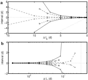
Fig. 5. Influence of the value of1tE(a)and1tB(b)on the 95% confidence interval ofθ1. The solid lines with the marks ”×” (the dashed lines with ”◦” and the dash-dotted lines with ”+”, respec-tively) are calculated by analyzing data sets synthesized with Eq. 3 and the valuesθˆi (see Table 1) estimated from the measurements
at Gruben (Eiger and M¨onch1, respectively). The horizontal dotted lines on both panels correspond to the estimate ofθ1. The inclined dotted line in panel a) and the vertical dotted line in panel b) depict the timetEof the end of the measurements.
4.2 Results and discussion
The variations in the 95% confidence interval for θ1 as a
function of Si are presented in Fig. 5. For the three ana-lyzed break-off events (Gruben, Eiger, M¨onch1), the results
are qualitatively similar. The influence ofσY andδY is here similar to the case of a linear regression and is not presented (the size of the confidence interval is proportional toσY and toδY0.5). Only the influence of1tEand1tBis considered.
The size of the confidence interval decreases with decreasing 1tE (Fig. 5a), since the information about the failure time
contained in the data sets becomes more accurate astEtends
to θ1. The size of the confidence interval decreases with
increasing1tB (Fig. 5b), since a longer time span of
mea-surements reduces the effects of the inaccuracy of individual measurements.
The analysis of the profile-t plots shows that thet-profile τ (φ1)remains approximately linear for all1tEand1tB(for
the influence of1tE onτ (φ1)see Fig. 6). The confidence
interval ofφ1is therefore symmetric. The asymmetry of the
confidence interval forθ1observed in Fig. 5 is due to the
non-linearity of the parameter transformation 111. The analysis of
the profile traces shows that1tEand1tBstrongly influence
the correlation between θ1 andθi6=1 (for 1tE, see Fig. 6).
The correlation between the parameters strongly influences the size of the confidence interval.
Figure 5a shows that accurate long-term predictions are difficult. The confidence interval ofθ1is small only if the
time span between tE and the time of failure does not
ex-ceed a few days. For earlier end pointstE, the confidence
interval is large and its lower boundary tends toward the line corresponding to the timetEof the last measurement (the
in-clined dotted line in Fig. 5a). This suggests that a forecast performed at an early stage of the destabilization can falsely lead to the prediction of an impending failure. This problem was observed by Bufe and Varnes (1993) for the prediction of earthquakes and experienced by the authors during the pre-diction of the failure of hanging glaciers. To estimate the quality of the prediction of an impending failure, the uncer-tainty on the forecast has to be determined or/and an a priori value of the parameters θ2 andθ3 has to be approximately
known.
For practical application, σY is constrained by the mea-surement method,1tEis continuously decreasing during an
ongoing measurement process andδY, and1tBare free
pa-rameters. To improve the accuracy of the prediction,σY can be decreased by considering the mean of repeated measure-ments orδY simply decreased. However, the measurements at Eiger and M¨onch (Figs. 2c and 3c), revealed that the dis-turbance Z is a correlated noise for time lags of less than one day7. For such a noise, measurements with a lag less than one day do not improve the accuracy of the prediction. During a destabilization process, it is attempted to conduct measurements until failure occurs, in order to continuously improve the prediction. However, for technical reasons, the measurements could be interrupted prior to the failure. If 1tEis too large, the prediction is inaccurate. 1tBis chosen
as large as possible, but is limited by the presence of external disturbances which may impose the value oftB(see above).
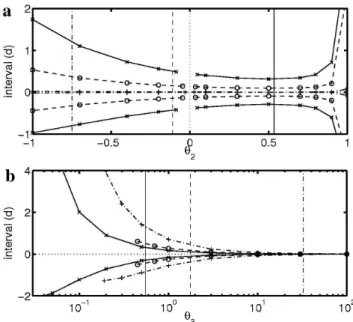
The differences in the size of the confidence intervals ob-served in Fig. 5 for the destabilization processes at Gruben, Eiger and M¨onch are due to different values of the param-etersθ2andθ3(Table 1). Figure 7a shows the influence of
the variation inθ2 on the confidence interval ofθ1, the
pa-rameterθ3and the parameter setSremaining constant. The
minimum of the confidence interval corresponds to approxi-matelyθ2=0.6. Figure 7b shows the influence of the
varia-tion inθ3on the confidence interval ofθ1, the parameterθ2
and the parameter setS remaining constant. A large value ofθ3is associated with an important displacement of the
un-stable ice mass during the failure process; that is, the noise Z becomes small relative to the variations inY (the size of the confidence interval is proportional to θ3−1). Therefore,
Fig. 6.Influence of1tEon the profilet-plots and profile traces. The non-linear regression analysis is based on two data sets synthesized with Eq. (3) and the value of the Eiger parametersθilisted in Table 1. The value of the parametersSiis for a)S= σY∗, fY∗, 1tE=0.1 d, 1tB∗
larger values of θ3 decrease the confidence interval of θ1.
This effect explains the main differences in the size of the confidence interval observed between the different break-off events in Fig. 5.
5 Log-periodic oscillations
5.1 Background
Log-periodic oscillations are characteristic oscillations which may occur during a critical process leading to a finite-time singularity. They are superimposed on the motionf (t ) with a frequency proportional to log(θ1−t ). They appear as
solutions of Voight’s equation when the exponentθ2becomes
complex (Sornette and Sammis, 1995). Forθ26=0, the real
partflpo(t,θ)of the model function with oscillations takes
the form (Sornette and Sammis, 1995) flpo(t,θ)=θ4−θθ32 (θ1−t )θ2 ·
h
1+θ6sin
2πlog(θ1−t )
log(θ7) +θ8
i
, (12)
whereθ6is the relative amplitude8,θ7is the logarithmic
pe-riodicity andθ8is the phase shift of the log-periodic
oscil-lation. An acceleration with oscillations, which is superim-posed on a steady motion takes the form
flpoa (t,θ)=θ5t+θ4−θθ32(θ1−t )θ2 · h
1+θ6sin
2πlog(θ1−t )
log(θ7) +θ8
i
. (13)
Log-periodic oscillations have been observed for numerous finite-time singularities: fracture of structures, earthquakes, rock bursts, financial crashes (see the review of Zhou and Sornette, 2002) and were suggested by L¨uthi (2003) in the case of failure of hanging glaciers. Several attempts have been made to explain log-periodic oscillations. Ide and Sor-nette (2002) related log-periodic behavior with systems that contain a relaxation mechanism reducing the damage in the system. However, they did not obtain a response from the system corresponding to Eq. (12). Sahimi and Arbabi (1996) related log-periodic behavior to dynamic crack interactions at different scales. The physical meaning ofθ7is not fully
revealed by this approach (L¨uthi, 2003), either. 5.2 Observations
The measurements carried out at the M¨onch hanging glacier show log-periodic oscillations: Figure 3c presents the os-cillations isolated from the global acceleration (residuals Ri=Yia−fa(ti,θ) for a fitted function fa of the form of Eq. 7) for the material point 1 (Fig. 3a). As expected, the other two points considered (points 2 and 3; Fig. 3a) also present log-periodic oscillations (Figs. 8a and b). For all
8Although θ
6 is a constant value, the amplitude of the log-periodic oscillations varies with time, since the term multiplying the square bracket varies with time. Ifθ2<0, the amplitude of the oscillations increases until failure; ifθ2>0, it decreases.
Fig. 7.Influence of the value ofθ2(a)andθ3(b)on the 95% con-fidence interval ofθ1. The solid lines marked with “×” (the dashed line with “◦” and the dash-dotted line with “+”, respectively) are calculated by analyzing data sets synthesized with the valueθˆ3(for panel a), the valueθˆ2 (for panel b) estimated from the measure-ments at Gruben (Eiger and M¨onch1, respectively), the values of the parameter setS∗ (Eq. 10) and the Eq. (3). The vertical solid lines (dashed and dash-dotted lines, respectively) correspond to the valueθˆ2(for panel a), to the valueθˆ3(for panel b) estimated from the measurements at Gruben (Eiger and M¨onch1, respectively). The horizontal dotted lines on both panels correspond to the estimate of
θ1. The vertical dotted line in panel a) marks the singularity of Eq. (3) atθ2=0.
three points, the fit of the log-periodic oscillations is mostly in accordance with the smooth curve through the residuals Ri. In the case of Gruben, the existence of log-periodic os-cillations is probable but cannot be verified due to the sparse data (Fig. 1c). For the measurements at Eiger, no oscillations could be observed (Fig. 2c). This, however, does not mean that they do not exist; they might be hidden by the daily vari-ations in the glacier velocity.
The amplitude of the log-periodic oscillations equals −θ3
θ2
(θ1−t )θ2 θ6. (14)
The comparison of the oscillations observed for the three points at M¨onch (Fig. 8c) reveals the same amplitude of os-cillation even thoughθ2andθ3do not have the same values
for the different points9. Thus, the parameterθ6compensates
for the different values ofθ2andθ3.θ6is therefore not
con-stant (Table 1). Figure 8c also shows that the oscillations are in phase, at least during the period of the measurements. The
9The global displacement, given by−(θ
Fig. 8. Log-periodic oscillations observed at M¨onch. They corre-spond to the residualsYa−fa(t,θ)associated with(a)point 2 in Fig. 3a and(b)point 3 in Fig. 3a. The solid lines depict the fit of the log-periodic oscillations. The dashed lines show the smooth curve of the residualsYa−fa(t,θ). (c)Superposition of the three observed oscillations. The solid line refers to M¨onch1; the dashed line to M¨onch2; the dash-dotted line to M¨onch3. The values of the oscillations parameters are given in Table 1.
estimates of the logarithmic wavelengthθ7is similar for the
three points, in contrast to the phase shiftθ8(Table 1). The
variations of the phase shift compensate for the difference in the estimated values of the failure timeθˆ1reported in Table 1
(lower part of the table).
A (H, q)-analysis can be alternatively used to identify the parametersθ6, θ7, θ8 of the log-periodic oscillations (Zhou
and Sornette, 2002). In this method, the parametersθ3 and θ4of the general trend disappear and thus do not need to be
identified. The disadvantage of this method is that it requires the estimation of a derivative (the (H, q)-derivative of Y), which magnifies the noise of the data.
5.3 Predictions
A prediction from a model with no log-periodic oscillations provides inaccurate results. Figure 9 shows, for the M¨onch1
data set, thatθˆ1strongly varies with1tE if the fitting
func-tion does not include log-periodic oscillafunc-tions (this effect is reduced for small1tE). In contrast,θˆ1is much less sensitive
Fig. 9. Influence of the variation of1tEon the predicted time of failureθˆ1estimated by fitting the M¨onch1data set using the model without log-periodic oscillations (Eq. 7) (dash-dotted line) and with log-periodic oscillations (Eq. 13) (solid line). They-label “variation of prediction” means the difference betweenθˆ1estimated by vary-ing1tEandθˆ1estimated with Eq. (13) and the complete data set (minimum1tE). The two dotted lines show the 95% confidence in-terval of the prediction using the model with oscillations. The inter-val is estimated using an autoregressive moving-average (ARMA) model (e.g. Brockwell and Davis, 2002) which assumes a lagged dependence of the residual terms. The dashed line depicts the time
tEof the end of the measurements. The fits are performed with an imposed value ofθ5.
to1tE when the log-periodic oscillations are taken into
ac-count (see also Table 1). The dependence ofθˆ1on1tEin the
former case results from the fact that the last measurements of the time series have the largest influence on the prediction (due to the non-linearity of the function) and that the value of these last measurements varies around the global trend (due to the presence of log-periodic oscillations) when1tEvaries.
A positive deviation of the last measurements (Fig. 8) from the global trend leads to an underestimation of the time span until failure, whereas a negative deviation leads to an overes-timation.
Figure 9 also illustrates that a forecast performed at an early stage of the destabilization cannot exclude an impend-ing failure, since, with increasimpend-ing1tE, the confidence
inter-val tends toward the line corresponding to the time of the prediction (dashed line). If the log-periodic oscillations are not considered in the function used for the prediction, the forecast of an impending failure could be erroneous, since the variations observed in the prediction (dash-dotted line) can induce an underestimation of the time span until failure.
6 Conclusions
during the measurement period. The value of the parameters θ2andθ3describing the acceleration process strongly
influ-ences the accuracy of the forecast, since the model to be fitted is non-linear. If the values of these parameters cannot be esti-mated in advance, an a priori approximation of the accuracy of the prediction is not possible; it only emerges during the prediction process.
Log-periodic oscillations were clearly observed in one of the three break-off events analyzed. For this event, the am-plitude, frequency and phase of the oscillations appear to be spatially homogeneous over the entire unstable ice mass, whereas the shape of the global acceleration is spatially inho-mogeneous (this behavior has also been observed recently on a hanging glacier in the north face of Weisshorn). This sug-gests that the oscillations may result from a global process acting on the entire unstable ice mass. It has been shown sub-sequently that the influence of the oscillations on the forecast is significant. This implies, if oscillations are observed in a data set, that they must be considered in order to achieve an accurate prediction.
It was not possible to observe disturbances that are intrin-sically related to the destabilization process, like the jerky motion observed by Haeberli (1975), since important exter-nal disturbances hid this behavior, and the accuracy and fre-quency of the measurements were not adequate. Further in-vestigations should be carried out to determine the properties of these intrinsic disturbances. Information for maximizing the accuracy of the prediction and minimizing the number of necessary measurements could be gained through this analy-sis.
The prediction of the effective time of failure is based on the assumption that the failure time parameterθˆ1corresponds
to the effective time of the break-off; that is, the failure oc-curs at infinite velocity. This assumption is not precise for ductile materials (e.g. ice), since the fracture is usually ob-served to occur at an earlier stage of the acceleration process, i.e. at a finite velocity (e.g. Lemaitre, 1996). This behavior can be related to the inhomogeneity of the crack net (Pra-long and Funk, 2005a, Appendix A). Recent observations performed on a hanging glacier at the Weisshorn north face also suggest that the failure occurs at a finite velocity. Fur-ther investigations need to be carried out in order to improve the physical understanding of the failure processes so that an appropriate model of fracture can be obtained.
Appendix A Reconstruction of the theodolite position from measurements
The measurements carried out at the M¨onch hanging glaciers were affected by the variation in the position of the theodo-lite. The theodolite was installed on the terrace of a building (Sphinx building at Jungfraujoch) which is subject to small oscillations due to thermal constraints in the structure of the building and probably to the motion of the foundations. Four reference points located on rock spurs around the theodolite
were installed to reconstruct the position of the theodolite. This reconstruction is an overdetermined inverse problem.
The forward problem, which couples the position (P tx, P ty, P tz)and the horizontal rotationφof the theodo-lite to the distancedi, the cosine cosvi of the vertical angle, the cosine coshiof the horizontal angle and the sine sinhiof the horizontal angle obtained by the measurement of a refer-ence pointi(i =1, ..., m, withmthe number of reference points, here m = 4) in a spherical coordinates system, is given by
di = (P ix−P tx)2+(P iy−P ty)2+(P iz−P tz)2 1/2
, cosvi = P izd−P ti z,
coshi =c1
(P iy−P ty)+(P ix−P tx)cossinφφ
,
sinhi =c1
(P ix−P tx)−(P iy−P ty)cossinφφ
,
(A1)
where(P ix, P iy, P iz)is the position of the reference point iand
c1=
1+ sin2φ
cos2φ
−1
(disinvicosφ)−1, sinvi = 1−cos2vi
1/2 .
(A2)
The referential(x, y, z)has to be chosen such that cosφ6=0. The linearized forward system then reads
di −di(0) cosvi −cos(0)vi coshi −cos(0)hi sinhi −sin(0)hi
=G(0)
P tx −P tx(0) P ty −P ty(0) P tz −P tz(0) φ −φ(0)
, (A3)
where the superscript(0)denotes the linearization point, and G(0)is the Jacobian matrix (a 4m×4 matrix) defined as G(0)= G|
(P tx(0), P ty(0), P tz(0), φ(0)), (A4) with G= ∂di ∂P tx
∂di ∂P ty
∂di ∂P tz 0 ∂cosvi
∂P tx ∂cosvi
∂P ty ∂cosvi
∂P tz 0 ∂coshi
∂P tx ∂coshi
∂P ty ∂coshi
∂P tz ∂coshi
∂φ ∂sinhi
∂P tx ∂sinhi
∂P ty ∂sinhi
∂P tz ∂sinhi
∂φ . (A5)
The system (A3) is inverted in the sense of the least-squares approach. The inverse system reads
P tx(n+1) P ty(n+1) P tz(n+1) φ(n+1)
=
P tx(n) P ty(n) P tz(n) φ(n)
+A(n)
di(n+1) −di(n) cos(n+1)vi −cos(n)vi cos(n+1)hi −cos(n)hi sin(n+1)hi −sin(n)hi
. (A6)
cos(n)hi and sin(n)hi are evaluated with Eq. (A1) atP tx(n), P ty(n),P tz(n)andφ(n), and the 4×4mmatrixA(n)is given by
A(n)=(G(n)TG(n))−1G(n)T, (A7)
where the Jacobian matrixG(n)reads Gn=G|
(P tx(n), P ty(n), P tz(n), φ(n)). (A8) The system (A6) is iteratively solved until the relative differ-ence between the solution of the(n+1)th andnth iterations becomes less than 10−6.
The standard deviation of the displacement of the theodo-lite in east, north and vertical directions amounts to 0.7, 1.1 and 4 mm and the standard deviation of the rotation to 9×10⁻³degrees.
Appendix B Profile-t plots and profile traces
The sum of squares of residuals is
S(θ)= n X
i=1
(yi−f (ti,θ))2, (B1)
wheref is the model function,θare the parameters off,n is the number of measurements andyi is the measurements at timeti. Letθˆ·|k(θk)be the vector of parameters that min-imizesS(θ)subject to a given valueθk. The likelihood ratio test statistic for a null hypothesis aboutθkalone is
˜
Sk(θk)=(n−p)
S(θˆ·|k(θk))−S(θˆ)
S(θˆ) , (B2)
wherepis the number of parameters ofθ. For linear regres-sions,S˜k(θk)is a quadratic function. The signed square root ofS˜k
τk(θk)=sign(θk− ˆθk)
˜ Sk(θk)
12
(B3) is called thet-profile. It is linear for a linear regression func-tion. The nonlinearity ofτktherefore reflects the nonlinearity of the regression function around the best-fitting parameter.
Confidence intervals for a single parameterθkcan be read off thet-profile plot by intersecting horizontal lines at±q1tn−α−p with thet-profile and determining the respective θk values. q1tn−α−p is the 1−αquantile of thet-distribution withn−p de-grees of freedom.
The functionsθˆj|k(θk)are called the profile traces ofθk. For plotting, the profile tracesθˆj|k(θk)andθˆk|j(θj)are su-perimposed in the same panel. The axes for the two curves must have identical meaning, which means that for one of the curves, the argument is plotted in a vertical direction and the result in a horizontal one.
For more informations about profile-t plots and profile traces, the reader is invited to consult Bates and Watts (1988).
Acknowledgements. The authors want to thank A. Helmstetter for her comments and G. Zoeller for his editing work. They are also grateful to the Jungfrau Railways in Interlaken and the Jungfraujoch research station for their support for the field work on Eiger and M¨onch.
Edited by: G. Zoeller
Reviewed by: A. Helmstetter and another referee
References
Amitrano, D., Grasso, J.-R., and Senfaute, G.: Seismic precur-sory patterns before a cliff collapse and critical point phenomena, Geophys. Res. Lett., 32, L08 314, doi:10.1029/2004GL022 270, 2005.
Bates, D. M. and Watts, D. G.: Nonlinear Regression Analysis and Its Applications, John Wiley & Sons, New York, 1988.
Bowman, D. D., Ouillon, G., Sammis, C. G., Sornette, A., and Sor-nette, D.: An observational test of the critical earthquake con-cept, J. Geophys. Res., 103, 24 359–24 372, 1998.
Brockwell, P. J. and Davis, R. A.: Introduction to time series and forecasting, Springer, New York, 2002.
Bufe, C. G. and Varnes, D. J.: Predictive Modeling of the Seis-mic Cycle of the Greater San Francisco Bay Region, J. Geophys. Res., 98, 9871–9883, 1993.
Crosta, G. B. and Agliardi, F.: Failure forecast for large rock slides by surface displacement measurements, Can. Geotech. J., 40, 176–191, 2003.
Flotron, A.: Movement studies on hanging glaciers in relation with an ice avalanche, J. Glaciol., 19, 671–672, 1977.
Haeberli, W.: ¨Uberwachung von Kalbungsflutwellen am Gruben-gletscher, Wallis, Schweizerische Bauzeitung, 93, 694–696, 1975.
Helmstetter, A., Sornette, D., and Grasso, J.-R.: Mainshocks are aftershocks of conditional foreshocks: How do foreshock statis-tical properties emerge from aftershock laws, J. Geophys. Res., 108, 2046, doi:10.1029/2002JB001 991, 2003.
Hock, R. and Noetzli, C.: Areal melt and discharge modelling of Storglaci¨aren, Sweden, Ann. Glaciol., 24, 211–217, 1997. Ide, K. and Sornette, D.: Oscillatory finite-time singularities in
fi-nance, population and rupture, Physica A-Statistical Mechanics and its Applications, 307, 63–106, 2002.
Iken, A.: Movement of a large ice mass before breaking off, J. Glaciol., 19, 565–605, 1977.
Johansen, A. and Sornette, D.: Critical ruptures, European Physical Journal B, 18, 163–181, 2000.
Johansen, A. and Sornette, D.: Finite-time singularity in the dy-namics of the world population, economic and financial indices, Physica A, 294, 465–502, 2001.
Kachanov, L. M.: Time of the rupture process under creep condi-tions (in Russian), Izv. Akad. Nauk. USSR, Otd. Tekh. Nauk., 26–31, 1957.
Lemaitre, J.: A course on damage mechanics, Springer, Berlin, Ger-many, 228 p., 1996.
L¨uthi, M.: Instability in glacial systems, in Milestones in Physical Glaciology: From the Pioneers to a Modern Science, Mitteilun-gen, VAW, ETH-Z¨urich, 180, 63–70, 2003.
Mahrenholtz, O. and Wu, Z.: Determination of Creep Damage Pa-rameters for Polycrystalline Ice, Advances in Ice Technology (3rd Int. Conf. Ice Tech./Cambridge USA), 181–192, 1992. Pralong, A. and Funk, M.: Dynamic Damage Model of Crevasse
Opening and Application to Glacier Calving, J. Geophys. Res., 110, doi:10.1029/2004JB003104, 2005a.
Pralong, A. and Funk, M.: On the stability of hanging glaciers, J. Glaciol., in press, 2005b.
Rabotnov, Y. N.: Creep problems in structural members, North-Holland, 822 p., 1969.
R¨othlisberger, H.: Eislawinen und Ausbr¨uche von Gletscherseen, in P. Kasser (Ed.), Gletscher und Klima - glaciers et climat, Jahrbuch der Schweizerischen Naturforschenden Gesellschaft, wissenschaftlicher Teil 1978, Birkh¨auser Verlag Basel, Boston, Stuttgart, 170–212, 1981.
Sahimi, M. and Arbabi, S.: Scaling Laws for Fracture of Hetero-geneous Materials and Rock, Phys. Rev. Lett., 77, 3689–3692, 1996.
Sammis, C. G. and Sornette, D.: Positive feedback, memory, and the predictability of earthquakes, in Self-Organized Complex-ity in the Physical, Biological, and Social Sciences, National Academy of Sciences, 99, (suppl. 1), 2501–2508, 2002. Sornette, D. and Sammis, C. G.: Complex critical exponents from
renormalization-group theory of earthquakes – implications for earthquake predictions, Journal de Physique I, 5, 607–619, 1995.
Sornette, D., Takayasu, H., and Zhou, W. X.: Finite-time singularity signature of hyperinflation, Physica A, 325, 492–506, 2003. Sugiyama, S. and Gudmundsson, G. H.: Diurnal variations in
ver-tical strain observed in a temperate valley glacier, Geophys. Res. Lett., 30, 1090, doi:10.1029/2002GL016160, 2003, 2003. Szyszkowski, W. and Glockner, P. G.: On a multiaxial constitutive
Law for Ice, Mechanics of Materials, 5, 49–71, 1986.
Varnes, D. J.: Time-deformation relations in creep to failure of earth materials, in 7th Southeast Asian Geotechnical Conference, Southeast Asian Geotechnical Society, 2, 107–130, 1983. Voight, B.: A method for prediction of volcanic eruptions, Nature,
332, 125–130, 1988.
Voitkovskii, K. F.: The mechanical Properties of Ice, Izda-tel’stvo Akademii Nauk SSSR (in Russian), Trans. AMS-T-R-391, American Meteorological Society, Office of Technical Ser-vices, US Department of Commerce, Washington, 99 pp., 1960. Zhou, W. X. and Sornette, D.: Generalized q analysis of
log-periodicity: Applications to critical ruptures, Physical Review E, 66, art. no. 046111, Part 2, 2002.