Roberto Tatiwa Ferreira
Department of Applied Economics, Federal University of Cear´a (CAEN/UFC), Brazil
Ivan Castelar
Department of Applied Economics, Federal University of Cear´a (CAEN/UFC), Brazil
Abstract
What is called a price puzzle is a positive and persistent response of inflation to a unit shock in the interest rate’s innovation. Using a VAR to analyse monetary policy in Brazil, this paper comes to the conclusion that when nonlinearities in the data were considered, most of this effect vanishes. This is done firstly by checking if the series are unit root processes or nonlinear trend stationary. After that a nonparametric co-trending analysis was applied. The test result favored a common nonlinear trend between inflation and the interest rate, which seems to affect the system innovation analysis, inducing most of the price puzzle effect.
Keywords: Monetary Policy, Nonlinearities, Nonlinear Trend, Co-Trending, Common Treds, Price Puzzle
JEL Classification: E52
Resumo
O que ´e chamado de price puzzle ´e uma resposta positiva e persistente da infla¸c˜ao a um choque na taxa de juros. Atrav´es de um VAR para analisar a pol´ıtica monet´aria no Brasil este trabalho conclui que, quando n˜ao linearidades s˜ao consideradas, a maior parte desse efeito dissipa-se. Isto ´e feito, primeiramente, verificando se as s´eries s˜ao estacion´arias em torno de uma tendˆencia linear ou n˜ao linear, ou se h´a uma ra´ız unit´aria nelas. Depois, foi aplicada uma an´alise n˜ao param´etrica de co-tendˆencia. O resultado do teste foi em favor de uma tendˆencia n˜ao linear comum entre a taxa de infla¸c˜ao e a taxa de juros, o que parece afetar a an´alise das inova¸c˜oes do sistema, provocando em grande parte o efeito “price puzzle”.
⋆ Submitted in November 2006, accepted in June 2007.
1. Introduction
Price puzzle effect has been reported in the vector autoregression (VAR) literature by Eichenbaum (1992), Sims (1992), Bernanke and Blinder (1992), Christiano et al. (1994), for instance; and it means a positive and persistent response of the inflation rate to a unit shock in the interest rate’s innovation.
This effect was also previously reported in some studies using Brazilian data. Minella (2001) estimated an unrestricted VAR with four monthly variables in the following order: output, inflation rate, interest rate and M1. To allow for differences in the dynamics of the inflation rate his VAR was estimated for three subsamples. He found an inflation-puzzle in the second (1985-1994) and third (1994-2000) subsamples. In the second subsample this effect disappeared when centered inflation was used, and on the third subsample this problem was solved through the missing variable approach. Cysne (2004), used the bias-corrected bootstrap bands, proposed by Pope (1990) and Kilian (1998), to deal with the price-puzzle in a VAR applied to quarterly Brazilian data from 1980:Q1 to 2004:Q2.
The main objective of this work is to verify if there is a common nonlinear trend in Brazilian inflation and interest rates, and to check if this phenomenon may be the cause of a price puzzle in Brazil. Brazilian inflation and interest rate seems to move together. However there is the possibility that they are not integrated series. If this is the case, a nonlinear co-trending analysis could be used, instead of cointegration tests, to investigate the long run comovement between these variables. Then, this information can be included into a VAR to see whether if it improves the description of the economy’s short and long run dynamics.
Besides this introduction this study has three more sections. The first one, as usual, contains a review of the most important theoretical background for the work. In that, unit root and co-trending tests are discussed. The second one, contains the main results of these tests and the estimation of the VAR model. The conclusions and main remarks are presented in the last section.
2. Theoretical Background
2.1. Unit root tests
2.1.1. Dickey-Fuller tests
Consider the Gaussian AR(1) process:
yt=α+ρyt−1+εt (1)
or
εt∼i.i.d. N(0, σ2) (2)
The Dickey-Fuller (DF) ρ test for the null hypothesis of a unit root (ρ = 1) against the stationarity alternative is given by the statisticT(ˆρ−1) which has a nonstandard distribution. When there is serial correlation in the data Dickey and Fuller (1979) suggested to add higher-order autoregressive terms in the auxiliary regression. Now, consider an AR(p) process:
yt=α+ p−1 X
j=1
ζj∆yt−j+ρyt−1+εt (3)
The Dickey-Fuller ρ test in this case is T( ˆρ−1) 1−Ppj−1
=1αˆj
. This test is know as the
Augmented Dickey-Fuller test (ADF), and a linear time trend might be included in the regression. Thus, the null hypothesis of a unit root is tested against a linear trend stationarity hypothesis.
2.1.2. Phillips-Perron test
Based on Equation (1), Phillips and Perron (1988) suggested a unit root test whenεtis serially correlated and heteroskedastic. Their approach consists of adding
a correction factor to the DF statistic. The Phillips-Perron (PP)ρtest is,
T(ˆρ−1)−0.5(T2σˆρ2ˆ/s2)(ˆλ2−γ0ˆ ) (4)
where
ˆ
λ2= ˆγ0+ 2
q
X
j=1
[1−j/(q+ 1)]ˆγj (5)
ˆ
γj=T−1 T
X
t=j+1
ˆ
εtεˆt−j (6)
T2σˆ2ρˆ/s2=
1
T−1[T−1Py2
t−1−(T−1 P
yt−1)2]
(7)
2.1.3. Bierens test
Bierens (1997) shows how to test the unit root with drift hypothesis against a linear or nonlinear trend alternative hypothesis. For this purpose he used Chebischev time polynomials, defined as: P0,n(t) = 1, Pk,n(t) =
√
0.5)/n],fort= 1, ...n, andk= 1, ..., n−1. These polynomials are orthogonal, have a closed form, and can approximate linear and highly nonlinear time trends quite well. Another important step in this procedure is to transform these polynomials, for k = 1,2, ...,(n/2), such that they become orthogonal to the time trend, in order to distinguish linear and nonlinear trends as follows:P∗
0,n(t) = 1, P1∗,n(t) =
t−(n+1)/2 √
(n2−1)/12, P ∗
2k,n(t) =
P2k−1,n(t)−αk,n−Pjk=1−1βk,j,nP2j−1,n(t)−γk,n(t/n)
ck,n , P
∗
2k+1,n(t) =
P2k,n(t);and theck,nare such thatn−1Ptn=1[P2∗k,n(t)]2= 1.Suppose now that,
∆yt=−ρyt−1+λ0+ρλ1t+f(t) +εt (8)
The unit root with drift hypothesis corresponds toH0:ρ= 0, f(t) = 0, and the alternatives hypothesis of linear and nonlinear trend stationarity are respectively
HL
1 :ρ= 1, f(t) = 0 andH1N L:ρ= 1. Theχ2 test statistic type suggested is
˜
T(m) = Z′Z
n−1Pn
t=1(yt−θ˜(m)′Pt,n(m))2
where,{Z = (
n
X
t=1
∆ytPt,n(1,m)−ξ1Pˆ
(1,m)
n+1,n−ξ1Pˆ
(1,m) 1,n )
Pt,n(i,m)= (Pi,n∗ (t), ..., Pm,n∗ (t))′, i= 1, ..., m
and
˜
θ(m)=n−1
n
X
t=1
ytPt,n(m), whereP
(m)
t,n = (P0∗,n(t), ..., Pm,n∗ (t)) (9)
This test has a nonstandard distribution, and must be conducted in a two-sided way. Left rejection means linear trend stationary, while right rejection means nonlinear trend stationarity.
2.2. The nonparametric nonlinear co-trending analysis
Bierens (2000) shows how to test if two or more variables have a long run comovement, like a cointegrated process, for the case in which these series are not integrated processes; i.e., they are not unit root processes. If yt =g(t) +ut,
where yt is ak-variate time series vector, ut is a k-variate zero-mean stationary
process, g(t) = β0+β1t+f(t), and f(t) is a deterministic k-variate nonlinear trend function, then nonlinear co-trending exists when there is a vectorθsuch that
θ′f(t) = 0. Now, define two matrices, ˆM1 and ˆM2, such that,
ˆ
M1 = 1
n h
ˆ
F(1/n) ˆF(1/n)′+...+ ˆF(1) ˆF(1)′i (10)
ˆ
M2 = 1
n h
ˆ
F′(m/n) ˆF′(m/n)′+...+ ˆF′(1) ˆF′(1)′i (11)
Where, ˆF(t/n) = (1/n)[x(1) +...+x(t)],Fˆ′(t/n) = (m/n)[ ˆF(t/n)−Fˆ(t/n− m/n)], m = nα,0 < α < 1, and x(t) is the detrended or demeaned y
suggested to useα= 0.5, because this value is optimal to the convergence of the ˆ
M2 matrix. The test of the null hypothesis that there are g co-trending vectors, against the alternative that there are less thangco-trending vectors is based on the statisticsn1−αλˆ
g,where ˆλgare theg’s increasingly ordered smallest solutions of the
generalized eigenvalue problem det( ˆM1−λMˆ2) = 0.Two alternative estimators for the co-trending vector ˆθ= (ˆθ1, ...,θˆg) are thek−gcolumns of the orthonormal
eigenvectors associated with the g smallest eigenvalues of det( ˆM1−λMˆ2) = 0,
and the eigenvectors of the minimumk−geingenvalues of ˆM1 matrix alone.
2.3. The vector autoregression
The reduced form of apth-order Gaussian vector autoregression can be expressed as,
yt=c+ p
X
i=1
Φiyt−i+εt, or simply (12)
yt= Π′xt+εt (13)
Where,ytis an (n×1) vector with the values at datetofnvariables,εt∼i.i.d.
N(0,Σ), Π′ = [c Φ1...Φp], and xt = [1 yt
−1...yt−p]′. In this unrestricted case,
the maximum likelihood estimate (MLE) of Π and Σ, are the same as the ones calculated by ordinary least squares (OLS).
It is worth to remember that a VAR is related to a dynamic system such as
B0yt =k+Ppi=1Biyt−i+ut. This means that εt=B0−1ut, and to compute the
impact of a unit increase in thejth variable, at datet, on theith variable, att+s, an orthogonalized impulse-response function can be used. This is done through a lower triangular Cholesky decomposition ofεtinto a set of uncorrelatedu′ts, a useful
device to deal with cases where these innovations are contemporaneously correlated. On the other hand, an undesired effect of this decomposition is that changing the order of the variables in the vectoryt may produce different impulse-response
functions. One way to solve this problem is to use a generalized impulse response function (Pesaran and Shin 1998)1 which independs of the order chosen. However,
as one of the purposes of this article is to establish a comparison with previous results, Cholesky decomposition was used. The order adopted in this study is the same as the one used by Christiano et al. (1994) and Minella (2001).
1
3. Empirical Results
The variables used in this work were the log of output (LY1), measured by the index of industrial production (seasonally adjusted); inflation rate (INF), measured by the IGP-DI; the Selic overnight interest rate (R), and the log of money aggregate (LM1). All these series are at a monthly frequency, starting at January-1975 and ending up at January-2004. Figure 1, plots all these series. All the figures mentioned in this text are in the Appendix 1 and EasyReg was used to perform all the computations in this section.
3.1. Unit root tests results
3.1.1. ADF tests
As one can see from Figure 1, LY1 and LM1 seem to have a time trend, but this is not so clear in the plot of INF and R which, by its turn, shows that they have a similar time pattern. In the light of this figure, the null hypothesis of unit root with drift against the alternative of a linear trend, called here as type 3, was tested for LY1, LM1, INF and R. For INF and R, it was also tested the null hypothesis of unit root against stationarity, called type 2. The lags were selected accordling to Schwartz information criterion. The results of of both tests are presented in Table 1, where RJ means rejection and NRJ means non rejection. The ADF tests did not reject the null hypotesis of unit root for LY1 and LM1 and rejected for INF and R.
Table 1
Tests results
Type 3
Critical Region
5% 10%
Test Statistic Lags Conclusion
Series
LY1 -3.4 -3.1 -2.99 12 NRJ
INF -3.4 -3.1 -4.03 0 RJ
R -3.4 -3.1 -4.25 1 RJ
LM1 -3.4 -3.1 -1.56 13 NRJ
Type 2
inf -2.9 -2.6 -4.02 0 RJ
3.1.2. Phillips-Perron Tests
When correlation and heteroskedasticity in the residuals are considered LY1 becomes a linear trend stationary process. Table 2 shows the results of the PP tests. In this test it was employed a Newey-West automatic selection bandwith.
Table 2
PP tests results
Type 3
Critical Region
5% 10%
Test Statistic Band Conclusion
Series
LY1 -21.8 -18.4 -82.3 6 RJ
INF -21.8 -18.4 -27.08 11 RJ
R -21.8 -18.4 -22.4 9 RJ
LM1 -21.8 -18.4 -2.46 14 NRJ
Type 2
INF -14.5 -11.7 -27.1 11 RJ
R -14.5 -11.7 -22.5 9 RJ
Looking at the plot of LM1 (Figure 1), it is clear that it would be very difficult to reject the null hypothesis of unit root in favor of a linear trend, because this series seems to have a nonlinear or a linear trend with breaks in the mean. A similar argument can be used for INF and R. Testing unit root hypothesis, against nonlinear trend, produces new results presented in Table 3 (LR means left rejection and RR means right rejection). Schwartz’s information criterion was used to select the number of lags.
Table 3
Bierens’ test results
Fractiles of the asymptotic null distribution
Series LagT state 0.025 0.05 0.10 0.90 0.95 0.975 Con.
LY1 2 192 223 280 359 1408 1660 1930 LR
INF 0 104 223 280 359 1408 1660 1930 LR
R 2 115 223 280 359 1408 1660 1930 LR
LM1 3 3229 223 280 359 1408 1660 1930 RR
Cati et al. (1999) have found mixed results about Brazilian inflation, however they concluded in favor of a unit root process. In this study, not only the possible structural breaks were included in the unit root test, but it also allowed for the possibility of other nonlinear trend types. Thus, at least INF, R and LM1 series may be considered as mixed processes, instead of pure unit root processes.
3.2. Nonlinear co-trending test
As mentioned before, INF and R have a very similar plot, a cointegrated like process, and at the same time they are possibly stationary processes or nonstationary around a linear trend. Thus, it seems advisable to test if these series have a common linear or nonlinear deterministic time trend. In order to do that Bierens’ nonlinear co-trending analysis was applied on demeaned data, because the series do not have a clear trend. The next table presents the results of this test.
Table 4
Co-trending test results
Demeaned data
g test statistic10%crit.region 5%crit.region Conclusion
1 0.22 0.32 0.47 g=2 at 5%
2 0.61 0.55 0.67 g=1 at 10%
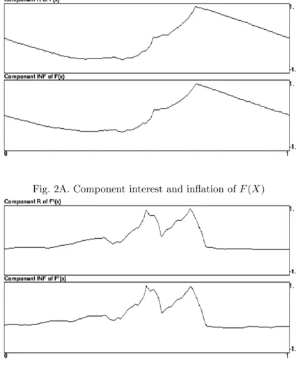
Figures 2A and 2B show the components of ˆF(x) and ˆF′(x), respectively, where a
common pattern among them is easily perceived, leaving ground for the possibility of a nonlinear co-trending between INF and R. Therefore, this work sticks to the conclusion thatg=1 at 10%;i.e., there is one co-trending vector.
3.3. VAR Results
Based on the previous results, three types of VAR were estimated: a) without any trend;
b) with a linear trend and
c) with Chebishev time polynomials.
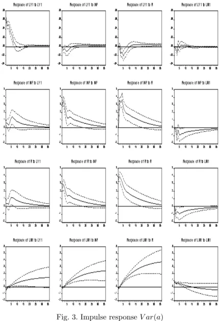
The Akaike, Hanan-Quinn and Schawarz information criteria were used to select lags. In case a) and b), 3 lags seems to be the best specification. Their impulse response analysis are very similar; that is, there is a inflation-puzzle that lasts for more than 20 months; and, as expected, there are some shocks with permanent effects, because the variables are not pure I(0) process. Figure 3 contains some of the plots of the impulse response analysis for the VAR without a trend.
time. Moreover, the inflation puzzle lasts only 7 months. Figure 4 presents these results.
Figure 4, also shows that output reacts negatively to a unit shock in the interest rate. The reduction reaches its maximum at the fourth month, something around 1.5%. Interest rate, by its turn, has been used to accommodate shocks in output, and reacts negatively to shocks in LM1. The impulse response of inflation rate to its own shock shows that its persistence has a 5 to 10 months duration.
There is an initial negative response of LM1 to interest rate shocks that becomes positive at the second month, differently from Rabanal and Schwartz (2001) which found a negative response. The initial negative response of LM1 to output, inflation and interest rate and its rise after some time elapses is what one could expected, in the sense that after some time LM1 is raised to keep the economy’s liquidity balance.
A shock on output causes a positive response of the inflation rate, and the interest rate seems to be used to stabilize output and inflation, while LM1 seems to be used only to maintain the economy’s liquidity. Most of these results are in tune with Minella (2001).
Using 3 lags and 20 Chebishev time polynomials for the innovation analysis, called as VAR(c.2), the effect of the interest rate on output lasts less than in the VAR(c.1), and its biggest impact happens in the second month. Again, there is an initial negative response of LM1 to interest rate shocks that becomes positive at second month, but it lasts only 8 months, when it then vanishes. LM1 really seems to be used to maintain the liquidity in the economy. The inflation puzzle was severely reduced to only 3 months, and much of the VAR(c.1) results was preserved under this new VAR, as presented in Figure 5.
4. Concluding Remarks
In this work a VAR was used to analyse the effects of monetary policy in Brazil. The fact that nonlinearities may cause some undesired effects on time series analysis was taken into account. Bierens (1997) shows that many series firstly looking as unit root processes could be, indeed, nonstationary with a nonlinear deterministic trend. Thus, using a VAR which takes into consideration these nonlinearities, all the sample could be used, instead of breaking it in small subsamples in order to avoid the undesirable effects of strucutural shifts to this kind of procedure.
Therefore, the entire sample data was submitted to both traditional and Bierens unit root tests. It seems that some of the series are neither pure unit root processes nor stationary or nonstationary with a deterministic trend. To be precise, the plots of INF, R and LM1 indicate that they have a nonlinear trend, and for LM1, Bierens’ test corroborates this feeling.
INF and R have a comovement and, as expected, this may cause a price-puzzle on VAR’s innovation analysis. Adding Chebischev time polynomials next to the intercept, most of the inflation puzzle was removed – it lasts then only 3 months. Cysne (2004), applying a VAR with bias-corrected confidence bands to Brazilian data, obtained a price-puzzle that lasts one quarter, also.
There are some possible reasons to explain why a co-trending does exists to INF and R. Brazil has experienced a long period of high inflation, and at that time all the prices in the economy were indexed. The past inflation was automatically transmitted to current prices, including the price of money – the interest rate. In July 1999, the Brazilian Central Bank adopted a inflation target regime using the interest rate, instead of LM1, as the main monetary instrument to control inflation, or expected inflation. This is captured by the impulse response analysis, where the interest rate was used to stabilize output and inflation, while LM1 reacts only to maintain the money balance.
It seems, therefore, that much of the positive response of inflation to a unit shock in the interest rate is due to the co-trending phenomenon between these two variables, and when the possibility of these nonlinearities in the data are considered, not only does the impulse response functions of the system become stationary, but also that the problem of inflation puzzle was severely diminished.
References
Bernanke, B. S. & Blinder, A. S. (1992). The federal funds rate and the channels of monetary transmission. American Economic Review, 82:901–921.
Bierens, H. J. (1997). Testing the unit root with drift hypothesis against nonlinear trend stationarity, with an application to the U.S. price level and interest rate.
Journal of Econometrics, 81:29–64.
Bierens, H. J. (2000). Nonparametric nonlinear co-trending analysis, with an application to interest and inflation rate in the U.S. Journal of Business & Economic Statistics, 18:323–337.
Cati, R. C., Garcia, M. G. P., & Perron, P. (1999). Unit roots in the presence of abrupt governmental interventions with an application to Brazilian data.Journal of Applied Econometrics, 14:27–56.
Christiano, L. J., Eichembaum, M., & Evans, C. (1994). The effects of monetary policy shocks: Evidence from the flow of funds. Working Paper Series 94-2, The Federal Reserve Bank of Chicago.
Cysne, R. P. (2004). Is there a price puzzle in Brazil? An application of bias-corrected bootstrap. Ensaios Econˆomicos 577, Funda¸c˜ao Getulio Vargas. Dickey, D. A. & Fuller, W. A. (1979). Distribution of the estimators for
autoregressive time series with a unit root. In Hamilton, J. D., editor, Time Series Analysis. Princeton University Press, Princeton.
Review, 36:1001–1012.
Kilian, L. (1998). Small-sample confidence intervals for impulse-response functions.
The Review of Economics and Statistics, 80:218–230.
Minella, A. (2001). Monetary policy and inflation in Brazil. Working Paper Series 33, The Central Bank of Brazil.
Pesaran, H. H. & Shin, Y. (1998). Generalized impulse response analysis in linear multivariate models. Economic Letters, 58:17–29.
Phillips, P. C. B. & Perron, P. (1988). Testing for a unit root in time series regression. Biometrika, 75:335–346.
Pope, A. L. (1990). Biases of estimators in multivariate non-gaussian autoregressions. Journal of Time Series Analysis, 11:249–258.
Rabanal, P. & Schwartz, G. (2001). Testing the effectiveness of the overnight interest rate as a monetary policy instrument. In Brazil: Selected Issues and Statistical Appendix. International Monetary Fund, Washington, D. C. IMF Country Report 01/10.
Appendix I
Fig. 2A. Component interest and inflation ofF(X)