330 Brazilian Journal of Physics, vol. 34, no. 1A, March, 2004
The Effects of Conserved Charges in a Nuclear Equation of State
B. Mattos Tavares
Instituto de F´ısica, Universidade Federal do Rio de Janeiro, 68528, 21945-970 Rio de Janeiro, RJ, Brasil
Received on 15 August, 2003.
We report the present status on the construction of an equation of state (EoS) for the strongly interacting mat-ter which is to be used in the hydrodynamical calculations for the ultra-relativistic heavy ion collisions. In the present version, the conservation of isospin, baryon number and strangeness are taken into account. A preliminary hydrodynamical result for our EoS, using the hydro code SPHERIO, is also shown.
1
Introduction
If the local thermal equilibrium is attained in relativistic heavy ion reactions, hydrodynamical description may be most adequate for the space-time evolution of the system. It is a very powerful method [1]. Once the initial condition (spatial distribution of 4-velocity field and conserved cur-rents) of the system is specified, the subsequent dynamics is determined uniquely by the EoS of the matter composing the system. Therefore, we expect that a systematic analy-sis of the experimental observables related to the collective dynamics of the system in terms of the hydrodynamical de-scription will offer the important information on the EoS, namely, the thermal properties of the QGP and hadronic matter. For such purposes, it is essential to provide the equa-tion of state in terms of an efficient computaequa-tional procedure which supplies all the thermodynamical quantities, temper-ature, chemical potentials, pressure, etc., as functions of the two independent variables of the hydrodynamical calcula-tion, for example, the baryon number density and entropy density. It is also desirable to establish a method to adapt the EoS easily to the changes of various physical model pa-rameters in order to study the effects of these changes in the hydrodynamical evolution of the system. In this work, a method of construction of the EoS is developped and some results are reported.
2
The equation of state
In the NEXUS+SPHERIO program [2], the initial condition is provided by the event generator NEXUS, based on the Gribov-Regge model[3] of hadronic collisions. This pro-gram generates, in event-by-event basis, the spatial distri-bution of the energy-momentum tensorTµνand the baryon
number density nB on the hypersurface τ = const.
As-suming that the system reaches the local thermal equilib-rium, we then obtain the initial energy and temperature dis-tribution using the EoS for QGP and relativistic hadronic gas. The subsequent dynamical evolution is followed by the
SPHERIO1code.
Following the works in ref. [5, 6, 7], the present EoS assumes the plasma and hadronic phases as a gas of ideal relativistic quantum particles. It exhibits a first order phase transition between the two states as shown below.
2.1
Relativistic ideal gas, particle mixture
and conserved charges
For a grand-canonical ensemble of ideal-quantum particles the pressure is given by
P= θg (2π)3
Z
d3k ln(1 +θeβ(µ−ǫk)
) (1) wereθ=1 for fermions (and -1 for bosons),βis the inverse of temperature,µis the chemical potential,gis the degener-acy factor andǫk =
√
k2+m2is the dispersion relation for
the particle wheremis the mass of the particle.
The densitynand the energy densityecan be obtained by the usual thermodynamical relations, n = ³∂P
∂µ
´
V,T,
e=³∂P ∂β
´
λ, whereλis the fugacity. The entropy density of
the gas can be calculated ass=β(P+e−µn).
When we include conserved charges such as isospin (3rd
component), baryon number and strangeness, the chemical potential [8] must be written asµ =BµB+SµS +T3µ3
whereB, S, T3are baryon, strangeness and isospin quantum
numbers, respectively andµB, µS, µ3are the corresponding
chemical potentials.
2.1.1 Gas of Quarks and Gluons
For simplicity, in our EoS we treat the plasma phase as an ideal gas of relativistic quarks and gluons plus the vacuum pressureB.
Considering the mixture of flavors, the total pressure is given by the expression
PQGP(T,{µi}) =PQuarks(T,{µi}) +PGluons(T)−B
B. Mattos Tavares 331
HerePQuarks is already a sum of individual (u,d,s) quark
pressures (each one given by eq.(1)), B is the bag constant to simulate confinement properties andµi=BiµB+SiµS+
T3,iµ3; i=(u,d,s). For gluons we have used eq.(1) withµ=
0. Analogously energy density is given by:
eQGP(T,{µi}) =eQuarks(T,{µi})+eGluons(T)+B (3)
And entropy density for the Plasma is
sQGP(T,{µi}) =sQuarks(T,{µi}) +sGluons(T) (4)
For the total densities we have only
nQGPk (T,{µi}) =nkQuarks(T,{µi}) ; k=B, S,3 (5)
because gluon density is zero.
2.1.2 Gas of Hadrons
Basically we treat the hadronic phase as a mixture of gases of quantum relativistic particles, except for the excluded vol-ume effect, like a Van der Waalls hard core correction [6, 7], to fit the densities to the data. In this case, we have:
Pexcl= h
X
t=1
Pid
t (T,µ˜t) ; µ˜t≡µt−vtPexcl (6)
whereµt=BtµB+StµS+T3,tµ3is the chemical
poten-tial of the t-th hadron specie ,his the maximum number of hadrons considered andvtis the excluded volume of the t-th
hadronic species. Pexclis determined iteratively. Forn k,e
andsof the t-th hadronic species (k=B,S,3 as before) we have:
Qexclt =
Qid t
1 +Ph
i=1vinidi (T,µ˜i)
(7) whereQ= nk,eor s. The superscriptid means ideal, so
it should be calculated as in the section 2.1. To get the to-talnk,eorsof the hadron gas (HG), we must sum over the
hadrons. In the present calculation, we took the bag constant B = 380M eV /f m3 and excluded volumev0 = 4πR30/3
for baryons (with R0 = 0.7f m) and v0 =0 for mesons,
as done in [6]. Other possibilities for excluded volume (e.g ref.[5]) will be explored in future works. All known mesons with mass under 2 GeV and baryons with mass un-der 2.5 GeV were included in calculations [9]. We took quark massesmu=1.5 MeV,md=3.0 MeV andms=120.0
MeV, although the light quark masses are irrelevant in our EoS.
2.2
The phase transition
To construct our phase diagram, we determine the phase boundary using Gibbs equilibrium condition[10] between the QGP and HG phases, i.e. we require thermal, mechani-cal and chemimechani-cal equilibrium (forµBonly) during the phase
transition. In the present work, we only consider the case where strangeness and isospin vanishes, thus, the chemical
potentialsµS andµ3are determined by(T, µB). Some
ex-amples of our numerical phase diagrams can be found in Figs. 1 and 2.
Figure 1. Phase diagrams for T andµB.
Figure 2. A phase diagram in (s, nB) plane.
Recent lattice calculations [11] indicate that there is a second order “end point” at non zeroµB, and between this point andµB = 0 the transition should be a smooth cross over[12]. Our simple treatment does not have this feature. It maybe interesting to find a simple parametrization of the equation of state, for instance, in terms of the variation of the bag constant as a function of the temperature and chemical potencial, to simulate the appearance of the critical point.
3
Numerical procedure and Results
In order to permit a hydro code to give reliable outputs within a reasonable time of calculation, the numerical EoS must furnish the thermodynamical quantities in a precise and fast way. Specifically in our hydro code SPHERIO, for a given (e, nB) at the initial condition or (s, nB) during the dynamical evolution of the system, the EoS need to supply
332 Brazilian Journal of Physics, vol. 34, no. 1A, March, 2004
the freeze-out time, in order to compute single particle dis-tributions using the Cooper-Frye procedure.
To achieve these purposes, we adopted the following procedure. First, we constructed a set of large numerical tables for the thermal quantities as functions ofT, µB. This
has been done evaluating numerically thermal integrals im-posing conservation of strangeness and isospin. That is, µS, µ3 are determined as functions ofT, µB. These tables
are too large to be used directly in the hydro code. Thus, the values of these tables are fitted by domain-wise quadratic functions in (T, µB) and the coefficients of these quadratic
functions are stored. In the routine used in hydro code, any
output quantity can be obtained by a quadratic interpola-tion for a giveninput(e, nB) or (s, nB). The total number
of domains in the present version is around 16000 (6000 for hadronic region and 10000 for QGP). For each thermo-dynamical quantity, we need to store 6 coefficients per do-main. We have done a landmark check for these functions, and it took approximately 2 minutes for 500000 points in a rather modest PC (pentium-pro 800Mhz, with 512 MB RAM) which we consider satisfactory.
The quadratic interpolation applied here is very precise and effective, provided that the size of interpolation domain, in the (T, µB) plane, is small enough. In degenerated
re-gion, the convergence condition becomes more severe so that some special care should be taken. In the final form of the subroutines we constructed, the error between a given Qand recalculatedQc (whereQ = e, sor nB ) using the
original thermal integrals is less than 0.01%. In low tem-perature regions, where the validity of our procedure is not guaranteed, the error can achieve 30%. But we know hy-drodynamics rarely achieve these regions, where the hydro procedure becomes to fail. Otherwise a more precise table can easily be constructed.
In the mixed phase we use a linear interpolation between the two points on the phase boundaries of QGP and hadronic gas with the sameT, µB, P. Writingα, the fraction of the
hadronic component in the mixed phase, any thermal quan-tity is given as Qint = αQHG+ (1−α)QQGP (where
Q= (e, nB, s)). The error in these phase is less than 0.01%
everywhere.
To compute numerically the thermal integrals we have used the Gauss-Laguerre quadrature method [8] which works quite well in most ofT, µvalues. However, in ex-tremely degenerate domain, both for fermions and bosons, the method is not adequate. There, the asymptotic formula for the fermions are used instead. For bosons, to avoid the singularity at (µ→m) we modified the singular denomina-tor by an exponentially increasing, but still regular function. The phase boundaries of the system, necessary for phase judgement of the input point, was computed numerically us-ing Newton method for solvus-ing the phase equilibrium equa-tions. Our calculation is good for the temperature higher than 25 MeV. Below this temperature, the hadronic gas inte-grals are not accurate enough to solve the phase equilibrium conditions numerically. Thus, our equation of state is ap-plicable only forT ≥26M eV. This will not be a problem since the hydrodynamical procedure is not valid for such low temperatures, as mentioned before.
Analyzing Fig. 1 we note that inclusion of isospin and strangeness conservation enlarges the hadronic domain in (T, µB) plane compared to the equation of state which does
not account for these quantum numbers. The inclusion of quark masses does not affect much the form of the phase diagram (only a little inTc(µB = 0)). Change of the bag
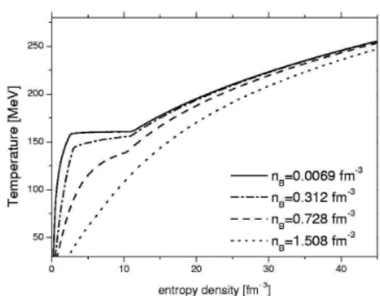
constant B directly affects the critical temperature at the µB = 0. In Fig. 3 we show the behavior of temperature
as function of entropy density for variousnB =const, and
we can see that it is a continuous function as should be.
Figure 3. Temperature versus entropy density for various baryon densities.
4
Conclusions and Perspectives
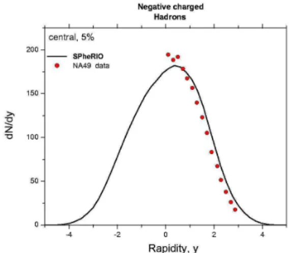
In this report, we presented the method of construction of the equation of state used in the hydrodynamical code and a preliminary version of the EoS with strangeness and charge conservation. There are still some points to be improved, but the overall properties are satisfactory. To show how works the present routine of the equation of state, we incorporated it to the SPHERIO code and calculated an example of rel-ativistic nuclear collision. In Fig. 4 we show the result for a rapidity distribution of negative charged hadrons, gener-ated from SPHERIO code, for a single event. The initial condition was given by the NEXUS event generator, corre-sponding to a 5% most central Pb+Pb collision at energy of √
s= 17.3 AMeV. The freeze-out temperature was taken to be 140 MeV.
B. Mattos Tavares 333
Figure 4. Rapidity distribution for charged hadrons at SPS ener-gies. The dots are experimental data, and the full line is the numer-ical result.
The present report is a part of the work done in collab-oration with Profs. C. E. Aguiar, T. Kodama, Y. Hama, F. Grassi and Dr. O. Scolowski. The author expresses his thanks to Drs. P. Lotti and M. Makler for their kind help. This work is supported by CNPq, FAPERJ, CAPES and FAPESP.
References
[1] See for example P. Huovinen, nucl-th/0305064; P.F. Kolb and U. Heinz, nucl-th/0305084.
[2] For the union of NEXUS with SPHERIO see, for example, Nucl. Phys A698, 639c (2002).
[3] H.J. Drescheret al, Phys Rev. C65, 054902 (2002).
[4] For SPH procedure in RHIC see C.E. Aguiar, et al. J. of Phys. G27, 75 (2001).
[5] B. Muzingeret al., Phys. Lett. B465, 15 (1999).
[6] C.M. Hung, E. Shuryak, Phys. Rev. C57, 1891 (1997).
[7] G.D. Yen, M.I. Gorenstein, W. Greiner, and S.N. Yang Phys Rev. C56, 2210 (1997).
[8] T. Kodama, p.3, New states of matter in hadronic interac-tions, PASI proceedings, AIP (2002).
[9] Particle data, Phys. Rev. D45, (1992)
[10] J. Sollfrank and U. Heinz, nucl-th/9505004.
[11] Z. Fodor and S.D. Katz, hep-lat/0106002.
[12] K. Rajagopal, hep-ph/0009058.