Inflation and Precision Cosmology
J´erˆome Martin
Institut d’Astrophysique de Paris,GRεCO–FRE 2435, 98bis boulevard Arago, 75014 Paris, France
Received on 18 December, 2003
A brief review of inflation is presented. After having demonstrated the generality of the inflationary mechanism, the emphasis is put on its simplest realization, namely the single field slow-roll inflationary scenario. Then, it is shown how, concretely, one can calculate the predictions of a given model of inflation. Finally, a short overview of the most popular models is given and the implications of the recently released WMAP data are briefly (and partially) discussed.
1
Introduction
The inflationary scenario [1] has been invented in order to solve and explain some observational facts (isotropy of the Cosmic Microwave Background Radiation–CMBR–, flat-ness of the space-like sections, etc . . . ) that could not be properly understood in the context of the standard hot Big Bang theory. Therefore, at the beginning of its history, the inflationary scenario was only able to make postdictions but, given the problems of the standard model at that time, this was already a success. However, soon after its advent, it was realized [2, 3] that inflation, when combined with quantum mechanics, can also give a very convincing mechanism for structure formation. In particular, for the first time, it was understood how to generate a scale-invariant power spec-trum. Therefore, the inflationary mechanism was able to establish a beautiful connection between facts which, be-fore, were considered as independent. However, since the Harisson-Zeldovich was already known to be in agreement with the observations, it could be argued that, somehow, this was again a postdiction. In fact, the inflationary scenario does not predict a scale invariant spectrum but a nearly scale invariant spectrum, the deviations from the scale invariance being linked to the microphysics description of the theory. This constitutes a definite prediction of inflation that can be tested [4].
Slightly more than twenty years after the invention of inflation, the situation has recently changed because, thanks to the high accuracy CMBR data obtained, among others, by the WMAP satellite [5], we can now start to probe the details of the inflationary scenario and check its predictions. The goal of this short review is, after having tried to jus-tify why the inflationary mechanism is generic (section I), to show how, in its most popular and simplest realization, one can calculate concrete predictions (section II) and com-pare them with the recent observations (section III). These proceedings, due to the lack of space, do not cover many important topics. Among them and since this is particularly relevant for the present article, we just would like to signal the discussion of why the presence of the CMBR Doppler
peaks strongly suggests that a phase of inflation took place in the early universe, see Ref. [6].
2
The inflationary mechanism
2.1
Basic equations
The cosmological principle implies that the universe is, on large scales, homogeneous and isotropic. This simple as-sumption drastically constrains the possible shapes of the Universe which can solely be described by the Friedman-Lemaˆıtre-Robertson-Walker (FLRW) metric:ds2=−dt2+
a2(t)γ(3)
ij dxidxj, where γ (3)
ij is the metric of the three-dimensional space-like sections of constant curvature. The time-dependent functiona(t)is the scale factor. If the spa-tial curvature vanishes then γ(3)ij = δij, where δij is the Kr¨onecker symbol. The previous expression is written in terms of the cosmic timetbut it is also interesting to work in terms of the conformal timeη defined bydt =a(η)dη. Then, the metric can be re-expressed as
ds2=a2(η)−dη2+γij(3)dxidxj. (1)
In terms of conformal time, the Hubble parameterH = ˙a/a
can be written asH =H/awhereH ≡a′/a, a dot deno-ting a derivative with respect to cosmic time while a prime stands for a derivative with respect to conformal time.
Matter is assumed to be a collection ofN perfect fluids and, as a consequence, its stress-energy tensor is given by the following expression
Tµν = N
i=1
Tµν(i)= (ρ+p)uµuν+pgµν, (2)
relation uµuµ = −1. In terms of cosmic time this me-ans thatuµ = (1,0)whereas in terms of conformal time one has uµ = (1/a,0) andu
µ = (−a,0). The fact that the stress-energy tensor is conserved,∇αT
αµ = 0, implies
ρ′ + 3H(ρ+p) = 0. This expression is obtained from the time-time component of the conservation equation. The time-space and space-space components do not lead to any interesting equations for the background.
We are now in a position to write down the Einstein equations which are just differential equations determining the scale factor. In terms of cosmic time, they read
˙
a2
a2 +
k a2 =
κ
3ρ , −
2¨a
a+
˙
a2
a2 +
k a2
=κp , (3)
whereκ≡8πG= 8π/m2
Pl,mPlbeing the Planck mass and wherek = 0,±1is the normalized three-dimensional cur-vature. Combining the two expressions above, one obtains an equation which permits to express the acceleration of the scale factor¨a/a=κ(ρ+ 3p)/6. From the above equation, one sees that any form of matter such thatρ+ 3p <0will cause an acceleration of the scale factor (this is only true, of course, if the matter component satisfyingρ+ 3p <0is the dominant one). The energy density is always positive but, in some situation, the pressure can be negative and the inequa-lityρ+ 3p < 0may be realized. This simple remark is at the heart of the inflationary scenario. Let us notice that the above property is deeply rooted into the fundamental prin-ciples of general relativity. It is because all forms of energy weighs in general relativity that the pressure participates to the equation giving the expression of¨a. This has to be con-trasted with Newtonian physics where the same expression reads¨a/a = −κρ/6,i.e. only the energy density affects the expansion. As a consequence, the expansion can only be decelerated.
A class of solutions of particular interest is that for which the equation of stateω≡p/ρis a constant. In this case, the conservation equation can be immediately integrated and le-ads to ρ ∝ a−3(1+ω). Then, the scale factor is given by a power law either of the conformal or of the cosmic time, namely
a(η) =ℓ0|η|
1+β, a(t) =a 0
t t0
p
, (4)
where the sign of the conformal and cosmic times, to be discussed below, can be negative or positive. The parame-ters p and β are related by β = (2p−1)/(1−p) and
p = (1 +β)/(2 +β). The link between ωand the para-metersβandpcan be expressed as
ω= 1−β
3(1 +β) =−1 + 2
3p. (5)
The casesβ =−1and/orp= 0are obviously meaningless since they do not correspond to a dynamical scale factor.
Let us now come back to the question of the sign of the conformal and cosmic times. For the class of models under consideration, the Hubble parameter can be easily calcula-ted and is given byH =p/t. Let us first consider the case where we have an expansion,i.e. H > 0. In this case, one
hast > 0for p > 0 andt < 0for p < 0. On the other hand, in the case of a contraction,H <0, we havet >0for
p <0andt <0forp >0. The link between the two times,
dt=adη, takes the form
η = 1
a0(1−p)
|t|1−p,
if t >0, (6)
η = −1
a0(1−p)
|t|1−p,
if t <0, (7)
from which we deduce that, ift >0, thenη <0forp >1
andη >0forp <1and that, ift <0, thenη >0forp >1
andη <0forp <1.
Finally, let us also examine some cases of particular in-terest. The casep= 2/3corresponds to an expanding mat-ter dominated universe and ω = 0. Therefore, we have
η >0andt >0. The same conclusion applies for the case
p= 1/2,i.e. the case of an expanding radiation dominated universe withω = 1/3. The caseβ = −2corresponds to
p=∞, that is to say to an exponential scale factor: this is just the de Sitter solution withω =−1. Forβ <−2, one hasp >1andη <0,t >0if we are interested in the case of expansion.
The evolution of the background space-time can be very roughly understood by means of the previous set of sim-ple equations. The hot Big Bang model before the advent of inflation just consisted into a radiation dominated epoch (ω = 1/3) taking place at high redshifts, untilzeq ≃ 104, followed by a phase dominated by cold matter (ω = 0). However, already at this level, this very simple framework leads to unacceptable conclusions. We now describe what are (some of) the problems of the pre-inflationary hot Big Bang scenario and how postulating a new phase of accele-rated expansion in the very early universe can avoid these problems.
2.2
The horizon problem
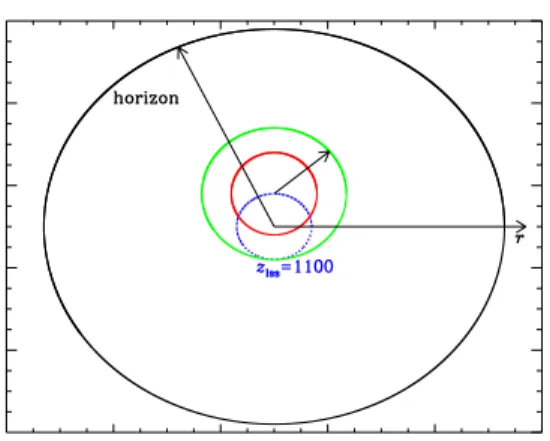
The horizon problem consists in the following. The furthest event that we can directly “see” in the universe is the (re)combination, i.e. the time at which the electrons and the protons combined to form hydrogen atoms. Since the photon–atom cross-section (Rayleigh cross-section) is much smaller than the photon–electron cross-section (Thomson cross-section), the universe became transparent at that time. The COBE [7] and WMAP [5] maps of the sky are pho-tographs of the universe at this epoch. The recombination took place at a redshift ofzlss≃1100,i.e.within the epoch dominated by the cold matter. Before, the universe was opa-que and therefore it is not possible to observe it directly at earlier times from the Earth. Since no physical process can act on scales larger than the horizon (see below for a precise definition of the horizon), we typically expect the universe to be strongly inhomogeneous on those scales. Seen from the Earth, this means that the COBE map should look ex-tremely different on angular scales larger than the angular scale of the horizon at recombination.
at recombination, seen by an observer today. Roughly spea-king, this is just the size of the horizon at the last scattering surface divided by the present (angular) distance to the last scattering surface. In other words, it can be expressed as
∆Ω = dH(tlss)/dA(tlss), where we now discuss precisely the meaning of the terms in the above formula.
For this purpose, it is convenient to choose the coordi-nates system such that the origin is located on Earth, i.e.
such that “our” co-moving coordinate is r = 0. Suppose that a photon is emitted at spatial co-moving coordinates
(rem, θem, ϕem)and at cosmic timetem. The path followed by the photon can be chosen such thatθ=cst.andϕ=cst since this is a solution of the geodesic equation. In this case, the path is completely characterized by the function
r=r(t). This quantity is given by
r(t) =rem− t
tem
dτ
a(τ) ⇒dP(t) =a(t)
rem− t
tem
dτ a(τ) ,
(8) wheredP(t)is the physical (proper) distance from the “po-sition” of the photon at timetto the origin.
This equation can be used to define the horizon. Indeed, the question that one may ask is the following. At a given (reception) time,t=trec, what is the proper distance to the furthest point where a photon, sent to us from there, could have reached the Earth (the point of co-moving coordinate
r = 0) before or at the timetrec? This proper distance is called the size of the horizon at timet = trec. Clearly the distance is maximized if the time of emission is the Big-Bang and if the photon has just reached the Earth at the time
trec. Hence the co-moving coordinate of emission is obtai-ned by writing thatdP(trec) = 0and by taking a vanishing lower bound in the previous integral. This implies that
rem= trec
0
dτ
a(τ). (9)
This means that the distance to the horizon, at the time
t = trec, is given bydH(trec) = a(trec)rem. In this equa-tion,treccan be for instance the time of recombination,tlss or the present timet0depending on whether one wants the evaluate the size of horizon at the last scattering surface or now.
Another question is to calculate the distance to a point where a photon emitted att=temhas just arrived on Earth now, at timet = t0. Writing again that the photon is re-ceived now, one obtains the corresponding co-moving coor-dinate of emissionrem=ttem0 dτ /a(τ). From the previous equation, one can deduce that the corresponding angular dis-tance to the point of emission is given bydA ≡a(tem)rem. Indeed, the FLRW metric can be written as (for flat space-like section)ds2=−c2dt2+a2(t)(dr2+r2dΩ22)and the-refore the proper distanceDacross a source isD ≃ar∆Ω
at timetem(obtained fromdt= dr= 0since it is supposed that the source is located on a sphere of radiusr=cte). As a consequence, one has∆Ω = D/(ar)from which we de-ducedA ≡a(tem)r(tem). Notice that the proper distance to the point of emission isa(t0)rem. For very high redshifts, as for instancezlss, these two distances are of course very different.
We can now deduce the general expression of the angu-lar diameter. It is given by
∆Ω =
tlss 0
dτ a(τ) ×
t0 tlss
dτ a(τ)
−1
. (10)
In the previous expression, the factorsa(tlss)have canceled out.
Let us now try to evaluate the above solid angle in a re-alistic case where matter and radiation are present [8]. For simplicity, we assume that the universe is radiation domi-nated before recombination and matter domidomi-nated after. In reality, as already mentioned, equivalence between radia-tion and matter takes place before the recombinaradia-tion but this does not introduce important corrections. Since we are going to study the influence of a phase of inflation, we also assume that the epoch dominated by radiation can be inter-rupted during the periodti< t < tend. During this interval, we assume that the universe is dominated by an unknown fluid the equation of state of which is constant and given byωX. To recover the standard hot Big Bang case, where this epoch does not occur, it is sufficient to consider that
ti=tend,i.e.to switch off the phase dominated by the unk-nown fluid. The scale factor is not kunk-nown exactly but its piecewise expression reads:
⌋
a(t) = ai(2Hit)1/2, 0≤t < ti, a(t) =ai 3
2(1 +ωX)Hi(t−ti) + 1
2/[3(1+ωX)]
, ti≤t < tend, (11)
a(t) = aend[2Hend(t−tend) + 1]1/2, tend≤t < teq, a(t) =aeq 3H
eq
2 (t−teq) + 1
2/3
, teq≤t < t0.(12)
At each transitions, the scale factor and its first time derivative are continuous. A straightforward calculation leads to the expressions of the horizon at decoupling and of the angular distance to the last scattering surface. One finds
dA(tlss) = alss t0
tlss
dτ
a(τ) =alss× 2
a0H0
1−
a lss
a0 1/2
, (13)
dH(tlss) = alss tlss
0
dτ
a(τ) =alss× 1
a0H0 a
lss
a0 1/2
1 + 1−3ωX
1 + 3ωX
aend
alss
1−
a
i
aend
(1+3ωX)/2
From the aboves equations, we deduce the expression of the solid angle
∆Ω = 1 2
1−(1 +zlss)−1/2 −1
(1 +zlss)−1/2
1 +1−3ωX
1 + 3ωX
1 +zlss
1 +zend
1−e−N(1+3ωX)/2 ,
(15)
⌈
whereN ≡ ln(aend/ai) is the number of e-foldings du-ring inflation andzendis the redshift at which inflation stops (corresponding tot=tend).
Let us first suppose that there is no phase of inflation,
i.e.N = 0. Then,∆Ω≃0.5×(1 +zlss)−1/2≃0.85◦. As a consequence, one expects the last scattering surface to be made of≃1◦ patches whose physical properties are com-pletely different (let us remind that the angular diameter of the moon seen from the Earth is≃0.5◦). This is obviously not the case: up to tiny fluctuations of orderδT /T ≃10−5, the CMB radiation is extremely homogeneous and isotro-pic. This paradox is called the horizon problem. A solution to this problem is to assume that the initial conditions were identical in all the causally disconnected patches but this se-ems very difficult to justify. Another solution is to switch on the inflationary phase. To significantly modify the solid angle in Eq. (15), the unknown fluid responsible for infla-tion must have an equainfla-tion of state such thatωX <−1/3. Indeed, if1 + 3ωX >0, then the argument of the exponen-tial in Eq. (15) is negative and the correction coming from the phase driven by the unknown fluid becomes negligible. On the other hand, if1 + 3ωX <0, then the correction can be very important, depending of course on the value of the
number of e-foldsN. Writing that the last scattering surface looks very isotropic, that is to say∆Ω>4π, allows us to put a constraint on this quantity. One obtainsN−4+lnzend. Notice that it is necessary to assume thatωX is not too close to−1/3otherwise terms like1 + 3ωX, that we have neglected, could also have an effect on the constraint derived above.
Let us now try to better understand and to physically in-terpret what has been done. This is summarized in Fig. 1 that we now describe in more details. The proper distance to the last scattering surface is given by
dlss=a0 t0
tlss
dτ a(τ) =
2
H0
1−
alss
a0 1/2
. (16)
This is approximatively the Hubble distance today, defi-ned by ℓH ≡ H
−1
0 , since we have dlss ≃ 2H0−1 ≃
6000h−1Mpc ≃ O(1)ℓ
H where we have used H0 ≡
100hkm s−1Mpc−1
. Obviously, this number does not de-pend on the fact that there is a phase of inflation or not. On the other hand, the size of the horizon today is given by the following expression
⌋
dH(t0) =a0 t0
0
dτ
a(τ) = a0× 1
a0H0
alss
a0 1/2
1 +1−3ωX
1 + 3ωX
aend
alss
1−
ai
aend
(1+3ωX)/2
+a0× 2
a0H0
1−
alss
a0 1/2
. (17)
⌈
If there is no phase of inflation (or if1 + 3ωX >0) then one hasdH(t0)≃2H−
1
0 ≃dlss≃ℓH. This is why, in the left pa-nel in Fig. 1, the (black) horizon and the (blue) last scattering surface have about the same size. The horizon at recombi-nation has been calculated in Eq. (14). If there is no phase of inflation then one hasdH(tlss)≃H
−1
0 (1+zlss)−3/2≪dlss. This is why in the left panel in Fig. 1, the red and the green
Figure 1. Left panel: Sketch of the evolution of the horizon. The origin of the coordinates is chosen to be Earth. The red circles represent the size of the horizon at the time of equality,zeq≃104. The green circles represent the horizon at the time of recombinationzrec≃1100. The black circle represents the horizon today. The dotted blue circle represents the surface of last scattering viewed from Earth. The angle∆Ω
is the angular size of the horizon at recombination viewed from Earth. Right panel: Sketch of the evolution of the horizon in an inflationary universe. The conventions are the same as in the left panel. The horizon at recombination now includes the last scattering surface and there is no horizon problem anymore.
Let us now turn to the inflationary solution and the right panel in Fig. 1. The proper distance to the last scattering surface is not modified. But, and this is the crucial point, the size of the horizon is now completely different. Using Eq. (14), with now1 + 3ωX <0, we obtain
dH(tlss)≃
1
H0
(1 +zlss)−3/2
1 + zlss
zend a
end
ai ≫
dlss.
(18) This is why in the right panel in Fig. 1 the (green) ho-rizon now encompasses the (blue) last scattering surface. Another consequence is that the (black) horizon today is now much bigger than the Hubble scale which, as already mentioned, is still approximatively equal to the size of the blue last scattering surface. For the purpose of illustration let us take the example of chaotic inflation. In this case we havezend≃1028andaend/ai ≃exp(1028)from which we deduce that (!) dH(t0) ≃3×10
43429421h−1Mpc. Clearly this scale is totally different from the Hubble scale and, in the context of an inflationary universe, one should carefully make the difference between those two scales.
2.3
The flatness problem
This problem becomes more apparent if the Friedman equa-tion is cast into a different form. Let us define the parameter
Ωi, which gives the relative contribution of the fluid “i” to the total amount of energy density present in the Universe, byΩi(t) ≡ ρi(t)/ρcri(t), where the critical energy density isρcri ≡ 3H2/κ. This last quantity is nothing but the to-tal energy density of a universe with flat space-like sections. This is a time-dependent quantity. The Friedman equation takes the formk/(a2H2) =N
i=1Ωi(t)−1≡ΩT(t)−1. The parameter ΩT(t) directly gives the sign of the curva-ture of the space-like sections. Sincekis not a function of time, the sign ofΩT−1cannot change during the cosmic evolution. In general, it is difficult to solve the differential equation giving the time evolution ofΩT(t) and to obtain the explicit time dependence ofΩT. However, it is possible to expressΩT in terms of the scale factora(t), at least in the case where all the fluids have a constant equation of state parameter. One obtains
⌋
ΩT(a) = N
i=1
Ωi(t0)
a a0
−3(1+ωi)
N
j=1
Ωj(t0)
a a0
−3(1+ωj)
−[ΩT(t0)−1]
a a0
−2
−1
. (19)
If one assumes that only radiation and matter are present then, asa/a0goes to zero, it is clear that radiation becomes dominant. In this case, a good approximation of the previous equation is
ΩT(t)−1≃
ΩT(t0)−1
Ωrad(t0) a
a0 2
= ΩT(t0)−1
Ωrad(t0)
1
z+ 1
2
.
(20) Today it is known that |ΩT(t0)−1| < 0.1. This clearly means that, at high redshifts, the quantity|ΩT(z)−1|was extremely close to zero. For instance, at the redshift of nu-cleosynthesis, znuc ≃3×10⁸, one has|ΩT(znuc)−1| ≃
O(10−14) where we have taken Ω
rad(t0) ≃ 10−4. It is difficult to understand why this quantity was so fine-tuned in the early Universe. At Grand Unified Theory (GUT) scale (zGUT ≃ 10
28), the constraint becomes even worse
|ΩT(zGUT)−1| ≃ O(10−
52). To explain this fact, we have two possible solutions: (i) we simply assume that the ini-tial conditions were fine-tuned in the early Universe or (ii) we find a mechanism which automatically produces such a small value at high redshifts. Since, as already mentioned for the horizon problem, the first explanation seems artifi-cial, let us concentrate on the second one. Thus, we assume that, for redshiftsz > zend, the Universe was dominated by another type of matter, different from matter or radiation. As before, we simply characterize this unknown fluidX by its equation of stateωX. The equation of state should be chosen such that, from any reasonable (i.e. not fine-tuned) initial conditions in the very early Universez ≫zend, it automa-tically produces aΩT −1close to zero, with the required accuracy atz=zend.ΩTcan be written as
ΩT(a) =
ΩX(ai)
ΩX(ai) + [1−ΩT(ai)] a
ai
1+3ωX , (21)
where ai is the value of the scale factor at some initial redshiftzi. Sinceaend/ai≫1, the conditionΩT(aend)≃1 is clearly equivalent to1 + 3ωX <0. Then, from any initial conditions atz =zi, the value ofΩT(aend)will be pushed toward one as long asXdominates. Therefore, one recovers the fact that a fluid with a negative equation of state parame-ter can solve a problem of the hot Big Bang model. One can even derive the constraint that the parameters describing the epoch dominated by the fluidX must satisfy. If one re-quires thatΩT has been pushed so close to one during the phase dominated byXthat the remaining differenceΩT−1 will not sufficiently increased during the radiation and do-minated epochs to compensate the first effect and to be dis-tinguishable from zero today, one arrives at [from Eqs. (20) and (21) written atz=zend]
aend
ai
1+3ωX
= eN(1+3ωX)104×z−2
end, (22)
which can also be expressed asN −4 + lnzend, where we have assumed for simplicity that|1 + 3ωX| =O(1). It is quite remarkable that this constraint be the same as the one derived from the requirement that the horizon problem is solved. To conclude, let us give some numerical exam-ples: forzend ≃1010,i.e. two orders of magnitude above
nucleosynthesis, one hasaend/ai ≃108that is to say≃19 e-foldings. Forzend ≃zGUT, one obtainsaend/ai ≃10
26, namely≃60e-foldings.
The main lesson of the previous calculations is that, as-suming an epoch in the early Universe dominated by a fluid the equation of state parameter of which is negative, provi-des an elegant way to solve the problems of the standard hot Big Bang model. Here, the important point is that the detai-led properties of the unknown fluid and/or its physical nature are unimportant, at least at the background level, provided the equation of state parameter is negative. This makes the inflationary solution quite generic.
2.4
Single scalar field inflation
We have seen in the previous sections that inflation can be caused by any fluid such thatρ+ 3p <0. We now discuss a concrete realization of the inflationary mechanism. Infla-tion is supposed to take place in the very early universe, at very high energies. At those scales, the fluid description of matter is not expected to hold anymore and (quantum) field theory seems to be the most appropriate way to describe the behavior of matter. The simplest example, compatible with the symmetries of the FLRW metric, is a scalar fieldφ0(η). This field will be called the inflaton in what follows. The corresponding Lagrangian reads
S=−
d4x√−g
1
2g
µν∂
µφ0∂νφ0+V(φ0) , (23)
whereV(φ0)is the potential,a prioria free function but we will see that, in order to have a successful inflationary phase, its shape must satisfy some constraints. The stress-energy tensor can be written as
Tµν =∂µφ0∂νφ0−gµν
1 2g
αβ∂
αφ0∂βφ0+V(φ0) . (24)
From this expression, one sees that the scalar field can also be viewed as a perfect fluid. The energy density and the pressure are defined according toT0
0=−ρandTij =pδij and read
ρ=1 2
(φ′ 0)
2
a2 +V(φ0), p=
1 2
(φ′ 0)
2
a2 −V(φ0). (25) The conservation equation can be obtained by inserting the previous expressions of the energy density and pressure into the equationρ′+ 3H(ρ+p) = 0. Assumingφ′
0 = 0, this reproduces the Klein-Gordon equation written in a FLRW background, namely
φ′′ 0 + 2
a′
aφ
′ 0+a
2dV(φ0)
dφ0
= 0. (26)
kinetic energy dominates the potential energy whereω≃1,
i.e. the case of stiff matter or, on the contrary, when the po-tential energy dominates the kinetic energy for which one obtainsω≃ −1. This last case is of course the most interes-ting for our purpose. This shows that inflation corresponds to a regime where the potential energy dominates the kinetic energy:V(φ0)≫(φ′0)
2, see Eqs. (25). We also note in pas-sing that an equation of statep≃ −ρimplies that the energy density of the field will be almost constant during inflation. The fact that the kinetic energy is small during inflation me-ans that the potential should be very flat which is the main requirement for a successful model of inflation if this one is
caused by a scalar field.
In general, the equations of motion can be integrated exactly only for a very restricted class of potentials. On the contrary, one would like to able to characterize this mo-tion for any given, sufficiently flat, potentials. To reach this goal, we clearly need a scheme of approximation. Since the kinetic energy to potential energy ratio and the scalar field acceleration to the scalar field velocity ratio are small, this suggests to view these two ratios as parameters in which a systematic expansion is performed. The slow-roll motion of the scalar field is controlled by the three “slow-roll parame-ters” (at leading order, see e.g. Ref. [9]) defined by:
⌋
ǫ≡3φ˙0 2
2
˙
φ0 2
2 +V
−1
=−H˙ H2 = 1−
H′
H2, δ≡ −
¨
φ0
Hφ˙0
=− ǫ˙
2Hǫ+ǫ , ξ≡
˙
ǫ−δ˙
H . (27)
⌈
Some remarks are in order at this point. First of all, we have introduced a third slow-roll parameters,ξ. This is necessary if one wants to establish the exact equations of motion ofǫ
andδ. Secondly, the slow-roll conditions are satisfied if ǫ
andδare much smaller than one and ifξ = O(ǫ2, δ2, ǫδ). Since the equations of motion forǫandδcan be written as:
˙
ǫ
H = 2ǫ(ǫ−δ),
˙
δ
H = 2ǫ(ǫ−δ)−ξ , (28)
it is clear that this amounts to consider ǫ andδ as cons-tants. This property turns out to be crucial for the calcu-lation of the perturbations. Thirdly, infcalcu-lation stops when
ǫ=−H/H˙ 2= 1. Finally, it is also convenient to re-express the slow-roll parameters in terms of the inflaton potential. One can show that
ǫ≃ m
2 Pl
16π
V′
V
2
, δ≃ −m
2 Pl
16π
V′
V
2
+m
2 Pl
8π V′′
V , (29)
where, here, a prime means a derivative with respect to the scalar field (as expected, the third slow roll parameter invol-ves the third derivative of the potential). This suggests a new interpretation of the slow-roll approximation: the slow-roll parameters controls the deviation of the inflaton potential from perfect flatness (the case of a cosmological constant) and hence are given by the successive field derivatives of the potential.
Yet another way to see the slow-roll approximation is the following. The perfect slow-low regime is when the in-flaton potential is a constant,i.e.is exactly flat. In this case, one hasǫ = δ = 0and the corresponding solution of the Einstein equations is the de Sitter space-time with the scale factora(η)∝ |η|−1. Somehow, the slow-roll approximation is an expansion around this solution. To illustrate this point, let us consider the exact equation:
η=−
1
1−ǫd
1
H
, (30)
which comes directly from the definition ofǫ≡1− H′/H2 written in terms of the conformal time. An integration by parts and the use of the equation of motion of the slow-roll parameterǫallows us to reduce the previous equation to
η=−(1 1 −ǫ)H−
2ǫ(ǫ
−δ) (1−ǫ)3 d
1
H
. (31)
So far, no approximation has been made. At leading or-der, ǫ is a constant and the previous equation reduces to
aH≈ −(1 +ǫ)/η. This is equivalent to a scale factor which behaves asa(η) ≈ℓ0|η|−
1−ǫ. Therefore, the slow-roll ap-proximation consists in slightly modifying the de Sitter ex-pansion by changing the power index in the expression of the scale factor. Interestingly enough, the effective power index (at leading order) only depends onǫ. We will see that the second slow-roll parameters will show up in the calculation when we consider inflationary cosmological perturbations.
Finally, it is also useful to make use of the set of hori-zon flow functions, first introduced in Ref. [10]. The big advantage of these parameters is that there are defined in terms of the scale factor only and thus do not rely on the fact that inflation is caused by one scalar field. In particular, these parameters could still be used in a multi-fields model of inflation whereas the set introduced previously should be modified. The zeroth horizon flow function is defined by
ǫ0 ≡H(Ni)/H(N), whereN is the number of e-folds af-ter an arbitrary initial time. The hierarchy of horizon flow functions is then defined according to
ǫn+1≡d ln|ǫn|
dN , n≥0. (32)
The link between the horizon flow functions and the set
{ǫ, δ, ξ}can be expressed as
ǫ=ǫ1, δ=ǫ1−
1
2ǫ2, ξ= 1
The fact thatξis of higher order than the two first slow-roll parameters is now obvious which is another advantage of the horizon flow parameters.
3
Inflationary cosmological
pertur-bations
3.1
Gauge-invariant formalism
The perturbed line element can be written as [11]:
ds2 = a2(η){−(1−2φ)dη2+ 2(∂
iB)dxidη
+[(1−2ψ)δij+ 2∂i∂jE+hij]dxidxj}(34). In the above metric, the functions φ, B, ψ and E repre-sent the scalar sector whereas the tensor hij, satisfying
hii =hij,j = 0, represents the gravitational waves. There are no vector perturbations because a single scalar field can-not seed rotational perturbations. At the linear level, the two types of perturbations decouple and thus can be treated se-parately.
The scalar sector suffers from the gauge problem. This means that an infinitesimal transformation of coordinates (i.e. a “gauge transformation”) could mimic a physical de-formation of the underlying background space-time and thus could be confused with a physical mode of perturbations. In order to deal with this problem and to retain only the physi-cal modes, one can either fix the gauge or work with gauge invariant quantities. Here, we choose the latter solution. Scalar perturbations of the geometry can be characterized by the gauge-invariant Bardeen potentialsΦ[12] and fluc-tuations in the scalar field are characterized by the gauge-invariant quantityδφ(gi)
Φ = φ+1
a[a(B−E
′)]′ , (35)
δφ(gi) = δφ+φ′
0(B−E
′). (36)
We have two gauge invariant quantities but only one de-gree of freedom sinceΦandδφ(gi) are linked by the per-turbed Einstein equations. As a consequence, ifφ′
0 = 0, then the whole problem can be reduced to the study of a single gauge-invariant variable (the so-called Mukhanov-Sasaki variable) defined by [2]
v≡a
δφ(gi)+φ′ 0
Φ
H . (37)
In fact, it turns out to be more convenient to work with the rescaled variableµSdefined byµS≡ −
√
2κv. Density per-turbations are also often characterized by the so-called con-served quantityζ[13, 14] defined by
ζ≡ 23H−
1Φ′+ Φ
1 +ω + Φ. (38)
The quantity µS is related toζby µS = −2a
√γζ, where γ = 1− H′/H2. The background function γ reduces to a constant, (2 +β)/(1 +β), for power-law scale factors
a(η) ∝ (−η)1+β. In particular, it is zero for the de Sitter space-time since, in this case, β = −2. The equation of motion of the quantityµSreads [11]
µ′′ S+
k2−(a √γ)′′
(a√γ) µS= 0, (39) wherekis the co-moving wavenumber of the corresponding Fourier mode. This equation is similar to a Schr¨odinger time-independent equation where the usual role of the ra-dial coordinate is now played by the conformal time (this is why the name “time-independent Schr¨odinger equation” is particularly unfortunate in the present context!). The ef-fective potential US ≡ (a
√γ)′′/(a√γ)involves the scale factora(η)and its derivative (up to the fourth order) only.
In the tensor sector (which is gauge invariant by defini-tion) we define the quantityµTfor each modekaccording to
hij = (µT/a)Qij, whereQij are the (transverse and trace-less) eigentensors of the Laplace operator on the space-like sections. The equation of motion ofµT is given by [15]:
µ′′ T+
k2−a
′′
a
µT = 0. (40)
This formula is similar to the equation of motion of den-sity perturbations. The only difference is that the effective potential, UT = a′′/a, now involves the derivatives of the scale factor only up to the second order.
Therefore, we have shown that both types of perturbati-ons obey the same type of equation of motion. The “time-independent Schr¨odinger” equation can also be viewed as the equation of motion of an harmonic oscillator whose fre-quency explicitly depends on time, namely the equation of a parametric oscillator [14]
µ′′ S,T+ω
2
S,T(k, η)µS,T = 0, (41) withω2
S=k
2−(a√γ)′′/(a√γ),ω2 T =k
2−a′′/a. Finally, the mode functionsµS,T are quantities of inte-rest because the power spectra of density perturbations and gravitational waves, which are observables, directly involve them. Explicitly, one has
k3Pζ(k) =
k3
8π2
µS
a√γ
2
, k3Ph(k) =
2k3
π2
µT
a
2
. (42)
The spectral indices and their running are defined by the co-efficients of Taylor expansions of the power spectra with res-pect tolnk, evaluated at an arbitrary pivot scalek∗.
nS−1≡
d lnPζ
d lnk
k=k
∗
, nT ≡
d lnPh
d lnk
k=k
∗
, (43)
are the spectral indices. The fact that scale invariance cor-responds tonS= 1for density perturbations and tonT = 0 for gravitational waves has no deep meaning and is just an historical accident. The two following expressions
αS≡
d2lnP ζ
d(lnk)2
k=k∗
, αT ≡
d2lnP h
d(lnk)2
k=k∗
define the “running” of these indices. In principle, we could also define the running of the running and so on.
In order to compute k3P
ζ(k) and k3Ph(k), one must integrate the equation of motion (41) and specify what the initial conditions are. We now turn to these questions.
3.2
Qualitative behavior of the solutions
The advantage of the previous formulation is that it allows to guess the form of the solutions very easily. It is essenti-ally determined by three scales. Firstly, one has the physical wavelength of a given Fourier mode λ(η) = (2π/k)a(η). A second length scale important for the problem is given by the effective potential. To be specific, one hasℓU(η) =
a(η)/
US,T(η). Finally, a third scale is the Hubble scale whose definition readsℓH ≡ a
2/a′. A priori, the Hubble scale and the potential scaleℓU are different.
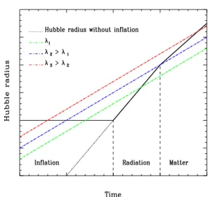
Let us now investigate how these scales behave in a typi-cal model of slow-roll inflation. For the purpose of illustra-tion, we only consider the scale factora(η)∝ |η|−1during inflation since we have seen before that any model of slow-roll inflation can be seen as a small deformation of the de Sitter space-time. One immediately obtains that the Hubble radius is constant during inflation while it varies as∝a2 du-ring the radiation era and as∝a3/2during the matter domi-nated era. Initially, the physical wavelengths are therefore smaller than the Hubble radius (in principle even smaller than the Planck length, see below) but because of the infla-tionary expansion of the background they become, at some point, larger than the Hubble radius. The time at which a Fourier mode exits the Hubble radius depends on the co-moving wavenumber of the corresponding mode. They will re-enter the Hubble radius later on, either during the radi-ation or matter dominated epochs because the Hubble ra-dius behave differently during those eras. It is worth no-ticing that, without a phase of inflation, the modes would have always been outside the Hubble radius. The fact that there is a regime where the modes are sub-Hubble is the-refore a specific feature of the inflationary background and plays a crucial role in our ability to fix well-defined initial conditions. The evolution of a Fourier mode is represented in Fig. 2.
It is also interesting to remark than the physical wave-lengths are always inside the horizon which they never exit. It is therefore mandatory to distinguish the horizon from the Hubble scale. In fact it is possible to prove that, as soon as a scale is inside the horizon, it will remain so for ever. This is simply due to the fact that the ratio of the horizon to the physical scale at timetis given by
dH
λ = k
2π
t0 ti
dτ a(τ)+
k
2π
t
t0
dτ
a(τ), (45)
where k is the co-moving wavenumber of the scale un-der consiun-deration. The first term is by assumption greater than one and the second one is positive, hence the above-mentioned statement
Figure 2. Evolution of the Hubble radius and of three physical wavelengths with different comoving wavenumbers during the inflationary phase and the subsequent radiation and matter domi-nated epochs. Without inflation, the wavelengths of the mode are super-Hubble initially whereas in the case where inflation takes place, they are sub-Hubble which permits to set up sensible initial conditions.
Looking at the equation of motion, one sees that,a pri-ori, the behavior of the solution is not controlled by the Hub-ble scale as often said in the literature (sometimes, it is also claimed that the horizon determines the qualitative behavior of the solutions!) but by the scaleℓU,i.e.by the shape of the effective potential. However, it turns out that, for slow-roll inflation (in fact for power-law inflation), the behaviors of
ℓUandℓHare similar and, therefore, the concepts of Hubble and potential scales can be used almost interchangeably in this situation. This is not the case in general. For instance, this is incorrect in a bouncing universe, see Ref. [16].
Let us now study in more details the shape of the effec-tive potential. The functionγ is a constant for power law scale factors and, as a consequence, the two types of per-turbations acquire the same potential during inflation, na-melyUS,T(η) ≃ η−
potential” and “outside the Hubble scale/below the poten-tial”. Let us notice that this is valid as long as the details of the reheating process only modify the shape of the poten-tial such that the modes of interest always remain below the potential during the transition from inflation to radiation.
The two previous regimes correspond to two types of solution. In the first regime, k2 ≫ U(η), and the mode function oscillates,
µS,T ≃A1(k)e− ikη+A
2(k)eikη. (46) On the contrary, when the potential dominates,k2≪U(η), the solutions are of the form
µS≃C1(k)a
√γ+C
2(k)a√γ
η dτ
(a2γ)(τ), (47) and possess a growing and a decaying modes. For gravi-tational waves, the solutions are the same except that one should takeγ= 1in the previous equation. It is interesting to notice that the previous solutions are general and do not depend on the specific form of the scale factor.
The only thing which remains to be discussed are the initial conditions,i.e. the choice of the coefficientsA1(k) andA2(k).
3.3
WKB approximation and the initial
con-ditions
It has been established before that the mode functionsµS andµT obey the equation of a parametric oscillator. This strongly suggests to use the WKB approximation to study the solutions of this equation [17]. For this purpose, let us define the WKB mode function,µWKB, by the following ex-pression
µWKB(k, η)≡
1
2ω(k, η)e
±i
η
ω(k, τ)dτ
. (48)
The mode functionµWKB represents the leading order term of a semi-classical expansion,i.e. it is only an approxima-tion to the actual soluapproxima-tion of Eq. (41). This can also be vi-ewed from the fact thatµWKB satisfies the following diffe-rential equation
µ′′
WKB(k, η)+
ω2(k, η)−Q(k, η)
µWKB(k, η) = 0, (49) which is not similar to Eq. (41). In the above formula, the quantityQ(k, η)is given by
Q(k, η)≡ 34(ω′)
2
ω2 −
ω′′
2ω, (50)
and only depends on the time dependent frequencyω(k, η). From Eqs. (41) and (49), it is clear that the mode func-tion µWKB(k, η) is a good approximation of the actual mode functionµ(k, η)if the following condition is satisfied:
|Q/ω2| ≪1. If, for simplicity, we only keep the first term in the expression givingQ(k, η), see Eq. (50), the above equa-tion can also be re-written under the more tradiequa-tional form
(dU/dη)/(k2−U)3/2 ≪ 1, which expresses the fact that the WKB approximation breaks down at the turning point and is valid when the potential does not vary too rapidly.
Let us now test this criterion for the two regimes des-cribed before. In the case of slow-roll inflation, we will see that the effective potential, either for density perturbations or gravitational waves, is of the formO(1)/η2. Therefore, on sub-Hubble scales, in the limit|η| →+∞, one hasω ≃k, which impliesQ≃0and therefore the|Q/ω2| ≪ 1is sa-tisfied. On the contrary, on super-Hubble scales,i.e., in the limit|η| →0, one has|Q/ω2|
S≃ |Q/ω 2|
T =O(1). Thus, the WKB approximation is not a good approximation in this regime.
The fact that the WKB approximation works in the limit
|η| → +∞allows us to fix well-motivated initial conditi-ons and is the reason why the inflationary mechanism for structure formation is so attractive. Indeed, within the fra-mework described before, the natural choice is to take the adiabatic vacuum as the initial state. Since, on sub-Hubble scales,ω(k)→k, Eq. (48) implies that this corresponds to coefficientsA1(k)andA2(k)in Eq. (46) such that
A1(k)∝
1
√
2k, A2(k) = 0. (51)
This completely fixes the initial conditions and allows us to calculate the power spectrum unambiguously.
Before turning to this calculation, let us quickly come back to the fact that the WKB approximation breaks down on super-Hubble scales. In fact, this problem bears a close resemblance with a situation discussed by atomic physicists at the time quantum mechanics was born. The subject deba-ted was the application of the WKB approximation to the motion in a central field of force and, more specifically, how the Balmer formula, for the energy levels of hydroge-nic atoms, can be recovered within the WKB approximation. The effective frequency for hydrogenic atoms is given by (obviously, in the atomic physics context, the wave equation is not a differential equation with respect to time but to the radial coordinater)
ω2(E, r) = 2m
2
E+Ze
2
r
−ℓ(ℓr+ 1)2 , (52)
whereZeis the (attractive) central charge andℓthe quantum number of angular momentum. The symbolE denotes the energy of the particle and is negative in the case of a bound state. Apart from the termZe2/rand up to the identification
r↔η, the effective frequency has exactly the same form as
approximation breaks down at smallr, for an effective fre-quency given by Eq. (52) and, in addition, he suggested a method to circumvent this difficulty. Recently, this method has been applied to the calculation of the cosmological per-turbations in Ref. [17]. This gives rise to a new method of approximation, different from the more traditional slow-roll approximation.
3.4
Simple calculation of the inflationary
power spectrum
Let us now evaluatek3P
ζ in a very simple way in order to understand why inflation leads to a scale invariant power spectrum. On super-Hubble scale, i.e. in region III in Fig. 3, the growing mode is given byµS ≃C1(k)a
√γ, see
Eq. (47). Inserting this expression into Eq. (42), one obtains
k3Pζ ∝k3|C1(k)|2. (53) The next step is to relate the constantC1(k)to the initial conditions,i.e. toA1(k). This can be done by writing the continuity of the mode functionµS at the time of potential crossing,i.e.at the time wherek2=U[η
j(k)]. In this case, one does not consider the details of region II in Fig. 3. One just matches by brute force the solutions of regions I and III. This gives
A1(k)e−ikηj =C1(k)(a√γ)(ηj). (54) In order to calculate the function ηj(k), one needs to as-sume something about the scale factor. Here, we consider power-law inflation with the scale factor: a(η) ∝ |η|1+β. In this case the effective potential is given byU(η) ∝η−2 (and in fact the equation of motion can be integrated exac-tly in terms of Bessel function) which amounts to take
ηj(k) ∝ k−1. Using also the fact thatγ is a constant for power-law inflation, the constant C1(k) can be easily de-termined from the above equation. Inserting the result into Eq. (53), one arrives at
k3P
ζ ∝k5+2β|A1(k)|2. (55) For the de Sitter case, β = −2, one obtains k3P
ζ ∝
k|A1(k)|2 ∝k0becauseA1(k)∝k−1/2,i.e. a scale inva-riant spectrum. The role of the adiabatic initial conditions, namely the fact that A1(k) ∝ k−1/2, is clearly crucial in order to obtain this result.
3.5
The slow-roll power spectra
We now evaluate the power spectra of density perturbations and gravitational waves at leading order in the slow-roll ap-proximation which gives a more accurate description than the previous back-to-the-envelop calculation. For this pur-pose, the details of region II, see Fig. 3, are now taken into account [21]. Instead of matching the mode function of re-gion I directly to the mode function of rere-gion III, we now carefully calculate the mode function in region II and per-form two matchings. The first one is between the modes function of regions I and II and the second one is between
the mode functions of regions II and III. In order to evaluate the mode function of region II only the calculation of the
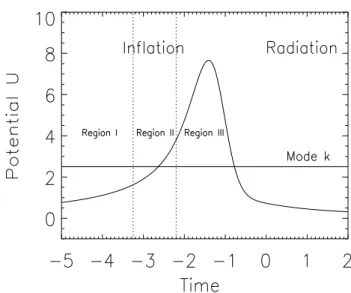
Figure 3. Sketch of the effective potential of Eqs. (39) and (40). During the inflationary phase the effective potential behaves as
U≃η−2while during the radiation dominated era it goes to zero.
A smooth transition between these two epochs has been assumed which does not take into account the details of the reheating (and preheating) process.
effective potentials is necessary. Using the definitions of the slow-roll parameters, one can show thatUS(η)can be re-written as
US(η)≡
(a√γ)′′
a√γ =a
2H2[2
−ǫ+ (ǫ−δ)(3−δ) +ξ].
(56) It has already been established that, at leading order,aH =
−(1 +ǫ)η−1. Therefore, one obtains that
US(η)≃
2 + 6ǫ−3δ
η2 , (57)
where one recalls that ǫ and δ should be considered as constant. As announced before, the potential has the form
US∝ O(1)η−
2. For gravitational waves, similar considera-tions lead toUT = (2 + 3ǫ)/η
2. Then, the crucial point is that the mode function can be found exactly. It is given in terms of Bessel functions
µII(η) =
kη[B1(k)Jν(kη) +B2J−ν(kη)], (58)
order in the slow-roll parameters, one obtains
k3Pζ = H 2
πǫm2 Pl
1−2 (C+ 1)ǫ−2C(ǫ−δ)
−2 (2ǫ−δ) ln k
k∗ , (59)
k3P
h =
16H2
πm2 Pl
1−2 (C+ 1)ǫ−2ǫln k
k∗
,(60)
where C is a numerical constant, C ≃ −0.73. Several remarks are in order at this point. Firstly, the amplitude of the scalar power spectrum depends on the Hubble para-meters during inflation and on the first slow parameter,i.e.
H2/(πǫm2Pl), while the amplitude of the tensor power spec-trum only depends on the scale of inflation,16H2/(πm2
Pl). The ratio of tensor over scalar is just given by16ǫ. This me-ans that the gravitational are always sub-dominant and that, when we measure the CMBR anisotropies, we essentially see the scalar modes. This is rather unfortunate because this implies that one cannot measure the energy scale of infla-tion since the amplitude of the scalar power spectrum also depends on the slow-roll parameterǫ. Only an independent measure of the gravitational waves contribution could allow us to break this degeneracy. Secondly, the spectral indices are given by
nS= 1−2ǫ1−ǫ2, nT =−2ǫ1. (61) As expected, the power spectra are always close to scale in-variance and the deviation from it is controlled by the mag-nitude of the two slow-roll parameters. Thirdly, at the next-to-leading order there is no running of the spectral indices sinceαS andαT are in fact second order in the slow-roll parameters.
4
Inflationary predictions
We now calculate the slow-roll parameters for typical mo-dels of inflation [22].
4.1
Large field models
These models typically appear in the chaotic inflationary scenario. The potential is simply given by a monomial of the inflaton field
V(φ0) = M 4 φ 0 mPl p . (62)
The calculation of the slow-roll parameters is then straight-forward if one uses Eqs. (29). One obtains
ǫ= p
2 16π φ 0 mPl −2
, δ= p(p−2) 16π φ 0 mPl −2 . (63)
To go further, it is convenient to express the slow-roll pa-rameters at Hubble crossing (remember that, at leading or-der, they must be considered as constant) or, equivalently, in terms of the number of e-foldsN∗ between the Hubble
radius exit and the end of inflation (not to be confused with the total number of e-folds). The number of e-folds N∗is given by the formula
N∗= ln
a end
a∗
≃ −m8π2 Pl
φend φ∗
dφ0V(φ0) dV
dφ0 −1
,
(64) whereφendis the value of the field at the end of inflation and
φ∗the value of the field at Hubble radius crossing. Inflation stops whenǫ= 1which, for chaotic inflation, is equivalent toϕend =mPlp/(4
√
π). The above integral can easily be performed and, using the explicit expression of φend, one arrives at
N∗=−
8π m2 Pl 1 p φend φ∗
dφ0φ0 ⇒
φ2 ∗ m2 Pl = p 4π
N∗+
p
4
.
(65) Inserting this formula into the equations giving the two slow-roll parameters, one obtains
ǫ1=
p
4(N∗+p/4)
, ǫ2=
1 (N∗+p/4)
. (66)
Therefore, in the space(ǫ1, ǫ2), a given model is represen-ted by the straight lineǫ1 = (p/4)ǫ2. However, in order to know precisely where a given model lies on the straight line requires the knowledge ofN∗which, in turns, depends on the parameters describing inflation like, for instance, the energy scale of inflation or the reheating temperature. We will come back to this point below.
4.2
Small field models
These models are characterized by potentials the shape of which, for small values of the inflaton field, can be approxi-mated by the following equation
V(φ0) = M 4 1− φ0 µ p . (67)
We assume that inflation takes place for values of the field smaller than the characteristic scaleµ,i.e.φ0≪µ. The two slow-roll parameters are given by
ǫ = p
2
16π
m Pl
µ
2 (φ 0/µ)
2(p−1)
[1−(φ0/µ) p
]2, (68)
δ = −ǫ−p(p8−π1)
m Pl
µ
2 (φ 0/µ)
p−2
[1−(φ0/µ) p
]. (69)
The value at which inflation stops is given by φend/µ ≃
16π/p21/(2p−2)
(µ/mPl) 1/(p−1)
. The next step is to ex-press everything in terms of N∗. Here, the modelp = 2
requires a special treatment and we start with this case. The integral giving the number of e-folds can be performed ex-plicitly
N∗= 4π
µ
mPl
2 φend/µ φ∗/µ
dx
1
x−x
from which one obtains
φ∗ µ ≃2
√ π µ
mPl
exp
−N∗
4π
m Pl
µ
2
. (71)
From the above equation, we immediately deduce that
ǫ1≃exp
−N∗
2π
m Pl
µ
2
≪1, ǫ2≃
1 2π
m Pl
µ
2
.
(72) We already see an important difference from the chaotic in-flation case. Sinceǫ1is tiny, the observational properties of the model will only be determined by the quantityǫ2which is aN∗independent quantity. Therefore, we do not need to calculate N∗in order to know where the model lies in the plane(ǫ1, ǫ2).
Let us now turn to the casesp >2. The method is exac-tly the same, the only change being that the integral giving
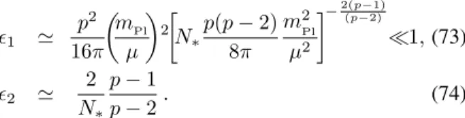
N∗ is now different but can still be performed analytically. After straightforward calculations, one arrives at
ǫ1 ≃
p2
16π
m Pl
µ
2N
∗
p(p−2) 8π
m2 Pl
µ2
−2(p(p−−2)1)
≪1,(73)
ǫ2 ≃
2
N∗ p−1
p−2. (74)
As for the case p = 2, the first slow-roll parameter is ne-gligible. However, the second slow-roll parameter is now a function ofN∗as for chaotic models.
4.3
The linear potential
The linear potential is simply given by the expression
V(φ0) = M 4
1−
φ0
µ , (75)
and we still assumeφ0 ≪ µ. Since we haveV′′ = 0, we deduce thatδ =−ǫorǫ1 =ǫ2/4which is consistent with the result already obtained for chaotic inflation. The first slow-roll parameter is independent of N∗ and is given by
ǫ1= 1/(16π)(mPl/µ) 2.
4.4
The exponential potential
This is an important potential since, in this case, everything can be done exactly. The potential is given by
V(φ0) = M 4exp
4√π mPl
√γ(φ
0−φi) , (76) The expression of the slow-roll parameters isǫ = δ = γ
which means ǫ2 = 0. The parameter γ can be written
γ = (2 +β)/(1 +β) whereβ is the power index of the exact scale factora(η)∝ |η|1+β. The caseβ =−2 corres-ponds to the exact de Sitter case for whichǫ = 0. In this case the amplitude of the slow-roll density power spectrum is not valid.
4.5
Hybrid inflation potentials
Hybrid inflation typically proceeds with two fields, the role of the second field being just to stop inflation. During the slow-roll phase, the potential has the following shape
V(φ0) = M
41 +φ0
µ
p
, (77)
withφ0 ≪ µ. Since another mechanism must be used in order to stop inflation, one cannot calculateφendin the sim-ple context considered here. However, if one assumes that
φ∗ ≪ µ, which is the case in concrete models of hybrid inflation, then one can deduce some general features of the model. In particular, one can calculate the ratio of the two slow-roll parameters
ǫ2
ǫ1
= 2−4(pp−1)
µ
φ∗
p
. (78)
This means that this type of models are such thatǫ2<0and
nS>1.
The results are summarized in Fig. 4 where the plan
(ǫ1, ǫ2)is represented.
Figure 4. The various models discussed in this article represen-ted in the plan(ǫ1, ǫ2). The dotted lines are the lines of constant spectral index. The full lines represent the location of the large field models. The small field models are concentrated along the
ǫ1 = 0, ǫ2 >0axis whereas the exponential models are along the
ǫ2= 0line. Hybrid models havenS>1andǫ2<0.
4.6
Comparison with the WMAP data
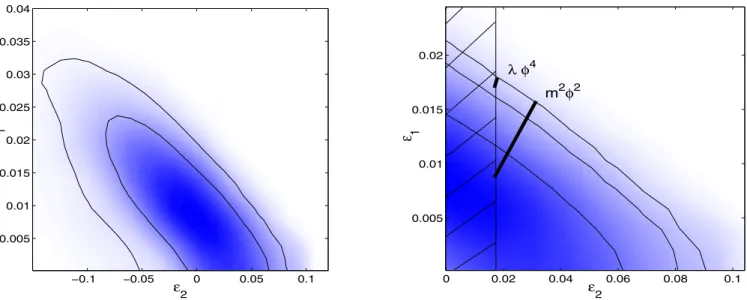
The aim of this section is to illustrate the fact that the high-accuracy data that are now at our disposal are now starting to discriminate among the various models of inflation pre-sented in the last sections. The constraints coming from the most recently released CMB data,i.e. the WMAP data [5], are represented in Fig. 5 following the analysis performed in Ref. [23]. Very roughly speaking, we have the constraints
As is clear from the previous analysis, except for a few models (like, for instance, the quadratic small field model or the exponential potential), the determination of the slow-roll parameters requires the calculation ofN∗which in turns de-mands the knowledge of the whole history of the universe.
Unfortunately all the details of this history are not known and hence there exits important uncertainties with regards to the precise value ofN∗in a particular model. This question has been recently re-analyzed in Ref. [24].
ε 2 ε 1
−0.1 −0.05 0 0.05 0.1
0.005 0.01 0.015 0.02 0.025 0.03 0.035 0.04
ε2
ε
10 0.02 0.04 0.06 0.08 0.1
0.005 0.01 0.015 0.02
m2φ2
λ φ4
Figure 5. Left panel: allowed region in the plan(ǫ1, ǫ2)coming from the recently released WMAP data as analyzed in Ref. [23]. Right panel: zoom of the left panel. The modelV(φ0)∝φ40is now under big observational pressure. These two figures are from Ref. [23].
Here, we just consider some examples to illustrate that, nevertheless, there exists now stringent constraints on the models. For instance, for the quadratic small field model,
|ǫ2| 0.1 implies thatµ/mPl 1 which is problematic for this model. For the exponential model,ǫ1 0.05 me-ans that β −2.053. In terms of the equation of state parameter, this means (since one must have β ≤ −2),
−1 p/ρ −0.966 during inflation. More importan-tly, the chaotic models are now severely constrained. In Refs. [23, 24], it has been shown that there is a limit onN∗
which implies thatǫ20.02(for chaotic models). This me-ans that the modelsV ∝φn
0, withn≥4are now under big pressure, as summarized in the right panel in Fig. 5. Other important conclusions can be obtained (in particular on the energy scale of inflation) and we refer the reader to Ref. [23] for more details.
5
Open issues for inflation and
con-clusions
Despite its impressive successes, inflation has problems. For instance, it would be clearly desirable to embed slow-roll in-flation into a realistic model of particle physics at high ener-gies (SUSY, SUGRA, string theory etc . . . ). Unfortunately, no obvious candidate has yet emerged (for a complete dis-cussion of the model building problem, see Ref. [25]).
Yet another open issue is the so-called trans-Planckian problem of inflation [26]. This is the fact that, at the be-ginning of inflation, the scales of astrophysical relevance to-day were smaller than the Planck length,i.e.where in a
re-gime where quantum field theory is expected to break down. Since the standard calculation of the power spectrum is ba-sed on quantum field theory, this questions the validity of its derivation. It is not easy to predict to which modificati-ons this could give rise since quantum gravity is not known. Fortunately, one can show that “reasonable” modifications of high-energy physics can leave an imprint on the obser-vables [27] like the CMBR multipole moments. Therefore, there is a hope to constrain the new physics with (future) high accuracy cosmological observations. This would be a concrete realization of the idea that cosmology can help us to understand high energy physics.
Acknowledgments
I would like to thank P. Peter and D. Schwarz for use-ful discussions and careuse-ful reading of the manuscript. I am especially indebted to S. Leach and A. Liddle for the autho-rization to use the figures of their article [23].
References
[1] A. Guth, Phys. Rev. D23, 347 (1981); A. Linde, Phys. Lett. B108, 389 (1982); A. Albrecht and P. J. Steinhardt, Phys. Rev. Lett.48, 1220 (1982); A. Linde, Phys. Lett. B129, 177 (1983).
[2] V. Mukhanov and G. Chibisov, JETP Lett.33, 532 (1981); Sov. Phys. JETP56, 258 (1982).
Rev. Lett.49, 1110 (1982); J. M. Bardeen, P. J. Steinhardt, and M. S. Turner, Phys. Rev. D28, 679 (1983).
[4] S. Leach, A. R. Liddle, J. Martin, and D. J. Schwarz, Phys. Rev. D66, 023515 (2002),astro-ph/0202094.
[5] C. L. Bennet at al., Astrophys. J. Suppl. 148, 1 (2003),
astro-ph/0302207.
[6] S. Dodelson,hep-ph/0309057.
[7] G. F. Smooth,et al., Astrophys. J.396, L1 (1992).
[8] G. F. R. Ellis and W. Stoeger, Class. Quant. Grav.5, 207 (1988).
[9] E. D. Stewart and D. H. Lyth, Phys. Lett. B302, 171 (1993).
[10] D. J. Schwarz, C. A. Terrero-Escalante, and A. A. Garcia, Phys. Lett. B517, 243 (2001),astro-ph/0106020.
[11] V. F. Mukhanov, H. A. Feldman, and R. H. Brandenberger, Phys. Rep.215, 203 (1992).
[12] J. A. Bardeen, Phys. Rev. D22, 1882 (1980).
[13] D. H. Lyth, Phys. Rev. D31, 1792 (1985).
[14] J. Martin and D. J. Schwarz, Phys. Rev. D57, 3302 (1998),
gr-qc/9704049.
[15] L. P. Grishchuk, Zh. Eksp. Teor. Fiz67, 825 (1974).
[16] J. Martin and P. Peter, Phys. Rev. D 68, 103517 (2003),
hep-th/0307077; J. Martin and P. Peter, Phys. Rev. Lett.
92, 061301 (2004),astro-ph/0312488.
[17] J. Martin and D. J. Schwarz, Phys. Rev. D67, 083512 (2003),
astro-ph/0210090.
[18] H. A. Kramers, Zeit. f. Physik39, 836 (1926).
[19] L. A. Young and G. E. Uhlenbeck, Phys. Rev. 36, 1158 (1930).
[20] R. E. Langer, Phys. Rev.51, 669 (1937).
[21] J. Martin and D. J. Schwarz, Phys. Rev. D 62, 103520 (2000), astro-ph/9911225; J. Martin, A. Riazu-elo, and D. J. Schwarz, Astrophys. J. 543, L99 (2000),
astro-ph/0006392.
[22] W. H. Kinney and K. T. Mahanthappa, Phys. Rev. D 53, 5455 (1996),hep-ph/9512241; S. Dodelson, W. H. Kin-ney, and E. W. Kolb, Phys. Rev. D 56, 3207 (1997),
astro-ph/9702166.
[23] S. Leach and A. Liddle,astro-ph/0306305.
[24] A. Liddle and S. Leach, Phys. Rev. D68, 103503 (2003),
astro-ph/0305263.
[25] D. Lyth and A. Riotto, Phys. Rept. 314, 1 (1999),
hep-ph/9807278.
[26] J. Martin and R. H. Brandenberger, Phys. Rev. D 63, 123501 (2001), hep-th/0005209; R. H. Brandenber-ger and J. Martin, Mod. Phys. Lett. A16, 999 (2001),
astro-ph/0005533.
[27] J. Martin and C. Ringeval, Phys. Rev. D69, 083515 (2004),