Indetermination Problem in the
Oaxaca-Blinder Decomposition: An
Application to the Gender Wage Gap in
Brazil
Luiz Guilherme Scorzafave
∗
, Elaine Toldo Pazello
†
Contents: 1. Introduction; 2. Identification: problem and solution; 3. An application to the Brazilian case; 4. Conclusion; A. Appendix.
Keywords:Oaxaca decomposition, woman, gender, wage, normalized regression. JEL Code:J16, J7, J31.
There are hundreds of works that implement the Oaxaca-Blinder decom-position. However, this decomposition is not invariant to the choice of reference group when dummy variables are used. This paper applies the solution proposed by Yun (005a,b) for this identification problem to Brazil-ian gender wage gap estimation. Our principal finding is the increasing difference in part-time work coefficients between men and women, which contributes to narrow the gender wage gap. Other studies in Brazil not using any correction of the identification problem have found different re-sults.
Há centenas de trabalhos que implementam a decomposição de Oaxaca-Blinder. Entretanto, esta decomposição não é invariante à escolha dos grupos de referência quando variáveis binárias são utilizadas como regressores. Este artigo aplica a solução proposta por Yun (005a,b) para este problema de iden-tificação à estimação do diferencial de salários por sexo no Brasil. A crescente diferença entre homens e mulheres no coeficiente da regressão associado ao tra-balho em meio período vem contribuindo para reduzir o diferencial de salários por sexo. Outros estudos já realizados no Brasil que não utilizaram qualquer correção do problema de identificação, encontraram resultados diferentes.
1. INTRODUCTION
The decomposition proposed by Oaxaca (1973) and Blinder (1973) has been applied in hundreds of studies around the world, including Brazil.1 In general, the methodology is applied to separate the wage differentials of distinct groups (men/women, white/non-white) in two components, one related to differences in observable characteristics of the two groups. For example, men could earn more because they have more experience or are more educated than women. Nevertheless, this part, called the “explained differential”, is responsible for only a fraction of the wage gap between the groups. The remaining gap, called the “unexplained differential”, is attributable to different returns to the characteristics between the two groups. For instance, men and women with the same level of education could receive different rewards.
Some authors attribute this unexplained gap to discrimination, but there is a controversy in the literature over whether this conclusion is valid. The argument against this idea is that one can only say that a differential is attributable to discrimination if the estimation has considered all variables that affect wages and are different between groups. Obviously, it is hard to believe that any regression specification can assure this.
Apart from this debate, the Oaxaca-Blinder decomposition can be used to assess the contribution of each variable to the explained and unexplained gap. However, Oaxaca and Ramson (1999) show that the differential share attributable to the model’s dummy variables depends on the choice of the reference group. On the other hand, the overall gap fraction due to “explained” and “unexplained” is not affected by this problem.
Additionally, Yun (005a,b) proposes a method to implement the Oaxaca-Blinder decomposition that solves this indetermination problem. He estimates “normalized” equations, imposing the restriction that the sum of the dummies’ coefficients have to be zero.
In the Brazilian case, there are no papers that consider this indetermination related to dummy vari-ables. So, the aim of this paper is to present the indetermination problem and the solution proposed by Yun (005b) and apply it to the Brazilian case. To do this, in the next section we show the indetermi-nation problem and the solution proposed by Yun (005b). Next, we apply this solution to three years in Brazil: 1988, 1996 and 2004. The choice of these years particularly allows a comparison with the results of Giuberti and Menezes-Filho (2005), who used 1988 and 1996 in their analysis.
2. IDENTIFICATION: PROBLEM AND SOLUTION
2.1. The problem
We present the identification problem in the Oaxaca-Blinder decomposition based on Oaxaca and Ramson (1999). Suppose that one estimates separate wage regressions for males and females. Sup-pose there is a set of dummy variables (d’s) and also L continuous variables (z’s) in the model, where
PJ
j=1dij = 1, and{i=m, f}. For instance, d could be region of residence. In country-regionBrazil,
J=5 (South, Southeast, North, Northeast, Midwest). Without loss of generality,di1will be the omitted
category. The separately estimated wage equations for typeiindividuals at the sample means are given by:
¯
yi= ˆαi0+
XJ
j=2
¯
dijˆγij+
XL
l=1z¯il
ˆ
δil=
XJ
j=1
¯
dijθˆij+
XL
l=1z¯il
ˆ
δil (1)
wherey¯iis the mean log wage,αˆi0is the estimated intercept,ˆγijis the estimated coefficient for the
dummy variabledij;ˆδilis a vector of estimated slope coefficients for the set of regressors comprising
the lth variable,zilis a vector of regressor means for the set of regressors comprising the lth variable,
ˆ
γij = ˆθij−θˆi1, and finally,αˆi0= ˆθi1.
Still following Oaxaca and Ramson (1999), the mean wage differences can be decomposed as follows:
¯
ym−y¯f =
= (ˆαm0−αˆf0) +
J
X
j=2
¯
df j(ˆγmj−γˆf j) + L
X
l=1
¯
zf∆ˆδl+ J
X
j=2
( ¯dmj−d¯f j)ˆγmj+ L
X
l=1
∆¯zlˆδml =
=
J
X
j=2
¯
df j(ˆθmj−θˆf j) + L
X
l=1
¯
zf l∆ˆδl+ J
X
j=1
( ¯dmj−d¯f j)ˆθmj+ L
X
l=1
∆¯zlδˆml (2)
where the last two terms in each equality measure the “endowment” effect, while the others capture the “discrimination” effect.
The first thing that Oaxaca and Ramson (1999, 156) indicate about this decomposition is that “the estimated overall discrimination and the estimated overall endowment effect are invariant to the choice of left-out reference group and the suppression of the constant term in the absence of a left-out refer-ence group.” The most important issue, however, is that the contribution of variable d to the discrim-ination effect is sensitive to the left-out reference group because the intercept varies with changes in that reference group. To see this, suppose that the last dummy variable has been chosen for the left-out reference group. In this case, the “discrimination” effect would bePJ−1
j=1df j( ˆφmj−φˆf j), where
ˆ
φij = ˆθij−θˆiJ.
Oaxaca and Ramson (1999) show that if there is only one set of dummy variables in the regression, this problem can be solved by incorporating (ˆαm0 −αˆf0) to the contribution of variable d to the
“discrimination” effect. However, this solution is not valid if there is more than one set of dummy variables in the estimated equation, a very common situation in the context of wage regressions.
2.2. The solution
Yun (005a) proposes a methodology to disentangle the identification problem, based on normalized regressions. The idea concerning normalized regressions is that if
“alternative reference groups yield different estimates of the (. . . ) coefficients effect for each individual variable, then it is natural to obtain estimates of the (. . . ) effect for every possible specification of the reference groups and take the average of the estimates of the (. . . ) effect with various reference groups as the ‘true’ contributions of individual variables to wage differentials.”Yun (005a, 766)
But Yun (005b) shows that one does not need to proceed in this cumbersome way. It is possible to implement the method by estimating only one equation. To illustrate the method, we follow Yun (005b) and suppose that we have a set of dummy variables (d’s) and also L continuous variables (z’s) in the model as before and, additionally, another set of dummy variables (q’s). To simplify the presentation, we ignore the subscript i in this section.
y=α+
XJ
j=2djγj+
XK
k=2qkλk
+XL
l=1zlδl+e (3)
This equation is called the “usual regression” and he proposes an alternative specification that does not omit the reference group:
y=α∗+
XJ
j=1djγ
∗
j +
XK
k=1qkλ
∗
k
+XL
l=1zlδl+e (4)
the intercept changes fromα+γ1toα+γr. But taking on this averaging approach implies imposing
thatPJ
j=1γj∗ = 0and
PK
k=1λ∗k = 0, as Suits (1984) states. Particularly, “since these restrictions do
not have unique solutions,” he specifies the coefficients of the normalized regression asγ∗
j =γj+mγ
andλ∗
j =λj+mλ, and refines the problem of deriving the normalized regressions as finding values of
mγandmλ. It turns out that their values aremγ =−PJj=1γj/J andmλ =−PKk=1λk/K, where
γ1=λ1= 0Yun (005b, 3). Considering this, Yun (005b) proposes the “normalized equation”:
y= (α+γ+λ) +
XJ
j=1dj(γj−γ) +
XK
k=1qk(λk−
¯
λ)
+XL
l=1zlδl+e (5)
whereγ=PJ
j=1γj/J,¯λ=
PK
k=1λk/Kandγ1=λ1= 0.
If we estimate equation (4) for men and women separately, we can implement the Oaxaca decom-position of the wage equation that is invariant to the choice of the omitted category in the dummy variables.
3. AN APPLICATION TO THE BRAZILIAN CASE
In this section we apply the solution provided by Yun (005b) to solve the identification problem. Initially, we obtain the normalized regressions and after that we apply the Oaxaca decomposition. We use data from the Brazilian National Household Survey (Pesquisa Nacional de Amostra por Domicilios – PNAD), conducted annually by the Brazilian Institute of Geography and Statistics (Instituto Brasileiro de Geografia e Estatística – IBGE, the Brazilian census bureau), for three years, 1988, 1996 and 2004.
The sample is composed of individuals between the ages of 25 and 54 living in urban areas who have positive job earnings. The choice of this age range is justified because it is the most important in terms of participation in the labor market. The exclusion of residents of rural areas is due to the change in the PNAD sample in 2004, which began to incorporate the rural area of the North region. Therefore, if we included these individuals, the comparison of the results among the three years would be impaired. Finally, since we work only with individuals with positive job earnings (i.e., we exclude labor that is not remunerated), we avoid the problem of harmonization of the PNADs starting in 1992 with previous surveys.2
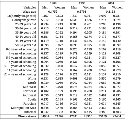
Table 1 presents the description of the data. The data on labor income refer to the hourly wage, measured in Reais of January 2002, deflated according to the index proposed in Corseuil and Foguel (2002).
The first thing that is interesting to note is that the gender wage gap narrowed in Brazil, from 0.475 in 1988 to 0.216 in 2004. In other words, in 1988, men earned 47.5% higher wages than women, but in 2004 this difference had fallen to 21.6%. In terms of education, there was a substantial improvement in the Brazilian situation over that interval. For instance, the proportion of men with 11 years of schooling increased 11.4 percentage points between 1988 and 2004. Despite this fact, women continue to be more educated than men. In 2004, 21% of women had 12 or more years of schooling, while only 14% of men had attained this level. In turn, the age profile of men and women is quite similar. With regard to the region of residence, the data show a concentration of Brazilian workers in the Southeast, Northeast and South regions, and remarkably, a falling proportion of workers living in metropolitan areas. However, the most interesting fact is the increasing proportion of men working in part-time activities along with a decrease in this number among women. Despite this, 14.5% of the female workers were in part time activities, while there were only 3.4% of men in this situation in 2004. Concerning informality, the gap
2In 1992, the PNAD began to classify workers in production for their own consumption, construction for their own use and those
Table 1 –Proportion of workers in each group, wages and wage gap.
1988 1996 2004
Variables Men Women Men Women Men Women Wage gap 0.4752 0.2791 0.2158 Ln(hourly wage rate) 1.167 0.692 1.230 0.951 0.997 0.781
Hourly wage rate 5.917 3.790 6.025 4.626 4.714 3.574 25-29 years old 0.234 0.243 0.203 0.201 0.203 0.198 30-34 years old 0.215 0.224 0.214 0.221 0.193 0.196 35-39 years old 0.186 0.192 0.194 0.205 0.184 0.191 40-44 years old 0.151 0.154 0.168 0.174 0.172 0.177 45-49 years old 0.119 0.110 0.131 0.125 0.142 0.140 50-54 years old 0.095 0.077 0.090 0.075 0.106 0.097 0-3 years of schooling 0.270 0.248 0.220 0.179 0.162 0.119 4 years of schooling 0.237 0.199 0.179 0.159 0.129 0.108 5-7 years of schooling 0.102 0.084 0.143 0.121 0.154 0.127 8 years of schooling 0.094 0.080 0.121 0.106 0.121 0.106 9-10 years of schooling 0.037 0.038 0.047 0.045 0.055 0.051 11 years of schooling 0.128 0.165 0.167 0.208 0.242 0.279 12 + years of schooling 0.128 0.176 0.121 0.181 0.137 0.210 White 0.631 0.615 0.608 0.618 0.550 0.579 North 0.039 0.039 0.047 0.044 0.062 0.055 Mid-West 0.071 0.070 0.075 0.074 0.077 0.077 Northeast 0.182 0.199 0.196 0.208 0.211 0.206 Southeast 0.556 0.543 0.519 0.512 0.484 0.491 South 0.153 0.148 0.163 0.162 0.160 0.165 Part-time 0.017 0.156 0.031 0.151 0.034 0.145 Metropolitan Area 0.448 0.480 0.388 0.413 0.363 0.387 Informal 0.247 0.362 0.368 0.415 0.380 0.403 Observations 34938 21764 42041 28910 55159 42434
between men and women fell considerably in the period, from 12 percentage points to 2 points in favor of women. The main cause of this decrease was the huge informality growth among men between 1988 and 1996.
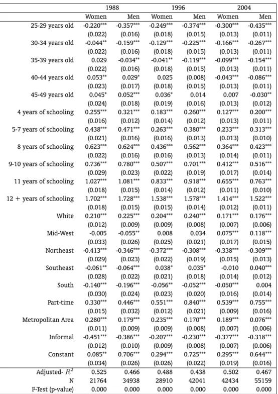
After this short discussion of the descriptive statistics, we are able to evaluate the results of the methodology adopted by the paper. First we analyze the regression estimate results (eq.2), which are in the appendix (Table 6). The dependent variable is the logarithm of hourly wage and the independent variables are dummies for age (25-29, 30-34, 35-39, 40-44, 45-49, 50-54), schooling (0-3, 4, 5-7, 8, 9-10, 11, 12 years or more), race (white, non-white), region (North, Northeast, Southeast, South, Midwest), part-time (working less than 20 hours per week), informal (do not contribute to social security system3) and metropolitan area.
In all years, the coefficients’ signs are aligned as expected. In terms of age, the coefficients show a positive relationship between wage and age for ages between 25 and 39. For other ages, there is no regular relation. The results also indicate that the higher the educational level, the greater the wage. It is interesting to observe the sheepskin effect in the educational estimates, although the returns of education show a decrease between 1988 and 2004. The white coefficient has the sign normally obtained, independent of gender, that is, white workers earn more than comparable non-white workers.
3A word of caution is necessary here, because in 1988, by our definition of informality, some public sector workers have been
However, this difference is smaller in 2004 than in previous years. The regional dummies are different for the periods. In the case of the Midwest, the wages were smaller than in the North region (reference group) in 1988 and became greater in 2004. Those in the Northeast are systematically lower than in the North for all years. In the other regions the wage differential, which favored the North in 1988, ceased existing (South) or reversed (Southeast) in the other periods. The part-time coefficient has a positive sign for both women and men, with a larger magnitude for men. There is a significant increase in the coefficient in 1996, doubling in the case of men. In 2004, the coefficient falls, but is still higher than in 1988. The metropolitan coefficient indicates that individuals living in metropolitan areas earn higher wages than others. However, the differential declines over the period studied. Finally, workers in the informal sector earn lower wages than other workers in all the years analyzed, occurring a sharp fall in 1996 relative to the other years.
The appendix also contains the estimation results of equation (4) for 1988 (Table 7), 1996 (Table 8) and 2004 (Table 9). We can see that the sum of the coefficients of each category is zero, as required to apply the Oaxaca decomposition without the indetermination problem.
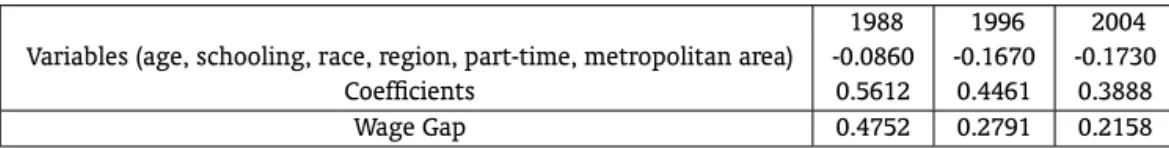
The Oaxaca decomposition technique permits identifying the factors that explain the wage differ-ential between men and women, dividing them into two types: a part attributed to the observable characteristics and another part attributed to the “market return” to these characteristics. The second part could be attributed to “discrimination”, because men and women receive different prices for their characteristics. Table 2 shows the evolution of the gender wage gap and the decomposition analysis.
Table 2 –Evolution of wage gender gap and of decomposition analysis
1988 1996 2004 Variables (age, schooling, race, region, part-time, metropolitan area) -0.0860 -0.1670 -0.1730
Coefficients 0.5612 0.4461 0.3888 Wage Gap 0.4752 0.2791 0.2158
As argued above, the data show a significant decrease in the gender-wage gap between 1988 and 2004. In 1988, men’s wages were 47.5% higher than women’s, but in 2004 this advantage dropped to 21.6%. The characteristics contribute to reduce the gap and the coefficients to raise the gap. If we were sure that the model was including all characteristics that explain the gap, the evidence would indicate the existence of discrimination favoring men. However, it is important to say that the main source of the fall in the gap between the years was the decline of the ’discrimination’ term. The next three tables show the gender wage gap decomposition using the traditional and the normalized equation, respectively, in 1988, 1996 and 2004.
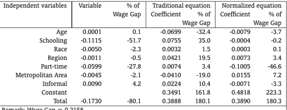
Columns 1 and 2 show the variables’ contribution to the wage gap (which is the same in the tradi-tional and normalized regressions). Two of the most important variables are schooling and the part-time dummy. These variables contribute to diminish the wage differential. The estimates (in the appendix) show a positive relation between these variables and wages. So, since women are on average more educated than men and they are the majority in part-time occupations, these variables contribute to reduce the gender wage gap. On the other hand, the higher informality among women contributes to explain 11% of the gender wage gap in 1988. The contribution of the other variables is very small.
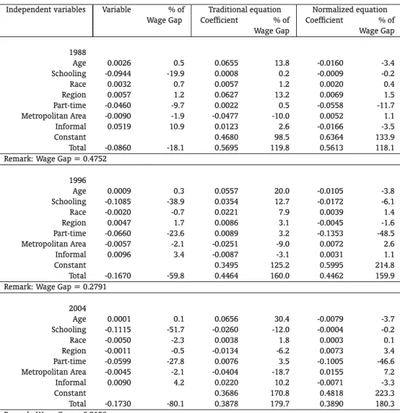
The coefficients’ effects are very different when we use the traditional instead of the normalized equation.4 This highlights the importance of the methodology applied here. For instance, the results using the traditional equation indicate that while age contributes to diminish the gap, schooling con-tributes to raise it. On the other hand, when the normalized regression is used, the effects of the
4Table 10 of the appendix presents the results of the decomposition altering the omitted group of the schooling, age and region
Table 3 –Gender wage gap decomposition – 1988
Independent variables Variable % of Traditional equation Normalized equation Wage Gap Coefficient % of Coefficient % of Wage Gap Wage Gap Age 0.0026 0.5 -0.0713 -15.0 -0.0160 -3.4 Schooling -0.0944 -19.9 0.0310 6.5 -0.0009 -0.2 Race 0.0032 0.7 0.0094 2.0 0.0020 0.4 Region 0.0057 1.2 -0.0017 -0.4 0.0069 1.5 Part-time -0.0460 -9.7 0.0020 0.4 -0.0558 -11.7 Metropolitan Area -0.0090 -1.9 -0.0451 -9.5 0.0052 1.1 Informal 0.0519 10.9 0.0162 3.4 -0.0166 -3.5 Constant 0.6207 130.6 0.6364 133.9 Total -0.0860 -18.1 0.5612 118.1 0.5613 118.1 Remark: Wage Gap = 0.4752
Table 4 –Gender wage gap decomposition - 1996
Independent variables Variable % of Traditional equation Normalized equation Wage Gap Coefficient % of Coefficient % of Wage Gap Wage Gap Age 0.0009 0.3 -0.0695 -24.9 -0.0105 -3.8 Schooling -0.1085 -38.9 0.0740 26.5 -0.0172 -6.1 Race -0.0020 -0.7 0.0217 7.8 0.0039 1.4 Region 0.0047 1.7 0.0141 5.0 -0.0045 -1.6 Part-time -0.0660 -23.6 0.0089 3.2 -0.1353 -48.5 Metropolitan Area -0.0057 -2.1 -0.0251 -9.0 0.0072 2.6 Informal 0.0096 3.4 -0.0086 -3.1 0.0031 1.1 Constant 0.4306 154.3 0.5995 214.8 Total -0.1670 -59.8 0.4461 159.8 0.4462 159.9 Remark: Wage Gap = 0.2791
Table 5 –Gender wage gap decomposition – 2004
schooling and age coefficients turn out to act in the same direction (to reduce the gap) and also lose significance. However, the main change is that the part-time dummy gains relevance in this decompo-sition. In 1988, the return of this characteristic contributes to reduce the total differential by 11.7% and in 2004 by 46.6%, that is, women’s comparative advantage in these occupations could possibly explain the falling wage gap between 1988 and 2004.
4. CONCLUSION
There are hundreds of works all over the world that implement the Oaxaca-Blinder decomposition. However, most of these works are plagued by the identification problem when a set of dummy variables is used, as Oaxaca and Ramson (1999) show.
In this paper, we applied the solution proposed by Yun (005a,b) to the Brazilian gender-wage gap estimation. Our first finding is that the gender gap has been narrowing in Brazil since 1988. The results also show that as women are more educated and more engaged in part time activities than men, these factors contribute to reduce the gender gap. On the other hand, the difference in the constant term between men and women explains the entire wage differential. However, the increasing difference in the part-time coefficients between men and women is contributing to alleviate this situation and can also be indicated as responsible for the narrowing gender wage gap in Brazil since 1988.
Giuberti and Menezes-Filho (2005), who do not use any correction to the identification problem, conclude that different returns related to age are important to explain the wage gap and the part-time dummy is not important. However, as demonstrated in this work, these results arise basically from the choice of the omitted categories of the qualitative variables incorporated in the regression model. The application of the methodology of Yun (005a), which resolves the indetermination problem, as said before, highlights the importance of the part-time variable in the decline in the gender wage gap in Brazil over the past 20 years.
Bibliography
Blinder, A. S. (1973). Wage discrimination: Reduced form and structural estimates.The Journal of Human Resources, 8(7):436–455.
Corseuil, C. & Foguel, M. (2002). Uma sugestão de deflatores para rendas obtidas a partir de algumas pesquisas domiciliares do ibge.Texto para Discussão IPEA, 9(897).
Giuberti, A. & Menezes-Filho, N. (2005). Discriminação dos rendimentos por gênero: uma comparação entre o Brasil e os Estados Unidos. Economia Aplicada, 9(3):369–383.
Kassouf, A. L. (1998). Wage gender discrimination and segmentation in the Brazilian labor market.
Brazilian Journal of Applied Economics, 2(2):243–269.
Lovell, P. A. & Wood, C. H. (1998). Skin color, racial identity and life chances in Brazil. Latin American Perspectives, 25(3):90–109.
Oaxaca, R. (1973). Male-female wage differentials in urban labor markets.International Economic Review, 14:693–709.
Oaxaca, R. & Ramson, M. (1999). Identification in detailed wage decompositions. Review of Economics and Statistics, 81(1):154–157.
Suits, D. (1984). Dummy variables: Mechanics v. interpretation. Review of Economics and Statistics, 66(1):177–180.
Yun, M. (2005a). A simple solution to the identification problem in detailed wage decompositions.
Economic Inquiry, 43(4):766–772.
Yun, M. (2005b). Normalized equation and decomposition analysis: computation and inference. IZA Discussion Paper, Institute for the Study of Labor, 9(1822).
Table 6 –Estimated Coefficients - Wage Equation (2) - Men and Women - 1988, 1996 and 2004
1988 1996 2004
Table 7 –Estimated Coefficients - Wage Equation (4) - Men and Women - 1988
Women Men 25-29 years old -0,197*** -0,279*** (0,011) (0,008) 30-34 years old -0,021** -0,081***
(0,011) (0,008) 35-39 years old 0,051*** 0,044***
(0,011) (0,009) 40-44 years old 0,076*** 0,107***
(0,012) (0,01) 45-49 years old 0,068*** 0,130***
(0,014) (0,011) 50-54 years old 0,023 0,078***
(0,016) (0,012) 0-3 years of schooling -0,683*** -0,715***
(0,012) (0,009) 4 years of schooling -0,428*** -0,394***
(0,012) (0,009) 5-7 years of schooling -0,245*** -0,244***
(0,016) (0,012) 8 years of schooling -0,060*** -0,091***
(0,017) (0,012) 9-10 years of schooling 0,053** 0,065***
(0,023) (0,019) 11 years of schooling 0,344*** 0,366***
(0,013) (0,011) 12 + years of schooling 1,019*** 1,013***
(0,013) (0,011) White 0,105*** 0,113***
(0,006) (0,005) Non-white -0,105*** -0,113***
(0,006) (0,005) North 0,124*** 0,132***
(0,022) (0,017) Mid-West 0,118*** 0,077***
(0,017) (0,013) Northeast -0,289*** -0,214***
(0,012) (0,01) Southeast 0,063*** 0,068***
(0,01) (0,008) South -0,016 -0,064***
(0,013) (0,011) Part-time 0,165*** 0,223***
(0,007) (0,016) Full-time -0,165*** -0,223***
(0,007) (0,016) Metropolitan Area 0,140*** 0,090***
(0,005) (0,004) Non-Metropolitan Area -0,140*** -0,090***
(0,005) (0,004) Informal -0,226*** -0,193***
(0,006) (0,005) Formal 0,226*** 0,193***
(0,006) (0,005) Constant 0,806*** 1,443***
(0,01) (0,017) Adjusted-R2 0.525 0.466
N 21764 34938 F-Test (p-value) 0.000 0.000
Table 8 –Estimated Coefficients - Wage Equation (4) - Men and Women - 1996
Women Men 25-29 years old -0,189*** -0.138*** (0,009) (0.007) 30-34 years old -0,069*** -0.016**
(0,009) (0.007) 35-39 years old 0,019** 0.069***
(0,009) (0.007) 40-44 years old 0,084*** 0.161***
(0,009) (0.008) 45-49 years old 0,095*** 0.171***
(0,011) (0.008) 50-54 years old 0,060*** -0.247***
(0,013) (0.005) 0-3 years of schooling -0,537*** -0.573***
(0,01) (0.006) 4 years of schooling -0,354*** -0.297***
(0,01) (0.006) 5-7 years of schooling -0,274*** -0.329***
(0,011) (0.007) 8 years of schooling -0,101*** -0.070***
(0,012) (0.008) 9-10 years of schooling -0,030* -0.057***
(0,017) (0.011) 11 years of schooling 0,296*** 0.313***
(0,009) (0.007) 12 + years of schooling 1,001*** 1.013***
(0,01) (0.009) White 0,102*** 0.118***
(0,005) (0.003) Non-white -0,102*** -0.118***
(0,005) (0.003) North 0,077*** 0.103***
(0,017) (0.012) Mid-West 0,084*** 0.075***
(0,013) (0.009) Northeast -0,295*** -0.257***
(0,009) (0.006) Southeast 0,114*** 0.093***
(0,008) (0.005) South 0,020* -0.013* (0,01) (0.007) Part-time 0,276*** 0.356***
(0,006) (0.007) Full-time -0,276*** -0.356***
(0,006) (0.007) Metropolitan Area 0,117*** 0.118***
(0,004) (0.003) Non-Metropolitan Area -0,117*** -0.118***
(0,004) (0.003) Informal -0,103*** -0.166***
(0,005) (0.003) Formal 0,103*** 0.166***
(0,005) (0.003) Constant 1,087*** 1.476***
(0,008) (0.008) Adjusted-R2 0.488 0.438
N 28910 42041 F-Test (p-value) 0.000 0.000
Table 9 –Estimated Coefficients - Wage Equation (4) - Men and Women - 2004
Women Men 25-29 years old -0.200*** -0.273*** (0.007) (0.006) 30-34 years old -0.066*** -0.105***
(0.007) (0.006) 35-39 years old 0.001 0.008
(0.007) (0.006) 40-44 years old 0.057*** 0.076***
(0.007) (0.006) 45-49 years old 0.107*** 0.132***
(0.008) (0.007) 50-54 years old 0.100*** 0.162***
(0.009) (0.008) 0-3 years of schooling -0.458*** -0.534***
(0.009) (0.007) 4 years of schooling -0.331*** -0.334***
(0.009) (0.008) 5-7 years of schooling -0.225*** -0.221***
(0.008) (0.007) 8 years of schooling -0.094*** -0.111***
(0.009) (0.008) 9-10 years of schooling -0.046*** -0.018* (0.012) (0.011) 11 years of schooling 0.197*** 0.229***
(0.006) (0.006) 12 + years of schooling 0.956*** 0.988***
(0.007) (0.008) White 0.085*** 0.088***
(0.004) (0.003) Non-white -0.085*** -0.088***
(0.004) (0.003) North 0.064*** 0.029***
(0.011) (0.009) Mid-West 0.140*** 0.148***
(0.010) (0.009) Northeast -0.273*** -0.280***
(0.007) (0.006) Southeast 0.055*** 0.070***
(0.006) (0.005) South 0.014* 0.033***
(0.008) (0.007) Part-time 0.269*** 0.377***
(0.005) (0.008) Full-time -0.269*** -0.377***
(0.005) (0.008) Metropolitan Area 0.094*** 0.038***
(0.003) (0.003) Non-Metropolitan Area -0.094*** -0.038***
(0.003) (0.003) Informal -0.188*** -0.159***
(0.004) (0.003) Formal 0.188*** 0.159***
(0.004) (0.003) Constant 0.849*** 1.331***
(0.006) (0.008) Adjusted-R2 0.502 0.467
N 42434 55159 F-Test (p-value) 0.000 0.000
Table 10 –Gender wage gap decomposition - 1988, 1996 and 2004
Independent variables Variable % of Traditional equation Normalized equation Wage Gap Coefficient % of Coefficient % of
Wage Gap Wage Gap 1988
Age 0.0026 0.5 0.0655 13.8 -0.0160 -3.4 Schooling -0.0944 -19.9 0.0008 0.2 -0.0009 -0.2 Race 0.0032 0.7 0.0057 1.2 0.0020 0.4 Region 0.0057 1.2 0.0627 13.2 0.0069 1.5 Part-time -0.0460 -9.7 0.0022 0.5 -0.0558 -11.7 Metropolitan Area -0.0090 -1.9 -0.0477 -10.0 0.0052 1.1 Informal 0.0519 10.9 0.0123 2.6 -0.0166 -3.5 Constant 0.4680 98.5 0.6364 133.9 Total -0.0860 -18.1 0.5695 119.8 0.5613 118.1 Remark: Wage Gap = 0.4752
1996
Age 0.0009 0.3 0.0557 20.0 -0.0105 -3.8 Schooling -0.1085 -38.9 0.0354 12.7 -0.0172 -6.1 Race -0.0020 -0.7 0.0221 7.9 0.0039 1.4 Region 0.0047 1.7 0.0086 3.1 -0.0045 -1.6 Part-time -0.0660 -23.6 0.0089 3.2 -0.1353 -48.5 Metropolitan Area -0.0057 -2.1 -0.0251 -9.0 0.0072 2.6 Informal 0.0096 3.4 -0.0087 -3.1 0.0031 1.1 Constant 0.3495 125.2 0.5995 214.8 Total -0.1670 -59.8 0.4464 160.0 0.4462 159.9 Remark: Wage Gap = 0.2791
2004