The Existence, Uniqueness and Error Bounds of Approximation Splines Interpolation for Solving Second-Order Initial Value Problems

(1)

ISSN 1549-3644

Corresponding Author: Abbas Y. Al Bayati, Department Mathematics, Mosul University, Mosul, Iraq

The Existence, Uniqueness and Error Bounds of Approximation Splines

Interpolation for Solving Second-Order Initial Value Problems

1

Abbas Y. Al Bayati,

2

Rostam K. Saeed and

3

Faraidun K. Hama-Salh

1

Department Mathematics, Mosul University, Mosul, Iraq

2

Department of Mathematics, Salahaddin University, Erbil, Iraq

3

Department of Mathematics, Sulaimani University, Sulaimani, Iraq

Abstract: Problem statement: The lacunary interpolation problem, which we had investigated in this study, consisted in finding the six degree spline S(x) of deficiency four, interpolating data given on the function value and third and fifth order in the interval [0,1]. Also, an extra initial condition was prescribed on the first derivative. Other purpose of this construction was to solve the second order differential equations by two examples showed that the spline function being interpolated very well. The convergence analysis and the stability of the approximation solution were investigated and compared with the exact solution to demonstrate the prescribed lacunary spline (0, 3, 5) function interpolation. Approach: An approximation solution with spline interpolation functions of degree six and deficiency four was derived for solving initial value problems, with prescribed nonlinear endpoint conditions. Under suitable assumptions, the existences; uniqueness and the error bounds of the spline (0, 3, 5) function had been investigated; also the upper bounds of errors were obtained. Results: Numerical examples, showed that the presented spline function proved their effectiveness in solving the second order initial value problems. Also, we noted that, the better error bounds were obtained for a small step size h. Conclusion: In this study we treated for a first time a lacunary data (0,3,5) by constructing spline function of degree six which interpolated the lacunary data (0,3,5) and the constructed spline function applied to solve the second order initial value problems.

Key words: Existence and uniqueness, spline function, mathematical model, 2nd order differential equations

INTRODUCTION

The initial value problems play an important role in mathematical physics, because many problems in science and technology are formulated mathematically in boundary value problems as in heat transfer and deflection in cables.

Several numerical methods have been investigated for calculating the solutions of such problems. Among these, finite difference techniques and the shooting method play an important role. These methods provide the value of the unknown of some grid knots. If we want the solution at the points, there is a need of interpolating these values. Also, spline functions of Hermite types has been used by many authors for solving these problems[6,9-12].

The literature on the numerical solutions of initial value problems by using lacunary spline functions is not too much. Gyovari[2] solved Cauchy problem by sing modified lacunary spline function which interpolating the lacunary data (0, 2, 3) Saxena[7]. used

deficient lacunary spline for solving Cauchy problem also. Saxena and Venturino[8] used two-point boundary value problem by using lacunary spline function which interpolates the lacunary data (0, 2). Ahmed et al.[1] found the approximation solution of the fourth order lacunary spline functions.

In this study, we try to solve the initial value problem:

0 1 1 2

y′′=f (x, y, y ) , y(x )′ =y , y (x )′ =y′ (1)

by using that n 1 2

f∈C−([0,1] R )× , n≥2and that it

satisfies the Lipschitz continuous:

{

}

(q)

1 1 2 2 1 2 1 2

f (x, y , y ) f (x, y , y )′ − ′ ≤L y −y + y′−y′

q = 0,1, …, n-1

(2)

This study is organized as follows: First consider the spline function of degree six is presented which interpolates the lacunary data (0, 3, 5). Some theoretical results about existence and uniqueness of the spline function of degree six are introduced and also convergence analysis is studied. To demonstrate the convergence of the prescribed lacunary spline function, numerical examples presented, finally, we prescribe the conclusion and discussion of the result.

MATERIALS AND METHODS

Descriptions of the method: We present for the first time according to our knowledge a six degree spline (0, 3, 5) interpolation for one dimensional and given sufficiently smooth function f(x) defined on i = [0,1] and ∆n: 0=x0< <x1 x2<....<xn=1.

Denote the uniform partition of I with knots xi = ih,

where i = 0, 1, 2, …, n-1. We denote by 5 n,6

S the class of six degree splines S(x) such that:

3

2 0

0 0 0 0 0 0, 2 0

5

4 0 (5) 6

0 0,4 0 0 0,6

(x x )

s (x) y (x x )y (x x ) a y

6

(x x )

(x x ) a y (x x ) a

120

−

′ ′′′

= + − + − + +

−

− + + −

(2)

on the interval [x0, x1] where a0,j, j = 2,4,6 are

unknowns to be determined[4,5].

Let us examine now intervals [xi, xi+1], i = 1,2,…,

n-2. By taking into account the interpolating conditions, we can write the expression, for Si(x) in the following

form:

3

2 i

i i i i,1 i i, 2 i

5

4 i (5) 6

i i,4 i i i,6

(x x )

s (x) y (x x )a (x x ) a y

6

(x x )

(x x ) a y (x x ) a

120

− _′′′

= + − + − + +

−

− + + −

(3)

where, a ,ii, j =1(1)(n 1) , j 1, 2, 4, 6− = are unknowns we need to determine it.

On the last interval [xn-1, xn] we define Sn(x) as

follows:

2 n n 1 n 1 n 1,1 n 1 n 1,2

3

4 n 1

n 1 n 1 n 1,4 5

(5) 6

n 1

n 1 n 1 n 1,6

s (x) y (x x )a (x x ) a

(x x )

y (x x ) a

6

(x x )

y (x x ) a

120

− − − − −

−

− − −

−

− − −

= + − + −

− _′′′

+ + −

−

+ + −

(4)

where, an-1,j, j = 1,2,4,6 are unknowns to be

determined.

The existence and uniqueness theorem for spline function of degree six which interpolate the lacunary data (0, 3, 5) are presented and examined.

Theorem 1: Existence and uniqueness: Given the real numbers y(xi), y(3)(xi) and y(5)(xi) for i = 0, 1, 2, …, n,

then there exist a unique spline of degree six as given in the Eq. 2-4 such that:

i i

(r ) (r)

i i

0 0

S(x ) y(x )

S (x ) y (x ), r 3,5

for i 0, 1,..., n and

S (x ) y (x )

= 



= = 

=

  

′ = ′ 

(5)

Proof: Let as define a spline function S(x) as follows:

0 0 1

i i i 1

n n 1 n

S (x) when x [x , x ]

S(x) S (x) when x [x , x ]; i 0,1,..., n 2

S (x) when x [x , x ]

+

− ∈

 

= ∈ = −

 _∈



where the coefficients of these polynomials are to be determined by the following conditions:

i i 1 i 1 i 1 i 1

(r ) (r )

i i 1 i 1 i 1 i 1

' '

i i 1 i 1 i 1

S (x ) S (x ) y

S (x ) S (x ) y , r 3,5 ; i 0,1,..., n 2

S (x ) S (x )

+ + + +

+ + +

= = 



= = =  = −



= 

(6)

and

(r ) (r ) n 1 n n n 1 n n

S−(x )=y , S− (x )=y ; r=3,5 (7)

To find uniquely the coefficients in S0(x) of Eq. 2

by using the condition (3.2) where i = 0, we obtain the following:

2 4 6

0.2 0.4 0.6 1 0 0

3 5

(3) (5)

0 0

h a h a h a y y hy

h h

y y

6 120

′

+ + = − − −

−

2

3 (3) (3) (5)

0.4 0,6 1 0 0 0

h

24ha 120h a y y hy y

2 ′

+ = − − −

and

0

(5) (5) 0.6 1

720ha =y −y

From the boundary condition (3.3) we have:

2 4

34 5 (3) (5)

0.2 0.4 0.6 i,1 0 0 0

h h

2ha 4h a 6h a a y y y

2 24

′

+ + = − − − (8)

(3)

(3) (3)

0,2 2 1 0 0 1 0

3

(5) (5)

1 0

1 h

a [y y hy ] [y 3y ]

h 24

h

[4y 5y ]

720

′

= − − − +

+ +

(9)

(3) (3) (5) (5)

0,4 1 0 1 0

1 h

a [y y ] [y 2y ]

24h 144

= − − + (10)

(5) (5)

0,6 1 0

1

a [y 2y ]

720h

= + (11)

Substituting these values of a0,2, a0,4 and a0,6 we get: 2

(3) (3)

1,1 1 0 0 1 0

3

(5) (5)

1 0

2 h h

a [y y y ] [y y ]

h 2 12

h

[y y ]

120

′

= − − + +

− +

(12)

We shall find the coefficients of Si(x) for i = 1, 2,

3, …, n-2. Here we have:

i

3 5

2 4 6 (3) (5)

i,1 i.2 i.4 i.6 i 1 i i i

2

3 (3) (3) (5)

i.4 i,6 i 1 i i

(5) (5)

i.6 i 1

h h

ha h a h a h a y y y y

6 120

h

24ha 120h a y y y

2

720ha y y

+

+ + + = − − −

+ = − −

= −

and

2 4

3 5 (3) (5)

i,1 i 1,1 i.2 i.4 i.6 i i

h h

a a 2ha 4h a 6h a y y

2 24

+

− + + + = − −

Solving the first three equations, we obtain the following:

(3) (3) i,2 i,1 2 i 1 i i 1 i

3

(5) (5) i 1 i

1 1 h

a a [y y ] [y 3y ]

h h 24

h

[4y 5y ]

720

+ +

+

= − + − − +

+ +

(13)

(3) (3) (5) (5)

i,4 i 1 i i 1 i

1 h

a [y y ] [y 2y ]

24h + 144 +

= − − + (14)

(5) (5)

i,6 i 1 i

1

a [y y ]

720h +

= − (15)

Substituting the values of ai,2, ai,4 and ai,6 in the

fourth equation, we obtain the following relation between ai+1,1 and ai,1, where Si(x) for i = 1,2,…,n-2:

2

(3) (3) i 1,1 i,1 i 1 i i 1 i

3

(5) (5) i 1 i

2 h

a a [y y ] [y y ]

h 12

h

[y y ]

120

+ + +

+

+ = − + +

− +

(16)

The coefficient matrix of the system of Eq. 12 and 16 in the unknown ai,1, i = 1, 2,…,n-1 is a non-singular

matrix and hence the coefficients ai,1, i = 1, 2,…,n-1 are

determined uniquely and so are, therefore the coefficients ai,2, ai,4 and ai,6.

Finally, for finding the coefficients of Sn-1(x), we

have:

2 4 6

n 1, 2 n 1,4 n 1,6 n n 1 n 1

3 5

(3) (5) n 1 n 1

h a h a h a y y hy

h h

y y

6 120

− − − − −

− −

′

+ + = − −

− −

2

3 (3) (3) (5)

n 1, 4 n 1,6 n n 1 0 n 1 (5) (5)

n 1,6 n n 1

h

24ha 120h a y y hy y

2

720ha y y

− − − −

− −

′

+ = − − −

= −

and

(3) (3) n 1,2 2 n n 1 n 1 n n 1

3

(5) (5) n n 1

1 h

a [y y hy ] [y 3y ]

h 24

h

[4y 5y ]

720

− − − −

− ′

= − − − +

+ +

Solving these equations, we see that the coefficients an-1,j; i = 2, 4, 6 are uniquely determined.

Hence the proof of Theorem 1 is completed.

The error bound of the spline function S(x) which is a solution of the problem (5) is obtained for the uniform partition I by the following theorem:

Theorem 2: Let 6

y∈C [0,1] and S(x) be a unique spline

function of degree six which a solution of the problem (5). Then for x [x , x ]∈ i i 1+ ; i = 1, 2,…, n-1:

(r ) (r ) i

6 r 6 6 r

6

5 6

6 6

S (x) y (x)

h W (h) for r 4,5,6 and i 0, 1,..., n 1

1

h W (h), for r 2,3 and i 0, 1,..., n 1

3 1

h W (h), for r 1 and i 0

20

6i 25

( )h W (h), for r 1 and i 1, 2,..., n 1

360 11

h W (h) for r 0 and i 0

720

2i 3

( )h W (h) for r 0 and

120 −

−

− ≤

= = −

= =

+ ₌ ₌ ₋

= =

+ ₌

i 1, 2,..., n 1

             

 ₌ ₋



where, W6(h) denotes the modules of continuity of y (6)

(4)

To prove this theorem we need the following lemma:

Lemma 1: Let 6

y∈C [0,1]. Then,

5

i,1 6

h

e W (h)

60

≤ for

i = 0, 1, …, n-1. Where:

i,1 i,1 i

e =a −y′ (17)

and W6(h) denotes the modules of continuity of y(6).

Proof of lemma 1: If 6

y∈C [0,1] then using Taylor’s

expansion formula, we have: 2 i

i i i i

6 (6) i

i

(x x )

y(x) y(x ) (x x )y (x ) y (x )

2

(x x )

.... y ( )

720

−

′ ′′

= + − +

−

+ + θ

where, xi< θ <i xi 1+ and similar expressions for the derivatives of y(x) can be used.

Now from Eq. 16 and using (17) we obtain:

5 5

(5) (5)

i 1,1 i,1 i 1,i i 2,i

5 5

(5) (5)

i 3,i i 4,i

h h

e e y ( ) y ( )

120 360

h h

y ( ) y ( )

72 120

+ + = − θ + θ

+ θ − θ

(18)

where xi< θ <s,i xi 1+ for i = 1, 2, …, n-1; s = 1, 2, 3, 4 and:

5 5

(5) (5)

1,1 1,0 2,0

5 5

(5) (5)

3,0 4,0

h h

e y ( ) y ( )

120 360

h h

y ( ) y ( )

72 120

= − θ + θ

+ θ − θ

(19)

where

,

x0< θ1,0,θ2,0,θ3,0,θ <4,0 x1.

We see that the system of Eq. 18 and 19 is the unknowns ei,1, i = 1, 2, …,n-1 has the unique solution:

i 1

i,1 i 1 i 2 0

e =m₋ −m₋ + + −... ( 1)−m

Where:

5 5 5

(5) (5) (5)

i 1,i 2,i 3,i

5 (5)

4,i

h h h

m y ( ) y ( ) y ( )

120 360 72

h

y ( )

120

= − θ + θ + θ

− θ

It is clear that:

5 5

(5) (5)

1,i 2,i

i 5 5

(5) (5)

3,i 4,i

5 6

h h

y ( ) y ( )

120 360

m

h h

y ( ) y ( )

72 120

1 h w (h) 60

− θ + θ

≤

+ θ − θ

≤

Hence: 5

i,1 6

i

e h W (h)

60 ≤

Which completes the proof of the Lemma 1. Proof of Theorem 2: Let x [x , x ]∈ i i 1+ where i = 1, 2, …,

n-1.

We have from Eq. 3 by applying Taylor’s expansion formula we have:

i

(6)

k ,6

S (x)=720a (20)

Using (20) and (15), we have: (6) k ,6 i (6) (6)

i ₍₆₎ ₍₆₎ 6

720a y (x)

S (x) y (x) w (h)

y (x) y (x)

− = = ≤

− −

From Eq. 3 we have: (5) (5)

i i i,6

S (x)=y −720ha

from which we obtain: (5) (5) (5) (5)

i i i,6

S (x)−y (x)=y −y (x)−720ha (21)

From Eq. 21 we get: (5) (5)

i 6

S (x)−y (x)≤hW (h)

by using Eq. 15 and using Taylor series expansion on y(5)(x) and (5)

i 1

y₊ about x = xi.

From (5), we have (5) (5)

i i i

S (x )−y (x )=0, from which

we obtain:

(

)

i

x

( 4) (4) (5) (5)

i i

x x

2

6 6

x

S (x) y (x) S (t) y (t) dt

hw (h)dt h w (h)

− = − ≤

=

∫

To find (3) (3) i

S (x)−y (x), we need the following

(5)

(3) (3) ( 4)

i i i

5 6

(5) (6)

i i

y (x) y (x ) (x x )y (x )

(x x ) (x x )

y (x ) y (x )

2 6

= + − +

− ₊ −

(3) (3) (3) (5)

i i i,4 i

2 (6) (3) ( 4)

i 1 i i i

5 6

(5) (6)

i i

i 2

3

( 4) (6) (6)

i,4 i i 1 2

h

S (x) y (x) y 24ha y (x)

2

120h y ( ) y (x ) (x x )y (x )

(x x ) (x x )

y (x ) y ( )

2 6

h

h 24a y (x ) y ( ) y ( )

6

− = + +

+ β − − −

− −

+ + β

≤ − + β − β

(22)

where, xi< β β <1, 2 xi 1+ .

From (50) and using Taylor series expansion, we get:

2 2

(4) (6) (6)

i,4 i i 1 2 6

h h

24a y (x ) y ( ) y ( ) W (h)

6 6

− ≤ α − α ≤ (23)

where, xi< α α <1, 2 xi 1+ .

From (22) and using (23) we get that: 3

(3) (3)

i 6

h

S (x) y (x) W (h)

3

− ≤ (24)

By (5), (3) (3)

i i i i

S (x )−y (x )=0, from which we obtain:

(

)

i

x

(2) (2) (3) (3)

i i i i

x x

(3) (3)

i i

x

x 3 4

6 6

x

S (x) y (x) S (t) y (t) dt

S (t) y (t) dt

h h

W (h)dt W (h)

3 3

− = −

≤ −

≤ =

∫

To find S (x)i′ −y (x)i′ we need the following equations:

2

(2) i (3)

i i i i

3 4

(4) (5)

i i

5 (6) i

i

(x x )

y (x) y (x ) (x x )y (x ) y (x )

2

(x x ) (x x )

y (x ) y (x )

6 24

(x x )

y ( )

120

−

′ = ′ + − +

− −

+ +

−

+ α

and from Eq. 3 that: 2

( 2) 3

i

i i,1 i,2 i i i,4

4

(5) 5

i

i i i,6

(x x )

S (x) a 2ha y (x ) 4(x x ) a

2 (x x )

y (x ) 6(x x ) a 24

−

′ = + + + −

−

+ + −

Then:

i i,1 i i,2 i

3

(4)

i,4 i

5

(6)

i,4 i

S (x) y (x) a y (x ) h 2a y (x )

h

96a 4y (x )

24 h

720a y (x )

120

′ − ′ ≤ − ′ + − ′′

+ −

(25)

Using Eq. 13, 14 and apply Taylor’s expansion formula, we can show that:

4

i,2 i 6

h

2a y (x ) W (h)

30 ′′

− ≤ (26)

and

2 (4)

i,4 i 6

2h

96a 4y (x ) W (h)

3

− ≤ (27)

From (25), using (26), (27) and Lemma 1 we can get:

5

i 6

6i 25

S (x) y (x) ( )h W (h)

360 +

′ − ′ ≤

Carrying on similar arguments we easily find that:

6

i 6

2i 3

S (x) y(x) ( )h W (h)

120 +

− ≤

This proves Theorem 2 for x [x ,x ], i 1, 2,..., n 1∈ i i 1+ = − . For x [x , x ]∈ 0 1 , we have from (2):

(6) (6) (6)

0 0,6

(6) (6)

0 6

S (x) y (x) 720a y (x)

y (x) y (x) w (h)

− = −

= − ≤

and (5) (5)

0 6

S (x)−y (x)≤hW (h)

Carrying on similar steps as for the case i i 1

x [x , x ]∈ ₊ , i=1,2,…,n-1, we find the following

inequalities: ( 4) (4) 2

0 6

S (x)−y (x)≤h W (h), (3) (3)

0

S (x)−y (x)

3 6

h W (h) 3

≤ and

4

0 6

h

S (x) y (x) W (h)

3

′′ − ′′ ≤ .

(6)

0 0,2 0

3 5

(4) (6)

0,4 0 0,4 0

5 5 5 5

6 6 6 6

S (x) y (x) h 2a y (x )

h h

24a y (x ) 720a y (x )

6 120

h h h h

W (h) W (h) W (h) W (h)

72 36 120 20

′ − ′ ≤ − ′′

+ − + −

≤ + + =

Also for S(x), we get: 2

0 0,2 0

4 6

(4) (6)

0,4 0 0, 4 0

6 6 6

6 6 6 6

h

S (x) y(x) 2a y (x )

2

h h

4a y (x ) 720a y (x )

6 720

h h h6 11h

W (h) W (h) W (h) W (h)

144 144 720 720

′′

− ≤ − +

− + −

≤ + + =

This proves Theorem 2 for x∈[x0, x1].

Hence, the proof of Theorem 2 is completed. RESULTS AND DISCUSSION

We present numerical results to demonstrate the convergence of the spline (0, 3, 5) function of degree six which constructed before to the second order initial value problem.

Problem 1: we consider that the second order initial value problem y 1(y y)

2

′′= ′+ where x∈[0,1] and y(0) = y`(0) = 1 with the exact solution y(x) = ex [6]. Problem 2: we consider that the second order initial value problem y˝-y = x where x∈[0,1] and y(0) = y`(0) = 0.

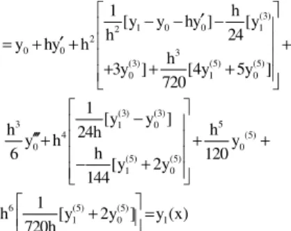
From Eq. 2 it’s easy to verify that: 3

2 4

0 1 0 0 0,2 0 0 0, 4

5

(5) 6

0 0,6

h

S (x ) y hy h a y (x x ) a

6 h

y h a

120

′ ′′′

= + + + + −

+ +

(3)

1 0 0 1

2 2

0 0 3

(3) (5) (5)

0 1 0

(3) (3)

3 1 0 5

4 (5)

0 0

(5) (5)

1 0

6 (5) (5)

1 0 1

1 h

[y y hy ] [y

h 24

y hy h

h

3y ] [4y 5y ] 720

1

[y y ]

h _y _h 24h h _y

h

6 120

[y 2y 144 1

h [y 2y ] y (x)

720h

 

′

− − −

 

′

= + + +

 

+ + +

 

 

 

−

 

′′′+  + +

₋ ₊ 

 

 

 

+ =

 

 

Also it is easy from Eq. 2 and 3 to verify that: Si(xi+1) = yi+1 for i = 0,1,…, n-1:

i

i i,1 2 i 1 i

2 3

(3) (3) (5) (5)

i 1 i i 1 i

( 4) (3) (3) (5) (5)

i 1 i i 1 i

2 2

S (x) a [y y ]

h h

5h h

[y y ] [11y 10y ]

12 360

1 h

S (x) [y y ] [2y y ]

h 6

+

+ +

′′ = − + − +

+ + +

= − + +

and

i

(6) (5) (5) i 1 i

1

S (x) [y y ]

h +

= −

From (5) we have:

(3) (3)

i i 1 i 1

S (x )₊ =y₊ and (5) (5)

i i 1 i 1

S (x )₊ =y₊

From 1 and 2, with using the values of ai,j,

i = 0, 1, …, n-1 and j = 2,4,6 given in the Eq. 9-16, we get:

2

(3) (3) i 1,1 i,1 i 1 i i 1 i

4

(5) (5) i 1 i

2 h

a a [y y ] [y y ]

h 12

h

[y y ]

120

+ + +

+

= − + − + +

− +

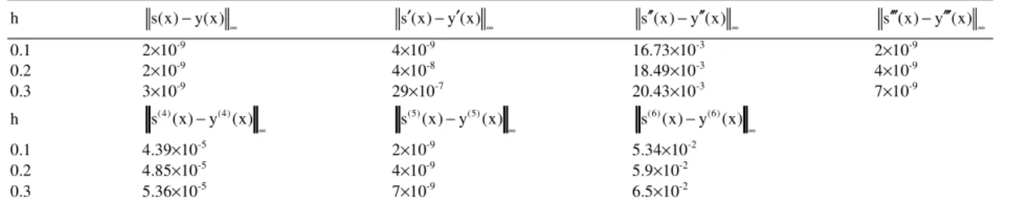
It turns out that the six degree spline which presented in this study, yield approximate solution that is O(h6) as stated in Theorem 2. The results are shown in the Table 1 and 2 for different step sizes h.

Table 1: An absolute maximum error for S(x) and it’s derivative’s for problem 1

h s(x)−y(x)_∞ s (x)′ −y (x)′ _∞ s (x)′′ −y (x)′′ _∞ s (x)′′′ −y (x)′′′ _∞

0.1 1.2×10-10 ₄_×₁₀-9 _1.8_×₁₀-3 ₁_×₁₀-9

0.16 9.6×10-10 4.2×10-8 31.7×10-3 17×10-9

0.2 2×10-9 _1.4_×₁₀-7 _4.19_×₁₀-3 ₆₉_×₁₀-9

h (4) (4)

s (x) y (x)

∞

− (5) (5)

s (x) y (x)

∞

− (6) (6)

s (x) y (x)

∞

−

0.1 4.8×10-5 ₁_×₁₀-9 _5.19_×₁₀-3

0.16 2.18×10-4 ₁₇_×₁₀-9 _13.5_×₁₀-3

(7)

Table 2: An absolute maximum error for S(x) and it’s derivative’s for problem 2

h s(x)−y(x)_∞ s (x)′ −y (x)′ _∞ s (x)′′ −y (x)′′ _∞ s (x)′′′ −y (x)′′′ _∞

0.1 2×10-9 ₄_×₁₀-9 _16.73_×₁₀-3 ₂_×₁₀-9

0.2 2×10-9 ₄_×₁₀-8 _18.49_×₁₀-3 ₄_×₁₀-9

0.3 3×10-9 ₂₉_×₁₀-7 _20.43_×₁₀-3 ₇_×₁₀-9

h (4) (4)

s (x) y (x)

∞

− (5) (5)

s (x) y (x)

∞

− (6) (6)

s (x) y (x)

∞

−

0.1 4.39×10-5 2×10-9 5.34×10-2

0.2 4.85×10-5 ₄_×₁₀-9 _5.9_×₁₀-2

0.3 5.36×10-5 ₇_×₁₀-9 _6.5_×₁₀-2

CONCLUSION

In this study we treat for a first time a lacunary data (0,3,5) by constructing spline function of degree six which interpolates the lacunary data (0,3,5) and the constructed spline function applied to solve the second order initial value problems. Numerical examples, showed that the presented spline function proved their effectiveness in solving the second order initial value problems. Also, we note that, the better error bounds are obtained for a small step size h.

REFERENCES

1. Ahmed, M., M. Eamail, Th. Fawzy and H. Elmoselhi, 1994. Deficient spline function approximation to fourth order differential equations. Applied Math. Modell., 18: 658-664. DOI: 10.1016/0307-904X(94)90390-5

2. Gyovari, J., 1984. Cauchy problem and modified lacunary spline functions. Construct. Theor. Funct., 84: 392-396.

3. Howell, G. and A.K. Varma, 1989. Best error bounds for quartic spline interpolation.

Approximat. Theor., 58: 58-67.

http://portal.acm.org/citation.cfm?id=6941229421 &coll=&dl=ACM

4. Kanth, A.S., V.R. and V. Bhattacharya, 2006. Cubic spline for a class on non-linear singular boundary value problems arising in physiology. Applied Math. Comput., 174: 768-774.

http://cat.inist.fr/?aModele=afficheN&cpsidt= 17570407

5. Khan, A. and T. Aziz, 2003. The numerical solution of third-order boundary value problems using quintic spline. Applied Math. Comput., 137: 253-260.

http://portal.acm.org/citation.cfm?id=640233 .640238

6. Sallam, S. and M.A. Hussien, 1984. Deficient spline function approximation to second-order differential equations. Applied Math. Modell., 6: 408-412.

http://cat.inist.fr/?aModele=afficheN &cpsidt=9163962

7. Saxena, A., 1987. Solution of cauchy's problem by deficient lacunary spline interpolations. Stud. Babes-Bolyai Math., 2: 62-70.

8. Saxena, A. and E. Venturino, 1994. Solving two-point boundary value problems by means of deficient quartic splines. Applied Math. Comput., 66: 25-40.

http://portal.acm.org/citation.cfm?id=202315. 202318

9. Siddiqi, S.S. and G. Akram, 2003. Quintic spline solutions of fourth order boundary value problem,

arXiv. Math. Natl., 1: 1-12.

http://arxiv.org/PS_cache/math/pdf/0306/0306357v 1.pdf

10. Siddiqi, S.S. and G. Akram, 2007. Solutions of tenth-order boundary value problems using eleven degree splines. Applied Math. Comput.,185: 115-127.

http://cat.inist.fr/?aModele=afficheN&cpsidt= 18835411

11. Siddiqi, S.S., G. Akram and S. Nazeem, 2007. Quintic spline solution of linear sixth-order boundary value problems; Applied Math. Comput., 189: 887-892.

http://cat.inist.fr/?aModele=afficheN&cpsidt=187 92784