Electro-osmotic flow of complex fluids in microchannels

(1)

Electro-osmotic flow

of complex fluids in microchannels

by

Samir Hassan Mahmoud Ahmed Sadek

Dissertation submitted to UNIVERSIDADE DO PORTO

For the degree of Doctor of Philosophy in Mechanical Engineering

Supervised by:

Doctor Manuel António Moreira Alves

Professor Fernando Manuel Coutinho Tavares de Pinho

CEFT - Centro de Estudos de Fenómenos de Transporte Departamento de Engenharia Química

Faculdade de Engenharia da Universidade do Porto Portugal

(2)

(3)

(4)

(5)

Abstract

Microfluidic devices are used to manipulate fluids at microscale, with typical dimensions of the order of tens or hundreds of micrometers. Microfluidic flows are usually driven by pressure difference forcing (PDF), electro-osmotic flow (EOF) forcing, with the latter method using electric fields to promote the flow, or a combination of both. Despite the many advantages of EOF, the current knowledge on the use of this technique is still limited especially with complex fluids. The goal of this thesis is to expand both practical and fundamental knowledge on electrically-driven flows, by investigating EOF experimentally and theoretically, using viscoelastic fluids in microscale flow configurations. Newtonian fluids are also used for comparison purposes.

The thesis starts with a review of the concepts of electrokinetic phenomena and their main categories, with emphasis given to EOF. The governing equations that describe EOF for both Newtonian and non-Newtonian fluids, along with the approximation models required to evaluate the distribution of ions within the electric double layer, are also presented. Subsequently, the working principles for each of the EOF operational modes is described, including direct current and alternating current electro-osmotic flow. A detailed review of osmotic flow instabilities is also discussed, with focus given to electro-elastic instabilities which originate from the coupling of electro-elasticity with electro-osmosis.

The first experimental results of this thesis consist of two experimental methods to measure both the electro-osmotic and the electrophoretic mobilities in a straight rectangular microchannel, using micron-sized tracer particles. The first method is based on imposing a pulsed electric field, while the second is based on the use of a sinusoidal electric field. Newtonian fluids are investigated using both methods, whereas for viscoelastic fluids only the pulse method is used. As an extension of that work, a detailed particle-to-particle

(6)

distribution analysis is presented, which investigates the flow behavior of viscoelastic fluids in a straight rectangular microchannel, under the influence of a pulsed electric field.

An analytical solution is presented for oscillatory EOF in a straight microchannel for multi-mode Oldroyd-B fluids. EOF is used to generate small oscillatory deformations, entitled as small amplitude oscillatory shear by electro-osmosis, which can be used as a measuring tool to determine the rheological properties of viscoelastic fluids under shear flow in the linear regime.

The last chapter of results presents an experimental investigation of the conditions that promote the onset of electro-elastic instabilities in straight microchannels incorporating either hyperbolic shaped contractions followed by abrupt expansions, or with symmetrical hyperbolic shaped contractions/expansions. A Newtonian fluid is used as a reference, and the corresponding flows are examined in each of the tested geometrical configurations, whereas viscoelastic fluids are only examined using the former microchannel in both the forward and reverse flow directions.

Keywords: Electro-osmotic mobility, Electrophoretic mobility, Zeta-potential

measurement, Small amplitude oscillatory shear by electro-osmosis (SAOSEO), Electro-elastic instabilities, Newtonian fluids, ViscoElectro-elastic fluids, Particle tracking velocimetry, Flow visualization.

(7)

(8)

(9)

Resumo

Os dispositivos de microfluídica, com dimensões da ordem das dezenas ou centenas de micrómetros, são usados para manipular fluidos à microescala. Os escoamentos à microescala são normalmente promovidos por gradientes de pressão, por electro-osmose usando campos eléctricos, ou por uma combinação de ambos. Apesar das várias vantagens dos escoamentos induzidos por electro-osmose, o actual conhecimento sobre esta técnica ainda é limitado, especialmente usandos fluidos complexos. O objectivo desta tese consiste em expandir o conhecimento prático e fundamental acerca dos escoamentos induzidos electricamente, investigando por via experimental e teórica os escoamentos por electro-osmose usando fluidos viscoelásticos a escoar em microcanais. Fluidos newtonianos são também usados para efectuar comparações.

A dissertação começa com uma revisão dos conceitos associados aos fenómenos electrocinéticos e as suas principais categorias, com ênfase para o escoamento por electro-osmose. As equações governativas que descrevem o escoamento por electro-osmose para fluidos newtonianos e não-newtonianos são também apresentadas, juntamente com os modelos de aproximação necessários para avaliar a distribuição de iões no interior da dupla camada eléctrica. Os princípios de funcionamento para cada um dos modos de operacão do escoamento por electro-osmose são descritos, incluindo escoamento induzido por corrente contínua e escoamento induzido corrente alternada. Uma revisão detalhada das instabilidades em escoamentos por electro-osmose é também apresentada, com particular foco em instabilidades induzidas pela combinação da elasticidade e da electro-osmose.

Os primeiros resultados experimentais apresentados nesta dissertação consistem em dois métodos experimentais usados para medir simultaneamente as mobilidades electro-osmótica e electroforética num canal de secção rectangular, recorrendo a micro-partículas traçadoras. O primeiro método baseia-se na imposição de um campo eléctrico

(10)

pulsado, enquanto o segundo baseia-se no uso de um campo eléctrico sinusoidal. O escoamento de fluidos newtonianos é investigado usando os dois métodos, enquanto para fluidos viscoelásticos apenas se usou o método do campo eléctrico pulsado. Como uma extensão do trabalho anterior, apresenta-se uma análise da distribuição partícula-a-partícula, na qual se investiga o comportamento dos fluidos viscoelásticos num micro-canal rectangular a direito, sob a influência de um campo eléctrico pulsado.

Uma solução analítica é apresentada para escoamento oscilatório induzido por electro-osmose num microcanal de secção rectangular, para fluidos Oldroyd-B multimodo. Um escoamento por electro-osmose é usado para gerar pequenas deformações oscilatórias, denominado por escoamento de corte oscilatório de pequena amplitude por electro-osmose, as quais podem ser usadas para medir as propriedades reológicas de fluidos viscoelásticos em escoamento de corte no regime linear.

O último capítulo de resultados consiste numa investigação experimental das condições que promovem o aparecimento de instabilidades electro-elásticas quer em microcanais a direito, quer em microcanais compostos por uma contracção hiperbólica seguida de uma expansão abrupta, ou com uma contracção hiperbólica seguida de uma expansão também hiperbólica. Um fluido newtoniano foi usado como referência, o qual foi investigado em cada uma das configurações geométricas testadas, enquanto os fluidos viscoelásticos foram apenas usados na primeira configuração, para os dois sentidos de escoamento possíveis.

Palavras-chave: Mobilidade electro-osmótica, Mobilidade electroforética, Medição do

potencial zeta, Escoamento de corte oscilatório de pequena amplitude por electro-osmose, Instabilidades electro-elásticas, Fluidos newtonianos, Fluidos viscoelásticos, Velocimetria por rastreamento de partículas, Visualização do escoamento.

(11)

(12)

(13)

Acknowledgements

I would like to express my special appreciation, gratitude and thanks to the Portuguese Foundation for Science and Technology (FCT) for giving me the opportunity to pursue my PhD degree in the Faculty of Engineering of University of Porto (FEUP), by their financial support through the scholarship SFRH/BD/85971/2012, and to the Transport Phenomena Research Center (CEFT), which made this thesis possible through the facilities and conditions offered to develop my research work.

I would like also to express my sincere gratitude to my advisors, Doctor Manuel Alves and Professor Fernando Pinho, for their continuous guidance and encouragement that helped me in all the moments during my PhD study, and for all the meetings and discussions that helped me to develop my work towards the right direction. Thanks for giving me the opportunity to join your research team (CEFT) which allowed me to grow both as a researcher and as a person. It is my honor to be one of your students. During the time I worked in CEFT, I gained significant amount of valuable knowledge and experience in the fields of microfluidics and complex fluid flows which will help me to progress in my career effectively and productively. I am grateful that I was given such a chance to do cutting edge research in experimental electro-osmotic flow of complex fluids in microchannels. This opportunity will have a great resonance on my academic work in the future.

Thanks also to all my colleagues at CEFT, who helped me to start and become familiar with most of the laboratory equipments, in particular to Patrícia and Francisco (among others), who have been good friends and who always helped me. Thanks for your support, advices and for your friendship.

A special thanks to my family, who is always by my side to motivate me to strive towards my goal with their unconditional support, dedication and encouragement,

(14)

express my gratitude to all of you in a few words. Thanks for all of your patience, sacrifices, and time that you have spent for me. Your prayers for me were what supported me so far. I dedicate this work to my father. I know he would be very proud of me.

I would also like to thank all my closest friends for their friendship and for the good moments that will be saved in my memory from Porto.

At the end, I would like to offer all my best regards and blessings to those who gave me unlimited support during these years to achieve progress towards the completion of this thesis.

(15)

(16)

(17)

Table of Contents

Abstract ... v

Resumo ... ix

Acknowledgements... xiii

Table of Contents ... xvii

List of Figures ... xxiii

List of Tables ... xliii List of Abbreviations ... xlv PART I ... 1

1 INTRODUCTION ... 3

1.1 Research Motivation ... 3

1.2 Objectives ... 4

1.3 Outline of the Thesis ... 5

References ... 6

2 THEORETICAL CONCEPTS ... 9

2.1 Introduction... 9

2.2 Electrokinetic Phenomena ... 10

2.3 Electro-Osmotic Flow (EOF) ... 11

2.3.1 Electrical double layer ... 12

2.3.2 DC electro-osmosis ... 13

2.3.3 AC electro-osmosis ... 21

2.3.4 Advantages of ACEOF ... 25

2.4 Electro-Osmotic Flow Instabilities ... 25

2.4.1 Electrokinetic instabilities ... 26

2.4.2 Electro-elastic instabilities ... 26

(18)

References ... 30

3 LITERATURE REVIEW ON ELECTRO-OSMOTIC FLOW... 37

3.1 Introduction ... 37

3.2 Generalized Newtonian and Viscoelastic Fluid Models ... 37

3.2.1 Inelastic non-Newtonian fluid models ... 37

3.2.2 Viscoelastic fluids ... 39

3.3 Electro-Osmotic Flow of Newtonian Fluids ... 40

3.4 Electro-Osmotic Flow of Generalized Newtonian Fluids ... 41

3.5 Electro-Osmotic Flow of Viscoelastic Fluids ... 45

3.6 Summary ... 48

Reference ... 48

PART II ... 55

4 EXPERIMENTAL TECHNIQUES AND PROCEDURES ... 57

4.2 EOF Experimental Set-up ... 57

4.3 Fabrication of PDMS Microchannels ... 59

4.4 Preparation of Fluids ... 61

4.4.1 Newtonian fluid ... 62

4.4.2 Viscoelastic fluids ... 62

4.5 Physical Characterization of the Solutions ... 63

4.5.1 Electric properties ... 63

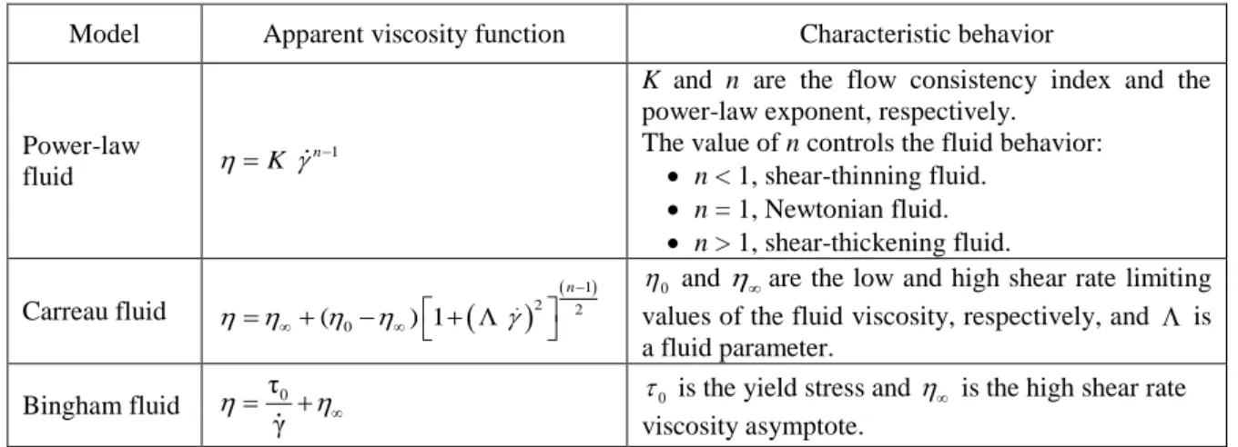
4.5.2 Rheological properties ... 65

4.6 Flow Characterization ... 68

4.6.1 Flow visualization ... 69

4.6.2 Particle tracking velocimetry ... 69

4.7 Electrokinetics: Electrical Equipment ... 70

4.8 Outline of the Experimental and Theoretical Work ... 72

References ... 73

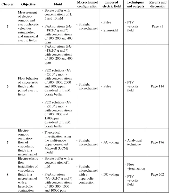
5 MEASUREMENT OF ELECTRO-OSMOTIC AND ELECTROPHORETIC VELOCITIES USING PULSED AND SINUSOIDAL ELECTRIC FIELDS(1) ... 77

5.2 Materials and Methods ... 82

5.2.1 Theory and governing equations ... 82

5.2.2 Microchannel fabrication ... 87

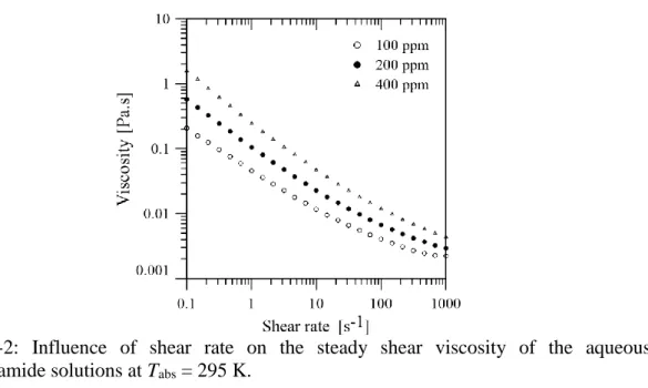
5.2.3 Working fluids ... 88

5.2.4 Experimental set-up and PTV ... 89

(19)

5.3.2 Pulse method evaluation ... 91

5.3.3 Sine-wave method evaluation ... 95

5.3.4 Quantification of the zeta-potential of tracer particles and channel walls... 98

5.3.5 Ionic concentration effect on the zeta-potential ... 100

5.3.6 Advantages and disadvantages of the pulse and sine-wave methods ... 100

5.3.7 Response of viscoelastic fluids to an electric pulse ... 101

5.4 Concluding Remarks ... 105

5.5 Appendix... 105

References ... 107

6 PARTICLE-TO-PARTICLE DISTRIBUTION ANALYSIS OF ELECTROKINETIC FLOWS OF VISCOELASTIC FLUIDS UNDER PULSED ELECTRIC FIELDS ... 111

6.2 Experimental Set-up ... 112

6.2.1 Experimental methods and procedures ... 112

6.2.2 Rheological characterization of the fluids ... 113

6.3 Results and Discussion ... 114

6.3.1 PAA solutions ... 115

6.3.2 PEO solutions with Mw = 5x106 g mol-1 ... 121

6.3.3 PEO solutions with Mw = 8x106 g mol-1 ... 141

6.3.4 Electro-osmotic and electrophoretic mobilities ... 155

References ... 158

7 ELECTRO-OSMOTIC OSCILLATORY FLOW OF VISCOELASTIC FLUIDS IN A MICROCHANNEL ... 161

7.2 Governing Equations and Analytical Solution ... 166

7.2.1 Constitutive equation ... 167

7.2.2 Poisson–Boltzmann equation ... 168

7.2.3 Analytical solution for the multi-mode UCM Model ... 170

7.2.4 Analytical solution for Generic Periodic Forcings ... 175

7.4 On The Use of Electro-Osmosis for SAOS Rheology ... 183

7.5 Conclusions ... 187

7.6 Appendix... 188

References ... 190

8 ELECTRO-ELASTIC FLOW INSTABILITIES OF VISCOELASTIC FLUIDS IN CONTRACTION/EXPANSION MICRO-GEOMETRIES ... 195

(20)

8.2 Experimental Set-up ... 197

8.2.1 Microchannel geometry and fabrication ... 197

8.2.2 Rheological characterization of the fluids ... 199

8.2.3 Experimental methods and procedures ... 201

8.3.1 Relevant dimensionless numbers ... 202

8.3.2 Newtonian fluid ... 203

8.3.3 Non-Newtonian fluids ... 216

References ... 246

PART III ... 251

9 CONCLUSIONS AND FUTURE WORK ... 253

9.1 Conclusions ... 253

(21)

(22)

(23)

List of Figures

Figure 2-1: Illustration of the ions distribution (A) and the potential distribution field of the EDL (B) at the region close to a flat wall surface in contact with a solution containing ions (adapted from [20, 25]). ... 12 Figure 2-2: Schematic diagram of the principle of the DCEOF for a negatively

charged wall (adapted from [30-32]) for a two-dimensional straight microchannel. ... 14 Figure 2-3: Schematic diagram, illustrating (A) the boundary conditions for a

two-dimensional straight microchannel, (B) the flow direction and DCEOF principle of operation (adapted from [33]), and (C) the boundary conditions at the EDL. ... 15 Figure 2-4: Schematic diagram of the principle of ACEOF for an asymmetrical pair

of co-planar electrodes separated by a narrow gap during one full cycle, divided into two equal intervals of times. (A) first intervals of time when the left electrode has a positive polarity: (A-i) electric field on top of a polarized asymmetric electrode; (A-ii) ACEOF net bulk flow field (red dashed line) accompanied by the formation of eddies (blue solid line) above the electrodes surface due to the induced electric field force components. (B) second intervals of time when the electrode polarity is inverted due to the periodic nature of the imposed potential, which creates instabilities responsible for the appearance of eddies such as those shown in Fig. 2-4-(B-ii) (adapted from [30, 42]). ... 23 Figure 2-5: Schematic diagram of the principle of ACEOF. Symmetrical pair of

co-planar electrodes, separated by a narrow gap, during one half-period when the left electrode has a positive polarity. Red dashed line shows the flow streamlines (adapted from [44, 46]). ... 24 Figure 2-6: Schematic diagram for an experimental ACEOF set-up. The electrode

pairs are located and arranged (A) only along the lower wall (reproduced with permission from [41]), (B) along the lower and upper wall (reproduced with permission from [43]). ... 24 Figure 2-7: Illustration of electrophoretic transport phenomenon (adapted from [20,

(24)

Figure 3-1: Shear stress τxy as a function of the shear-rate γ for various purely

viscous fluids and materials in steady Couette flow. ... 38 Figure 3-2: Schematic diagram of a microchannel wall with a depletion layer and

EDL of thicknesses δ and λD, respectively (adapted from [32])... 43

Figure 4-1: The EOF setup used in the experiments. ... 58 Figure 4-2: Schematic diagram of the EOF experimental setup. ... 59 Figure 4-3: PDMS microchannel fabrication procedure: SU-8 mold fabricated using

a chromium mask (A); the SU-8 mold has the inverse structure of the designed microchannels (B), treated by silanizing agent; a PDMS solution with 5:1 ratio of PDMS:curing agent is poured over the SU-8 mold to cure at 80 ºC for 20 minutes (C); the cured PDMS substrate is cut and peeled off from the mold, then punched to create the microchannel inlet/outlet ports (D); a thin layer of PDMS 5:1 solution is poured over a glass substrate and cured at 80 ºC for 2 minutes (E); to obtain the final microchannel, the PDMS substrate is sealed to the glass side which has a thin layer of PDMS (F); finally, the microchannel is kept in the oven at 80ºC for at least 12 hours. ... 61 Figure 4-4: Schematic diagram of the conductivity meter. ... 64 Figure 4-5: Illustration of a rotational rheometer with a cone-plate system. ... 66 Figure 4-6: Illustration of a viscoelastic sample undergoing extensional flow: (A) the

sample at the initial state (t=0, L=L0); (B) the sample after elongation (Δt

= t – t0) has a stretched uniaxial cylindrical filament. ... 67

Figure 4-7: Picture of (A) the function generator (AFG3000 Series, Tektronix) and (B) the high-voltage power amplifier with voltage gain of 200 V/V (Trek, Model 2220) used to generated pulsed and sinusoidal electric fields. ... 71 Figure 4-8: Image of the DC Power Supply (EA-PS 5200-02 A,

EA-Elektro-Automatik-GmbH) used to generated DC electric fields. ... 71 Figure 4-9: Picture of (A) the cables and (B) the wire used to connect the platinum

electrode with the electrical equipment shown in Figs. 4-7 and 4-8. ... 72 Figure 4-10: Calibration curves for an electric field generated using: (A) a function

generator (AFG3000 Series, Tektronix) connected to a high-voltage power amplifier (Trek, Model 2220); (B) a DC Power Supply (EA-PS 5200-02 A, EA-Elektro-Automatik-GmbH). ... 72 Figure 5-1: Schematic representation of the rectangular microchannel, its orientation

relative to the imposed electric field and coordinate system. ... 87 Figure 5-2: Influence of shear rate on the steady shear viscosity of the aqueous

(25)

Figure 5-4: Tracer particle displacement s (a) and velocity u (b) at the centerline of channel A (h = 174 μm), for three applied electric pulse durations (2, 8 and 40 ms) with an amplitude of 440 V/cm. Plots (c) and (d) are a zoomed view of (a) and (b), respectively, at short times. The points represent average experimental values, while the lines are only a guide to the eye. ... 93 Figure 5-5: Regimes in the TP velocity u and displacement s profiles, at the channel

centerline, for an electric pulse with a duration significantly higher than τeo for channel/TP walls with equal polarity zeta-potential ( |ζeo| > |ζep|).

In regime R1, EP is fully-developed, while the EO boundary layer still has

not reached the channel centerline. This is followed by regime R2, where

the EO component is developing and the overall velocity is consequently increasing with time. After the EO velocity component becomes fully-developed, regime R3 starts, which is characterized by a constant velocity.

The last regime (R4) starts after the pulse ends and it is characterized by

the EO velocity decay, since it is assumed that the EP component vanishes very quickly. It is also for this reason that an abrupt increase in the TP velocity is observed at the beginning of R4 – the peak velocity

increase corresponds to the EO velocity component. Adding the velocity in regime R1 (uep) to the peak velocity of R4 (ueo) provides the combined

velocity in regime R3 (ueo + uep). The pulse electric field is active in the

period 0 < t < t3 and t2 ≈ τeo. ... 94

Figure 5-6: Tracer particle displacement s (a) and velocity u (b) at the centerline of channel B (h = 108 μm), for three applied pulse durations (2, 8 and 40 ms) with an amplitude of 440 V/cm. Plots (c) and (d) are a zoomed view of (a) and (b), respectively, at short times. The points represent average experimental values, while the lines are only a guide to the eye. ... 95 Figure 5-7: Tracer particle velocity u at the centerline of (a) channel A (h = 174 μm)

and (b) channel B (h = 108 μm) under a sinusoidal electric field with a peak amplitude of 440 V/cm, for three different frequencies: f = 20, 40 and 80 Hz. The dashed line represents the dimensionless imposed electric signal, while the full lines represent the fitting of Eq. (5.7). The symbols are the average (over cycles and over particles) of experimental data. The best fit found by the algorithm for those conditions gives ueo = 4.3 mm/s

and uep = –3.5 mm/s for channel A and ueo = 4.1 mm/s and uep = –3.2

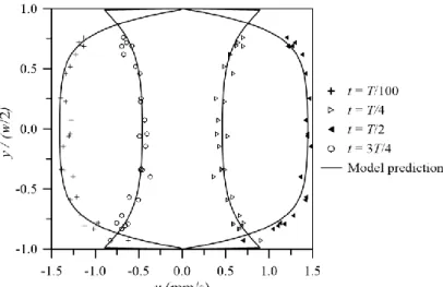
mm/s for channel B. ... 97 Figure 5-8: Spanwise profiles of TP velocity at four different instants of time within

a cycle of period T for channel B (h = 108 μm) under forcing by a sinusoidal electric field with a peak amplitude of 440 V/cm, at f = 40 Hz. The points represent experimental averaged values over several cycles, while the lines represent the analytical prediction of Eq. (5.9) using the best-fit parameters. The channel walls are located at y/(w/2) = ± 1. ... 97 Figure 5-9: Tracer particle velocity components (EO, EP and OBS=EO+EP) as a

function of the applied electric field magnitude, in (a) channel A (h = 174 μm) and (b) channel B (h = 108 μm). The EP/EO mobility is estimated from the slope of the linear fit to the corresponding points (dashed and

(26)

pulse method (at least 20 particles were considered in each experiment). uobs,pulse is the combined (EO +EP) velocity in R3 of Fig. 5-5, whereas

uobs,sine represents the sum of the best-fit parameters (ueo + uep)... 98

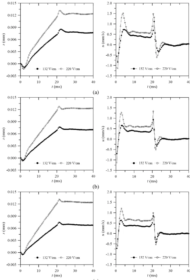
Figure 5-10: wall zeta-potential dependence on the ionic concentration (pC) measured in channel A (h = 174 μm). The points represent experimental data, while the lines are linear fits. ... 100 Figure 5-11: Tracer particle displacement (left side), and velocity u (right

hand-side) at the centerline of channel C (h = 178 μm), for an applied pulse duration of 20 ms with amplitudes of 132 V/cm and 220 V/cm, for polyacrylamide aqueous solutions at the following concentrations: (a) 100 ppm; (b) 200 ppm; (c) 400 ppm. The points represent average experimental values, while the lines are only a guide to the eye. ... 103 Figure 5-12: Regimes in the TP velocity u and displacement s profiles, at the channel

centerline, for a viscoelastic fluid, due to an applied electric pulse. In regime R1, EP dominates. This is followed by regime R2, where the EO

component is still developing to become fully-developed, but before achieving fully-developed flow condition, an overshoot (𝑅2´) occurs and decays. Afterwards regime R3 starts, which is characterized by a constant

velocity. Regime R4 starts after the pulse ends and is characterized by a

zero EP component and before it decays completely, there is a velocity undershoot (𝑅4´) followed by a decay to zero velocity. ... 104 Figure 5-13: Tracer particle velocity components (EO, EP and OBS=EO+EP) as a

function of the applied electric field magnitude, in channel C (h = 178 μm) for PAA solutions with concentrations of 100, 200 and 400 ppm. The dashed lines are a guide to the eye. Error bars represent the standard deviation for the pulse method (at least 20 particles were considered in each experiment). ... 104 Figure 6-1: Schematic diagram illustrating the experimental set-up and the pulse

method. ... 113 Figure 6-2: Influence of shear rate on the steady shear viscosity for aqueous solutions

of PEO of a molecular weight of 5x106_{g mol}-1_{(A) and 8x10}6_{g mol}-1_(B),

both dissolved in a 1 mM borate buffer at Tabs = 295 K. ... 114

Figure 6-3: Tracer particle displacement s for nine different particles (A) – (I) in a solution of PAA (Mw=18x106 g mol-1) at a concentration of 200 ppm,

under a pulsed electric field. The imposed pulse included 8 consecutive cycles (only the last 7 cycles are shown) with 20 ms pulse duration and an amplitude of 88 V/cm. The particles were tracked within 50% of the channel width around the centerline of channel C (h = 178 μm). For reasons of space only 9 particles out of 25 particles are shown (the remaining particles show a similar behavior). The points represent experimental values, while the lines are only a guide to the eye (only one fifth of the points over time are shown). ... 117

(27)

Figure 6-4: Tracer particle displacement s averaged over all cycles, for 25, 13 and 7 particles in a solution of PAA (Mw = 18x106 g mol-1) at a concentration

of 200 ppm, tracked respectively within 50% (A), 30% (B) and 15% (C) of the channel width around the centerline of channel C (h = 178 μm). The analysis was done over 7 consecutive cycles, with 20 ms pulse duration and an amplitude of 88 V/cm. The points represent average experimental values over all cycles, while the lines are only a guide to the eye (only one fourth of the points over time are shown). ... 118 Figure 6-5: Tracer particle displacement s (A) and corresponding

mean-velocity u (B) for TP in a solution of PAA (Mw = 18x106 g mol-1) at a

concentration of 200 ppm, tracked within 50%, 30% and 15% of the channel width around the centerline of channel C (h = 178 μm). The imposed pulse was analyzed over 7 consecutive cycles, with 20 ms pulse duration and an amplitude of 88 V/cm. The points represent average experimental values over the 7 cycles and all particles tracked (global average values), while the lines are only a guide to the eye (only one third of the points over time are shown)... 118 Figure 6-6: Individual tracer particle displacement s averaged over all cycles for

particles in a solution of PAA (Mw = 18x106 g mol-1) at a concentration

of 200 ppm, under a pulsed electric field with amplitudes of 88 V/cm (A), 132 V/cm (B), 176 V/cm (C), and 220 V/cm (D), respectively. The analysis was done for 7 consecutive cycles with 20 ms pulse duration. Particles were tracked within 30% of the channel width around the centerline of channel C (h = 178 μm). The points represent average experimental values, while the lines are only a guide to the eye (only one fourth of the points over time are shown). The number of particles tracked was 13, 15, 12 and 7, respectively for cases from A to D. ... 119 Figure 6-7: Tracer particle displacement s (A) and corresponding

mean-velocity u (B) for an applied pulse duration of 20 ms and amplitudes of 88, 132, 176 and 220 V/cm, for TP in a solution of PAA (Mw=18x106 g

mol-1) at a concentration of 200 ppm. Particles were tracked within 30% of the channel width around the centerline of channel C (h = 178 μm). The points represent average experimental values, while the lines are only a guide to the eye (only half of the points over time are shown). ... 120 Figure 6-8: Tracer particle velocity components (EO, EP and OBS=EO+EP) as a

function of the applied electric field magnitude for a pulse duration of 20 ms, in channel C (h = 178 μm), using a solution of PAA (Mw = 18x106 g

mol-1) at a concentration of 200 ppm. The dashed lines are a guide to the eye. ... 120 Figure 6-9: Tracer particle displacement s for nine different particles (A) – (I) in a

solution of PEO (Mw = 5x106 g mol-1) dissolved in 1 mM borate buffer at

a concentration of 500 ppm, under a pulsed electric field. The imposed pulse included 6 consecutive cycles, with 150 ms pulse duration and an amplitude of 88 V/cm. The particles were tracked within 50% of the channel width around the centerline of channel C (h = 178 μm). For

(28)

remaining particles show a similar behavior). The points represent experimental values, while the lines are only a guide to the eye (only one twentieth of the points over time are shown). ... 124 Figure 6-10: Tracer particle displacement s for different particles (A) – (I) in a

a concentration of 1000 ppm, under a pulsed electric field. The imposed pulse included 6 consecutive cycles, with 150 ms pulse duration and an amplitude of 88 V/cm. The particles were tracked within 50% of the channel width around the centerline of channel C (h = 178 μm). For reasons of space only 9 particles out of 44 particles are shown (the remaining particles show a similar behavior). The points represent experimental values, while the lines are only a guide to the eye (only one twentieth of the points over time are shown). ... 125 Figure 6-11: Tracer particle displacement s for different particles (A) – (I) in a

a concentration of 2000 ppm, under a pulsed electric field. The imposed pulse included 6 consecutive cycles, with 150 ms pulse duration and an amplitude of 88 V/cm. The particles were tracked within 50% of the channel width around the centerline of channel C (h = 178 μm). For reasons of space only 9 particles out of 60 particles are shown (the remaining particles show a similar behavior). The points represent experimental values, while the lines are only a guide to the eye (only one twentieth of the points over time are shown). ... 126 Figure 6-12: Tracer particle displacement s for different particles (A) – (I) in a

a concentration of 3000 ppm, under a pulsed electric field. The imposed pulse included 6 consecutive cycles, with 150 ms pulse duration and an amplitude of 88 V/cm. The particles were tracked within 50% of the channel width around the centerline of channel C (h = 178 μm). For reasons of space only 9 particles out of 60 particles are shown (the remaining particles show a similar behavior). The points represent experimental values, while the lines are only a guide to the eye (only one twentieth of the points over time are shown). ... 127 Figure 6-13: Tracer particle displacement s averaged over all cycles, for 41, 23 and 9

particles in a solution of PEO (Mw = 5x106 g mol-1) dissolved in 1 mM

borate buffer at a concentration of 500 ppm, tracked respectively within 50% (A), 30% (B) and 15% (C) of the channel width around the centerline of channel C (h = 178 μm). The analysis was done over 6 consecutive cycles, with 150 ms pulse duration and an amplitude of 88 V/cm. The points represent average experimental values over all cycles, while the lines are only a guide to the eye (only one twenty-fifth of the points over time are shown). ... 128 Figure 6-14: Tracer particle displacement s (A) and corresponding

mean-velocity u (B) for TP in a solution of PEO (Mw = 5x106 g mol-1) dissolved

(29)

= 178 μm). The imposed pulse was analyzed over 6 consecutive cycles, with 150 ms pulse duration and an amplitude of 88 V/cm. The points represent average experimental values over the 6 cycles and all particles tracked (global average values), while the lines are only a guide to the eye (only one twenty- fifth of the points over time are shown). ... 128 Figure 6-15: Tracer particle displacement s averaged over all cycles, for 44, 29 and

15 particles in a solution of PEO (Mw = 5x106 g mol-1) dissolved in 1 mM

borate buffer at a concentration of 1000 ppm, tracked respectively within 50% (A), 30% (B) and 15% (C) of the channel width around the centerline of channel C (h = 178 μm). The analysis was done over 6 consecutive cycles, with 150 ms pulse duration and an amplitude of 88 V/cm. The points represent average experimental values over all cycles, while the lines are only a guide to the eye (only one twenty- fifth of the points over time are shown). ... 129 Figure 6-16: Tracer particle displacement s (A) and corresponding

in 1 mM borate buffer at a concentration of 1000 ppm, tracked within 50%, 30% and 15% of the channel width around the centerline of channel C (h = 178 μm). The imposed pulse was analyzed over 6 consecutive cycles, with 150 ms pulse duration and an amplitude of 88 V/cm. The points represent average experimental values over the 6 cycles and all particles tracked (global average values), while the lines are only a guide to the eye (only one twenty- fifth of the points over time are shown). ... 129 Figure 6-17: Tracer particle displacement s averaged over all cycles, for 60, 35 and

borate buffer at a concentration of 2000 ppm, tracked respectively within 50% (A), 30% (B) and 15% (C) of the channel width around the centerline of channel C (h = 178 μm). The analysis was done over 6 consecutive cycles, with 150 ms pulse duration and an amplitude of 88 V/cm. The points represent average experimental values over all cycles, while the lines are only a guide to the eye (only one twenty- fifth of the points over time are shown). ... 130 Figure 6-18: Tracer particle displacement s (A) and corresponding

in 1 mM borate buffer at a concentration of of 2000 ppm, tracked within 50%, 30% and 15% of the channel width around the centerline of channel C (h = 178 μm). The imposed pulse was analyzed over 6 consecutive cycles, with 150 ms pulse duration and an amplitude of 88 V/cm. The points represent average experimental values over the 6 cycles and all particles tracked (global average values), while the lines are only a guide to the eye (only one twenty- fifth of the points over time are shown). ... 130 Figure 6-19: Tracer particle displacement s averaged over all cycles, for 60, 59 and

borate buffer at a concentration of 3000 ppm, tracked respectively within 50% (A), 30% (B) and 15% (C) of the channel width around the

(30)

consecutive cycles, with 150 ms pulse duration and an amplitude of 88 V/cm. The points represent average experimental values over all cycles, while the lines are only a guide to the eye (only one twenty- fifth of the points over time are shown). ... 131 Figure 6-20: Tracer particle displacement s (A) and corresponding

in 1 mM borate buffer at a concentration of of 3000 ppm, tracked within 50%, 30% and 15% of the channel width around the centerline of channel C (h = 178 μm). The imposed pulse was analyzed over 6 consecutive cycles, with 150 ms pulse duration and an amplitude of 88 V/cm. The points represent average experimental values over the 6 cycles and all particles tracked (global average values), while the lines are only a guide to the eye (only one twenty- fifth of the points over time are shown). ... 131 Figure 6-21: Individual tracer particle displacement s averaged over all cycles for

borate buffer at a concentration of 500 ppm, under a pulsed electric field with amplitudes of 88 V/cm (A), 132 V/cm (B), 176 V/cm (C), and 220 V/cm (D), respectively. The analysis was done for 6 consecutive cycles with 150 ms pulse duration. Particles were tracked within 30% of the channel width around the centerline of channel C (h = 178 μm). The points represent average experimental values, while the lines are only a guide to the eye (only one twenty-five of the points over time are shown). The number of particles tracked was 23, 17, 20 and 13, respectively for cases from A to D. ... 132 Figure 6-22: Individual tracer particle displacement s averaged over all cycles for

borate buffer at a concentration of 2000 ppm, under a pulsed electric field with amplitudes of 88 V/cm (A), 132 V/cm (B), 176 V/cm (C), and 220 V/cm (D), respectively. The analysis was done for 6 consecutive cycles with 150 ms pulse duration. Particles were tracked within 30% of the channel width around the centerline of channel C (h = 178 μm). The points represent average experimental values, while the lines are only a guide to the eye (only one twenty-five of the points over time are shown). The number of particles tracked was 35, 50, 36 and 34, respectively for cases from A to D. ... 134

(31)

Figure 6-24: Individual tracer particle displacement s averaged over all cycles for particles in a solution of PEO (Mw = 5x106 g mol-1) dissolved in 1 mM

borate buffer at a concentration of 3000 ppm, under a pulsed electric field with amplitudes of 88 V/cm (A), 132 V/cm (B), 176 V/cm (C), and 220 V/cm (D), respectively. The analysis was done for 6 consecutive cycles with 150 ms pulse duration. Particles were tracked within 30% of the channel width around the centerline of channel C (h = 178 μm). The points represent average experimental values, while the lines are only a guide to the eye (only one twenty-five of the points over time are shown). The number of particles tracked was 59, 34, 22 and 20, respectively for cases from A to D. ... 135 Figure 6-25: Tracer particle displacement s (A) and corresponding

mean-velocity u (B) for an applied pulse duration of 150 ms and amplitudes of 88, 132, 176 and 220 V/cm, for TP in a solution of PEO (Mw = 5x106 g

mol-1_{) dissolved in 1 mM borate buffer at a concentration of 500 ppm.}

Plots (C) and (D) are a zoomed view of (A) and (B), respectively, at short times. Particles were tracked within 30% of the channel width around the centerline of channel C (h = 178 μm). The points represent average experimental values, while the lines are only a guide to the eye (only a fraction of the points over time are shown). ... 136 Figure 6-26: Tracer particle displacement s (A) and corresponding

mol-1) dissolved in 1 mM borate buffer at a concentration of 1000 ppm. Plots (C) and (D) are a zoomed view of (A) and (B), respectively, at short times. Particles were tracked within 30% of the channel width around the centerline of channel C (h = 178 μm). The points represent average experimental values, while the lines are only a guide to the eye (only a fraction of the points over time are shown). ... 137 Figure 6-27: Tracer particle displacement s (A) and corresponding

mol-1) dissolved in 1 mM borate buffer at a concentration of 2000 ppm. Plots (C) and (D) are a zoomed view of (A) and (B), respectively, at short times. Particles were tracked within 30% of the channel width around the centerline of channel C (h = 178 μm). The points represent average experimental values, while the lines are only a guide to the eye (only a fraction of the points over time are shown). ... 138 Figure 6-28: Tracer particle displacement s (A) and corresponding

Plots (C) and (D) are a zoomed view of (A) and (B), respectively, at short times. Particles were tracked within 30% of the channel width around the centerline of channel C (h = 178 μm). The points represent average experimental values, while the lines are only a guide to the eye (only a

(32)

Figure 6-29: Flow regimes in the TP velocity u and displacement s profiles at the channel centerline for a viscoelastic fluid (3000 ppm PEO in 1 mM borate buffer) due to an applied electric pulse. In regime R1, EP becomes

fully-developed. This is followed by regime R2, where the EO component is

still developing to become fully-developed in regime R3, which is

characterized by a constant velocity. Regime R4 starts after the pulse ends

and is characterized by a zero EP component and EO decaying to zero over time. ... 140 Figure 6-30: Tracer particle velocity components (EO, EP and OBS=EO+EP) as a

function of the applied electric field magnitude for a pulse duration of 150 ms, in channel C (h = 178 μm), using a solution of PEO (Mw = 5x106

g mol-1) dissolved in 1 mM borate buffer at concentrations of 500, 1000, 2000 and 3000 ppm. The dashed lines are a guide to the eye. ... 140 Figure 6-31: Tracer particle displacement s for different particles (A) – (I) in a

a concentration of 500 ppm, under a pulsed electric field. The imposed pulse included 6 consecutive cycles, with 150 ms pulse duration and an amplitude of 88 V/cm. The particles were tracked within 50% of the channel width around the centerline of channel C (h = 178 μm). For reasons of space only 9 particles out of 52 particles are shown (the remaining particles show a similar behavior). The points represent experimental values, while the lines are only a guide to the eye (only one twenty of the points over time are shown). ... 143 Figure 6-32: Tracer particle displacement s for different particles (A) – (I) in a

a concentration of 1000 ppm, under a pulsed electric field. The imposed pulse included 6 consecutive cycles, with 150 ms pulse duration and an amplitude of 88 V/cm. The particles were tracked within 50% of the channel width around the centerline of channel C (h = 178 μm). For reasons of space only 9 particles out of 60 particles are shown (the remaining particles show a similar behavior). The points represent experimental values, while the lines are only a guide to the eye (only one twenty of the points over time are shown). ... 144 Figure 6-33: Tracer particle displacement s for different particles (A) – (I) in a

a concentration of 1500 ppm, under a pulsed electric field. The imposed pulse included 6 consecutive cycles, with 150 ms pulse duration and an amplitude of 88 V/cm. The particles were tracked within 50% of the channel width around the centerline of channel C (h = 178 μm). For reasons of space only 9 particles out of 60 particles are shown (the remaining particles show a similar behavior). The points represent experimental values, while the lines are only a guide to the eye (only one twenty of the points over time are shown). ... 145 Figure 6-34: Tracer particle displacement s averaged over all cycles, for 52, 33 and

(33)

50% (A), 30% (B) and 15% (C) of the channel width around the centerline of channel C (h = 178 μm). The analysis was done over 6 consecutive cycles, with 150 ms pulse duration and an amplitude of 88 V/cm. The points represent average experimental values over all cycles, while the lines are only a guide to the eye (only one twenty-five of the points over time are shown). ... 146 Figure 6-35: Tracer particle displacement s (A) and corresponding

in 1 mM borate buffer at a concentration of 500 ppm, tracked within 50%, 30% and 15% of the channel width around the centerline of channel C (h = 178 μm). The imposed pulse was analyzed over 6 consecutive cycles, with 150 ms pulse duration and an amplitude of 88 V/cm. The points represent average experimental values over the 6 cycles and all particles tracked (global average values), while the lines are only a guide to the eye (only one twenty-two of the points over time are shown)... 146 Figure 6-36: Tracer particle displacement s averaged over all cycles, for 60, 38 and

borate buffer at a concentration of 1000 ppm, tracked respectively within 50% (A), 30% (B) and 15% (C) of the channel width around the centerline of channel C (h = 178 μm). The analysis was done over 6 consecutive cycles, with 150 ms pulse duration and an amplitude of 88 V/cm. The points represent average experimental values over all cycles, while the lines are only a guide to the eye (only one twenty-five of the points over time are shown). ... 147 Figure 6-37: Tracer particle displacement s (A) and corresponding

in 1 mM borate buffer at a concentration of 1000 ppm, tracked within 50%, 30% and 15% of the channel width around the centerline of channel C (h = 178 μm). The imposed pulse was analyzed over 6 consecutive cycles, with 150 ms pulse duration and an amplitude of 88 V/cm. The points represent average experimental values over the 6 cycles and all particles tracked (global average values), while the lines are only a guide to the eye (only one twenty-two of the points over time are shown)... 147 Figure 6-38: Tracer particle displacement s averaged over all cycles, for 60, 42 and

borate buffer at a concentration of 1500 ppm, tracked respectively within 50% (A), 30% (B) and 15% (C) of the channel width around the centerline of channel C (h = 178 μm). The analysis was done over 6 consecutive cycles, with 150 ms pulse duration and an amplitude of 88 V/cm. The points represent average experimental values over all cycles, while the lines are only a guide to the eye (only one twenty-five of the points over time are shown). ... 148 Figure 6-39: Tracer particle displacement s (A) and corresponding

(34)

C (h = 178 μm). The imposed pulse was analyzed over 6 consecutive cycles, with 150 ms pulse duration and an amplitude of 88 V/cm. The points represent average experimental values over the 6 cycles and all particles tracked (global average values), while the lines are only a guide to the eye (only one twenty-two of the points over time are shown). ... 148 Figure 6-40: Individual tracer particle displacement s averaged over all cycles for

borate buffer at a concentration of 1500 ppm, under a pulsed electric field with amplitudes of 88 V/cm (A), 132 V/cm (B), 176 V/cm (C), and 220 V/cm (D), respectively. The analysis was done for 6 consecutive cycles with 150 ms pulse duration. Particles were tracked within 30% of the channel width around the centerline of channel C (h = 178 μm). The points represent average experimental values, while the lines are only a guide to the eye (only one twenty-five of the points over time are shown). The number of particles tracked was 42, 46, 50 and 44, respectively for cases from A to D. ... 151 Figure 6-43: Tracer particle displacement s (A) and corresponding

Plots (C) and (D) are a zoomed view of (A) and (B), respectively, at short times. Particles were tracked within 30% of the channel width around the centerline of channel C (h = 178 μm). The points represent average experimental values, while the lines are only a guide to the eye (only a

(35)

Figure 6-44: Tracer particle displacement s (A) and corresponding mean-velocity u (B) for an applied pulse duration of 150 ms and amplitudes of 88, 132, 176 and 220 V/cm, for TP in a solution of PEO (Mw = 8x106 g

Plots (C) and (D) are a zoomed view of (A) and (B), respectively, at short times. Particles were tracked within 30% of the channel width around the centerline of channel C (h = 178 μm). The points represent average experimental values, while the lines are only a guide to the eye (only a fraction of the points over time are shown). ... 153 Figure 6-45: Tracer particle displacement s (A) and corresponding

mol-1) dissolved in 1 mM borate buffer at a concentration of 1500 ppm. Plots (C) and (D) are a zoomed view of (A) and (B), respectively, at short times. Particles were tracked within 30% of the channel width around the centerline of channel C (h = 178 μm). The points represent average experimental values, while the lines are only a guide to the eye (only a fraction of the points over time are shown). ... 154 Figure 6-46: Tracer particle velocity components (EO, EP and OBS=EO+EP) as a

function of the applied electric field magnitude for a pulse duration of 150 ms, in channel C (h = 178 μm), using a solution of PEO (Mw = 8x106

g mol-1) dissolved in 1 mM borate buffer at concentrations of 500, 1000 and 1500 ppm. The dashed lines are a guide to the eye... 155 Figure 7-1: Schematic diagram, illustrating the microchannel dimensions, coordinate

system, and the induced potential boundary conditions. ... 167 Figure 7-2: Profiles of the normalized velocities components for several

1 2

Π /  1, 0, 1 for a Newtonian fluid at Re = 0.01,  =100, ω t=

0 and m = 1. ... 177 Figure 7-3: Profiles of the normalized velocity for a Newtonian fluid (left-hand side)

and viscoelastic fluid, λ ω = 5 (right-hand side) for ω t= 0, Π = 0 and m = 1, as a function of ,Reynolds and Mach numbers: (A-i) Re = 0.01, M = 0 (B-i) Re = 1, M = 0 (C-i) Re = 10, M = 0 (D-i) Re = 100, M = 0 and (A-ii) Re = 0.01, M = 0.22 (B-ii) Re = 1, M = 2.2 (C-ii) Re = 10, M = 7 (D-ii) Re = 100, M = 22. ... 180 Figure 7-4: Profiles of the normalized velocity components for different λ ω, at the

instant of maximum imposed electric potential (ω t = 0), for Re = 0.01, Π = 0, m = 1 and different values of  : (A) λ ω = 0, M = 0 (B) λ ω = 5, M = 0.22 (C) λ ω = 10, M = 0.32 (D) λ ω = 20, M = 0.45 (E) λ ω = 40, M = 0.63 and (F) λ ω = 60, M = 0.77. ... 181 Figure 7-5: Profiles of the normalized velocity components for a Newtonian fluid

(left-hand side) and a viscoelastic fluid, λ ω = 5 (right-hand side) for 

= 100, Π = 0, m = 1, and as a function of ω t and Reynolds number: (A) Re = 0.01, (B) Re = 10. ... 182

(36)

Figure 7-6: Variation of the normalized velocity at y0.95 with ω t / 2π for Re = 0.01,  = 100, Π = 0, m = 1 and as a function of λ ω. ... 182 Figure 7-7: Schematic diagram illustrating small amplitude oscillatory

electro-osmotic shear flow (SAOSEO) under operating conditions of very small Re and large  , leading to a flow with similar characteristics to that of SAOS in rotational shear. ... 183 Figure 8-1: Schematic representation of the four microchannels used: Two

microchannels (H2, and H3) have a hyperbolic contraction followed by an

abrupt expansion, with εH = 2 (A) and εH = 3 (B); two microchannels

(H2Sym and H3Sym) have a hyperbolic contraction followed by an identical

hyperbolic shaped expansion, with εH = 2 (C) and εH = 3 (D). ... 198

Figure 8-2: Schematic representation and relevant dimensions for a microchannel with hyperbolic contraction and expansion. ... 199 Figure 8-3: Shear viscosity curves in steady shear flow for all fluids at Tabs = 295 K... 200

Figure 8-4: Flow visualizations using an aqueous solution of 1 mM borate buffer, seeded with 1.0 µm TP, using microchannel H2 (A, B and C) and H2Sym

(D, E and F), under imposed DC potential differences of 5, 30 and 90 V, at Tabs = 295 K. The red dashed lines represent the numerically predicted

streamlines for a purely electro-osmotic flow of a Newtonian fluid, and the yellow lines are used to highlight the microchannel walls. The yellow arrow indicates the flow direction. The Reynolds number was computed at the throat for microchannels H2 and H2Sym and are Re = 0.13 and 0.11,

respectively, at the higher voltage. ... 204 Figure 8-5: Flow visualizations using an aqueous solution of 1 mM borate buffer,

seeded with 1.0 µm TP, using microchannel H3 (A, B and C) and H3Sym

(D, E and F), under imposed DC potential differences of 5, 20 and 60 V, at Tabs = 295 K. The red dashed lines represent the numerically predicted

streamlines for a purely electro-osmotic flow of a Newtonian fluid, and the yellow lines are used to highlight the microchannel walls. The yellow arrow indicates the flow direction. The Reynolds number was computed at the throat for microchannels H3 and H3Sym and are Re = 0.084 and

0.049, respectively, at the higher voltage. ... 205 Figure 8-6: Flow visualizations using an aqueous solution of 1 mM borate buffer,

seeded with 0.5 µm TP, using microchannel H2 (A, B and C), H2Sym (D,

E and F), H3 (G, H and I) and H3Sym (J, K and L), under imposed DC

potential differences of 30, 60 and 120 V, at Tabs = 295 K. The red dashed

lines represent the numerically predicted streamlines for a purely electro-osmotic flow of a Newtonian fluid, and the yellow lines are used to highlight the microchannel walls. The yellow arrow indicates the flow direction. ... 206 Figure 8-7: Centerline velocity profiles computed numerically for a two-dimensional

and a three-dimensional geometry at several depths; z/H = 0.0, 0.05, 0.2, 0.3, 0.5 , assuming a purely EOF of a Newtonian fluid, with an imposed

(37)

DC voltage of 30 V in microchannels H2 (A) and H2Sym (B), and 20 V in

microchannels H3 (C) and H3Sym (D). The black arrow indicates the flow

direction. ... 208 Figure 8-8: Snapshots at several depths, starting from the lower wall at z/H = 0.0 (A)

up to the upper wall at z/H = 1.0 (O) in microchannel H2, for a no-flow

condition. ... 210 Figure 8-9: Centerline velocity profile measured at several depths (A) z/H = 0.05,

0.15, 0.30, 0.50, 0.70, 0.85, 0.95 , and (B) corresponding normalized velocity profiles for each curve and comparison with the velocity profile computed numerically for 2D flow, in microchannel H2 at an imposed

potential difference of 30 V using the 1 mM borate buffer with dye added. The black arrow to indicates the flow direction. ... 211 Figure 8-10: Centerline velocity profiles measured at z/H = 0.15, in microchannel H2

(R1 and R2, each run was done in a new microchannel) using the 1 mM borate buffer with and without dye, for imposed potential differences of 5, 10, 30 and 60 V (A), and (B) corresponding normalized velocity profiles and comparison with the velocity profile computed numerically for 2D flow. The black arrow indicates the flow direction. ... 212 Figure 8-11: Fully-developed velocity (v1) at the upstream channel (A) and maximum

velocity (v2) at the throat of the contraction (B) for microchannel H2,

using the 1 mM borate buffer with and without dye. ... 212 Figure 8-12: Centerline velocity profiles measured at z/H = 0.15, in microchannel H2

(R1 and R2) using the 1 mM borate buffer, for imposed potential differences of 5, 10, 30, 60 and 90 V (A), and (B) corresponding normalized velocity profiles and comparison with the velocity profile computed numerically for 2D flow. The black arrow indicates the flow direction, and the Reynolds number at the throat is about 0.13 for 90 V. .... 213 Figure 8-13: Centerline velocity profiles measured at z/H = 0.15, in microchannel

H2Sym (R1 and R2) using the 1 mM borate buffer, for imposed potential

differences of 5, 10, 30, 60 and 90 V (A), and (B) corresponding normalized velocity profiles and comparison with the velocity profile computed numerically for 2D flow. The black arrow indicates the flow direction, and the Reynolds number at the throat is about 0.11 for 90 V. .... 214 Figure 8-14: Centerline velocity profiles measured at z/H = 0.15, in microchannel H3

(R1 and R2) using the 1 mM borate buffer, for imposed potential differences of 5, 10, 30, 60 and 90 V (A), and (B) corresponding normalized velocity profiles and comparison with the velocity profile computed numerically for 2D flow. The black arrow indicates the flow direction, and the Reynolds number at the throat is about 0.084 for 60 V. ... 214 Figure 8-15: Centerline velocity profiles measured at z/H = 0.15, in microchannel

H3Sym (R1, R2, R3 and R4) using the 1 mM borate buffer, for imposed

(38)

normalized velocity profiles and comparison with the velocity profile computed numerically for 2D flow. The black arrow indicates the flow direction, and the Reynolds number at the throat is about 0.049 for 60 V. ... 215 Figure 8-16: Variation with imposed potential difference of the fully-developed

velocity (v1) at the upstream channel (A) and maximum velocity (v2) at

the throat of the contraction (B) for microchannels H2, H2Sym, H3, and

H3Sym, using the 1 mM borate buffer with dye. ... 216

Figure 8-17: Flow visualizations using a viscoelastic aqueous solution of PAA (Mw =

5x106 g mol-1) at a concentration of 100 ppm, seeded with 1.0 µm TPs, using microchannel H2. The flow is in the forward direction, from left to

right, at Tabs = 295 K, and under DC potential differences of 5 V (A), 10

V (B), 20 V (C), 30 V (D), 40 V (E), 50 V (F), 60 V (G), and 70 V (H). The yellow arrow indicates the flow direction. ... 217 Figure 8-18: Flow visualizations using a viscoelastic aqueous solution of PAA (Mw =

V (B), 30 V (C), 60 V (D), 80 V (E), 100 V (F), 120 V (G), 140 V (H), 160 V (I), 180 V (J), and 200 V (K). The yellow arrow indicates the flow direction. ... 218 Figure 8-19: Flow visualizations using a viscoelastic aqueous solution of PAA (Mw =

5x106_{g mol}-1_{) at a concentration of 100 ppm, seeded with 1.0 µm TPs,}

using microchannel H2. The flow is in the reverse direction, from left to

5x106 g mol-1) at a concentration of 1000 ppm, seeded with 1.0 µm TPs, using microchannel H2. The flow is in the reverse direction, from left to

V (B), 30 V (C), 40 V (D), 60 V (E), 80 V (F), 100 V (G), 120 V (H), 140 V (I), 160 V (J), and 180 V (K). The yellow arrow indicates the flow direction. ... 221 Figure 8-22: Flow visualizations using a viscoelastic aqueous solution of PAA (Mw =

(39)

V (B), 15 V (C), 20 V (D), 25 V (E), 30 V (F), 35 V (G), and 40 V (H). The yellow arrow indicates the flow direction. ... 222 Figure 8-23: Evolution with time of flow behavior for an imposed DC potential

difference of 25V in microchannel H2, using an aqueous solution of PAA

(Mw = 5x106 g mol-1) at a concentration of 10000 ppm. The flow is in the

reverse direction from left to right, at Tabs = 295 K. The yellow arrow

indicates the flow direction. ... 223 Figure 8-24: Flow visualizations using a viscoelastic aqueous solution of PAA (Mw =

V (B), 20 V (C), 30 V (D), 40 V (E), and 50 V (F). The yellow arrow indicates the flow direction. ... 225 Figure 8-25: Flow visualizations using a viscoelastic aqueous solution of PAA (Mw =

right, at Tabs = 295 K, and under DC potential differences of 2.5 (A), 5

(B), 7.5 (C), 10 (D), 12.5 (E), 15 (F), 20 (G), 40 (H) 60 (I), 80 (G), 100 V (K). The yellow arrow indicates the flow direction. ... 226 Figure 8-26: Flow visualizations using a viscoelastic aqueous solution of PAA (Mw =

right, at Tabs = 295 K, and under DC potential differences of 2.5 (A), 5

(B), 7.5 (C), 10 (D), 12.5 (E), 15 (F), 20 (G), 40 (H) 60 (I), 80 (G), 100 V (K). The yellow arrow indicates the flow direction. ... 227 Figure 8-27: Schematic representation of flow instabilities (in red), showing the flow

direction within the separated flow regions, for microchannel H3 using

PAA (Mw=5x106 g mol-1) at a concentration of 1000 ppm. The flow is in

the forward direction, from left to right, at Tabs = 295 K, under a DC

potential difference of 10 V. ... 228 Figure 8-28: Flow visualizations using a viscoelastic aqueous solution of PAA (Mw =

V (B), 30 V (C), 40 V (D), 60 V (E), 80 V (F), 100 V (G), 120 V (H), 140 V (I), 160 V (J), and 180 V (K). The yellow arrow indicates the flow direction. ... 229 Figure 8-29: Schematic representation of flow instabilities (in red), showing the flow

direction within the separated flow regions, for microchannel H3 using

PAA (Mw=5x106 g mol-1) at a concentration of 100 ppm. The flow is in

the reverse direction, from left to right, at Tabs = 295 K, under a DC