U
NIVERSIDADE DE
L
ISBOA
Faculdade de Ciˆencias
Departamento de Inform´atica
Percussion Graphs : An Automated Approach for
Percussion Composition
Louis Philippe Sim˜oes Castelo Branco Lopes
MESTRADO EM ENGENHARIA INFORM ´
ATICA
Especializac¸˜ao em Interacc¸˜ao e Conhecimento
U
NIVERSIDADE DE
L
ISBOA
Faculdade de Ciˆencias
Departamento de Inform´atica
Percussion Graphs : An Automated Approach for
Percussion Composition
Louis Philippe Sim˜oes Castelo Branco Lopes
DISSERTAC
¸ ˜
AO
Projecto orientado pelo Prof. Doutor Paulo Jorge Vaz Cunha Dias Urbano
MESTRADO EM ENGENHARIA INFORM ´
ATICA
Especializac¸˜ao em Interacc¸˜ao e Conhecimento
Acknowledgments
It has been a long road since I was freshman just entering college for the first time, and learning the proverbial ropes around campus (which I came to know like the back of my hand, after all these years). I know that I would have never accomplished any of this without the help of all my family and friends who molded me into the person I am today and in a way, I write this as a great big thank you for their continued influence on my life.
I would firstly like to thank my family, my mother and my father who have always watched over me and guided me my whole life, and of course my brother and his beautiful wife, who have always been there whenever I needed them.
I would also like to thank all my friends and coworkers here at LabMAg who helped me throughout my college career and thesis. I’d like to particularly thank Andr´e Bas-tos, Jo˜ao Costa, Geraldo Nascimento, Chrisitan Marques, Davide Nunes, Bruno Correia, Marco Lourenc¸o, Gonc¸alo Cruchinho, Henrique Morais, Rui Flores, Jo˜ao Lobo, Frede-rico Miranda, Jo˜ao Lopes, Carlos ´Alvares, Carlos Teixeira, Diogo Serrano, Dinis Premji and Joaquim Tiago Reis.
I’d also like to thank my music teacher Emanuel Sousa who taught me everything I know and love about the guitar, music and musical composition. I’d also like to thank Sara Salazar, Francisco Gonc¸alves, Andr´e Batista and David Oliveira, who have given me some musical sanity along all my years playing the electric guitar.
I also couldn’t forget my friends who have been with me since before I even dreamed of college life and most likely if it weren’t for them I wouldn’t even be here today, par-ticularly Marlene Martins, Fabio Reis and my 10oto 12ograde teacher Paulo Gonc¸alves, who was more than a teacher but a great friend to all of us in our old computer science group.
Finally I would also like to thank my thesis coordinator and professor Paulo Urbano, who gave me the liberty to explore the theme of this work and was not only a great mentor but a great friend.
Resumo
A composic¸˜ao m´usical ´e um processo art´ıstico interessante, que envolve n˜ao s´o cria-tividade mas tamb´em experimentac¸˜ao. Neste trabalho propomos um sistema que integra v´arios conceitos de sistemas de m´usica generativa, com um particular foco na integrac¸˜ao do utilizador.
Ao contr´ario de outros sistemas de m´usica generativa, principalmente os sistemas de m´usica gen´etica, ao qual o ´unico papel que o utilizador tem sobre as m´usicas ´e de avaliador (avaliar a m´usicalidade de cada ritmo gerado), o nosso sistema ir´a permitir ao utilizador fazer parte do processo criativo e criar os seus pr´oprios ritmos, que ser˜ao pre-ponderantes depois no processo generativo musical.
Os principais objectivos deste trabalho foram:
• Sistema em que o utilizador seria mais do que um avaliador ou juiz r´ıtmico e fazer parte do processo criativo m´usical;
• Fornecer ao utilizador m´ultiplas formas de gerar a m´usica;
• A m´usica gerada n˜ao dever´a ser uma cacofonia de sons, mas apresentar alguma es-trutura m´usical.
Introduzimos o conceito de ”Grafos de Percuss˜ao”, que ´e uma sistema de composic¸˜ao h´ıbrido, misturando elementos interactivos (dependem do utilizador) com elementos mais autom´aticos ou generativos. Um grafo percursivo n˜ao ´e mais do que um grafo dirigido ao qual se associam, tanto aos n´os como `as conex˜oes, ritmos percursivos. Cada n´o est´a associado a um ritmo criado por um utilizador, enquanto cada conex˜ao, representa uma sequˆencia de ritmos. A ideia do grafo de percuss˜ao era criar um processo de composic¸˜ao intuitivo no qual o utilizador pudesse criar v´arios ritmos e interlig´a-los. A cada n´o o utilizador ir´a associar um ritmo percursivo, enquanto os ritmos musicais associados ´as conex˜oes ir˜ao ser fruto de um processo generativo.
Os ritmos dos n´os s˜ao criados pelo utilizador atrav´es de uma caixa de ritmos, que consiste numa grelha de 16 linhas por 16 colunas. As linhas representam os v´arios ins-trumentos de percuss˜ao dispon´ıveis enquanto as colunas representam todos os tempos
dispon´ıveis, neste caso um tempo ´e uma semicolcheia. Quando um ritmo ´e criado o utili-zador ter´a que apenas transferir o ritmo para a aplicac¸˜ao ao qual este depois transformar´a num n´o do grafo.
A cada conex˜ao vai corresponder uma sequˆencia de ritmos percursivos que repre-senta a progress˜ao musical entre o ritmo do seu n´o inicial at´e ao ritmo do seu n´o final. Este ritmo progressivo corresponde ao rasto do processo de optimizac¸˜ao, que ´e formado pela sequˆencia de ritmos obtidas em cada iterac¸˜ao do processo de optimizac¸˜ao. Imple-mentamos trˆes t´ecnicas de optimizac¸˜ao para gerar os ritmos das conex˜oes, que foram: Algoritmo Gen´etico, Trepa Colinas e o Trepa Colinas Estoc´astico. Estes foram escolhi-dos pela capacidade de criar diversidade tanto a tamanho e natureza das sequˆencias escolhi-dos ritmos gerados.
Todos os optimizadores utilizaram a mesma func¸˜ao objectivo que ´e uma medida de semelhanc¸a de qualquer ritmo objectivo (ritmo final). Nomeadamente os instrumentos que s˜ao comuns aos dois ritmos, os tempos comuns (o tempo a que uma nota ´e tocada) e notas que s˜ao exactamente iguais tanto em instrumento como tempo. A func¸˜ao ob-jectivo consoante estas caracter´ısticas ir´a dar uma classificac¸˜ao entre 1 a 10, 10 sendo exactamente semelhante com o ritmo final. Logo como ´e de se esperar, os algoritmos generativos tˆem como func¸˜ao progredir os ritmos atrav´es desta avaliac¸˜ao r´ıtmica. No en-tanto, o objectivo n˜ao ´e chegar ao ritmo final o mais eficientemente poss´ıvel, mas de forma a que este seja capaz de criar ritmos interm´edios que subjectivamente s˜ao ”valiosos”para o utilizador.
Pode existir v´arias situac¸˜oes em que uma sequˆencia r´ıtmica poder´a ser demasiado longa ou repetitiva. Para combater esta situac¸˜ao introduzimos o conceito de filtros que permitem ao utilizador editar as v´arias conex˜oes geradas, como por exemplo cortar uma parte r´ıtmica da conex˜ao (O Filtro Corte entre dois Pontos), eliminar todos os ritmos que tˆem um valor de avaliac¸˜ao menor do que X (O Filtro por Classificac¸˜ao), eliminar repetic¸˜oes (O Filtro por Repetic¸˜ao).
O processo de composic¸˜ao musical n˜ao se resume `a gerac¸˜ao do grafo percursivo. O grafo cont´em todos elementos da composic¸˜ao musical, mas a pr´opria musica ser´a o resul-tado de uma travessia do grafo. Conceptualiz´amos dois tipos de travessia, definindo dois n´os como sendo dois extremos de um caminho (inicio e fim) ou ent˜ao fazer uma traves-sia que passa por todos os ritmos uma ´unica vez, problema an´aloga ao celebre caixeiro viajante.
Se o utilizador decidir definir dois extremos de um caminho, um processo que cham´amos de ”Path Finding”, a aplicac¸˜ao retornar´a uma m´usica (lista de ritmos) com todas as co-nex˜oes interm´edias que satisfazem um caminho entre esses dois extremos (caso seja poss´ıvel). O utilizador ter´a `a sua disposic¸˜ao 3 tipos de algoritmos de ”Path Finding”: Procura em Largura (Breath-first Search), Procura em Profundidade (Depth-first Search) e a Procura Aleat´oria (Random Search). Dependendo do grafo estas 3 opc¸˜oes podem
retornar resultados completamente diferentes, o que ajuda sempre na variedade musical. Neste tipo de travessias os n´os podem ser repetidos.
Caso o utilizador escolher a opc¸˜ao do caixeiro viajante, o processo ir´a primeiro de tudo gerar conex˜oes novas para criar um grafo totalmente conexo. Isto ´e necess´ario para que o algoritmo seja poss´ıvel, e para n˜ao obrigar o utilizador a ter que interligar todos os n´os manualmente. Quando o processo de criac¸˜ao do grafo terminar, calculamos um circuito usando um m´etodo de pesquisa local, o 2-Opt, utilizado com grande sucesso no problema cl´assico do caixeiro viajante.
Para que o utilizador seja capaz de utilizar todas estas caracter´ısticas foi necess´ario criar um interface, onde o utilizador pudesse ter f´acil acesso a todas a opc¸˜oes e carac-ter´ısticas do programa. Esta interface permite:
• Criar os n´os, manipul´a-los, interliga-los com conex˜oes;
• Ouvir conex˜oes e n´os;
• Escolher o algoritmo generativo de optimizac¸˜ao para preencher as conex˜oes;
• Gerar a lista de ritmos para as conex˜oes existentes;
• Aplicar filtros nas conex˜oes;
• Escolher o tipo de travessia;
• Definir os extremos para a travessia ponto a ponto e gerar o resultado;
• Obter a lista de ritmos do algoritmo caixeiro viajante e ouvir o resultado;
• Ouvir as Travessias.
Todos estes conceitos ser˜ao explicados e detalhados neste trabalho, incluindo detalhes de implementac¸˜ao, a investigac¸˜ao e experimentac¸˜ao do conceito de grafo de percuss˜ao e um manual de utilizac¸˜ao do sistema. Este trabalho tamb´em inclu´ı uma secc¸˜ao de dis-cuss˜ao e uma apreciac¸˜ao musical dos resultados obtidos, como a musicalidade, tempo de gerac¸˜ao e an´alise dos resultados do path finding. O sistema tamb´em foi testado com um grupo de utilizadores (m´usicos e n˜ao m´usicos) ao qual este trabalho tamb´em descrever´a as experiˆencias dos utilizadores e a sua apreciac¸˜ao musical.
Palavras-chave: M´usica, Percuss˜ao, Grafo, Generativo, Automac¸˜ao
Abstract
Musical composition is an interesting artistic process, which can involve a lot of ex-perimentation with various known musical concepts. In this work we propose a system that tries to integrate various aspects of music generation and automation systems, but with a focus on integrating the user into the music creation process. Unlike systems who cast users into a musical arbiter role, our system generates music in accordance to user created music.
We named this system Percussion Graphs, and consists of a musical graph repre-sentation of user created rhythms and generated rhythms. A graph contains two main components: The Node component (which are User Created Rhythms) and a Connec-tion component (which is a List of Generated Rhythms). The idea is to have users create rhythms, that can then be connected with each other. These connections are the rhythm generation process, and they consist of a slow progressive transformation process of one rhythm into another, in this case two user created rhythms.
A user will be able to control multiple aspects of the percussion graph such as node manipulation and creation, node connection, choosing the rhythm generating methodol-ogy from multiple available methodologies, traveling the percussion graph and hearing the generated solutions. We also implemented editing options, called filters, that will let the user trim and edit connections to his or her liking.
In this work we will explain on how the percussion graph and all of its features were implemented and how they work (internally and usability wise). We also talk about on what led us to follow this specific modus operandi. We also discuss the experiences of several users during their test run with the percussion graph system, and their thoughts on the generated rhythms and the system itself.
Keywords: Music, Percussion, Graph, Generative, Automation
Contents
List of Figures xviii
List of Tables xxi
1 Introduction 1
1.1 Motivation . . . 3
1.2 Objectives . . . 3
1.3 Contributions . . . 4
1.4 Document Structure . . . 4
2 State of the Art 7 2.1 Horowitz’s Genetic Algorithm Rhythms . . . 8
2.2 CONGA . . . 8
2.3 The Evolving Drum Machine . . . 9
2.4 Beatrix - The Amorphous Drum Ensemble . . . 9
2.5 GenJam . . . 10
2.6 Coming Together . . . 10
3 Percussion Graphs 13 3.1 A Percussion Graph . . . 14
3.1.1 The Node . . . 14
3.1.2 The Connection - The Directed Edge . . . 16
3.2 Automated Connection - Generating Rhythms for the Directed Edge . . . 16
3.3 The Objective Function: Measuring the Rhythms Similarity . . . 18
3.3.1 Measuring Rhythm Similarity . . . 18
3.4 Optimization Processes . . . 22
3.4.1 Genetic Evolution Process . . . 22
3.4.2 Hill Climbing Process . . . 27
3.4.3 Stochastic Hill Climbing Process . . . 28
3.4.4 Optimization Filters . . . 29
4 Traveling the Percussion Graph 35
4.1 Path Traveling Algorithms . . . 36
4.1.1 Breadth-first Search . . . 37
4.1.2 Depth-first Search . . . 39
4.1.3 Random Search . . . 41
4.2 Traveling Salesman with 2-Opt . . . 43
4.2.1 Initializing the TSP Algorithm . . . 44
4.2.2 The Nearest Neighbor Algorithm . . . 44
4.2.3 The 2-Opt Optimization . . . 44
5 The Percussion Graph Application 49 5.1 The Drum Machine . . . 50
5.1.1 The XML Input and Output . . . 52
5.2 The Percussion Graph Interface . . . 53
5.2.1 The Drawing Board . . . 55
5.2.2 The Options Panel . . . 57
5.2.3 Backend Process Component . . . 59
6 Experiments & Results 63 6.1 Application & Musical Appreciation . . . 63
6.1.1 The Optimization Processes . . . 63
6.1.2 Travel Algorithms . . . 67
6.2 User Experiences . . . 68
6.2.1 Experiment Description . . . 69
6.2.2 User Evaluation . . . 69
6.2.3 User Experiments - Post-Mortem . . . 73
7 Conclusions & Future Work 77 7.1 Post-Mortem . . . 77
7.2 Future Work . . . 78
A The Horowitz Prototype 81 A.1 Tools . . . 81
A.1.1 NetLogo . . . 81
A.1.2 The Drum Machine Model . . . 82
A.2 The Horowitz Drum Machine . . . 82
A.2.1 The Beat Map . . . 82
A.2.2 Defining the Chromosome . . . 82
A.2.3 Applying Fitness Values . . . 84
A.2.4 The Selection Method . . . 84
A.2.5 Elitism Modifier . . . 84
A.2.6 Crossover Method . . . 85
A.2.7 Mutation . . . 87
A.2.8 The User Interface . . . 87
A.3 Using the Horowitz Drum Machine . . . 88
Bibliography 96
List of Figures
1.1 The First Iteration of the System . . . 2
3.1 Percussion Graph Concept . . . 14
3.2 The NetLogo Drum Machine . . . 15
3.3 The Note-Map is the system’s representation of a rhythm . . . 16
3.4 A Note-Map Sequence . . . 16
3.5 The Optimization Process . . . 17
3.6 The Objective Function . . . 18
3.7 The Similar Function . . . 19
3.8 The Length Similarity Function . . . 19
3.9 The Variation of the Length Similarity, given the absolute difference be-tween rhythms’ length . . . 19
3.10 The Notes’ Similarity Evaluation . . . 20
3.11 The Played Notes of Rhythm r1 and Rhythm r2 . . . 21
3.12 The result of Length Similarity between r1 & r2 . . . 21
3.13 Notes’ Similarity value of r1 relatively to r2 . . . 21
3.14 The Similar Function result of r1 relatively to r2. . . 22
3.15 The Genetic Algorithm Evolution . . . 23
3.16 Representation of the Roulette Selection . . . 24
3.17 Representation of the Crossover Method . . . 25
3.18 The Hill Climbing Process . . . 27
3.19 The Probability of Acceptance . . . 28
3.20 The Point to Point Cut Filter . . . 30
3.21 The Rank Cut Filter . . . 31
3.22 The Repetition Cut Filter . . . 31
4.1 Example of a Path [A C F] . . . 36
4.2 Simple Example of the BFS Algorithm on Figure 4.1 without Repetition . 37 4.3 Simple Example of the DFS Algorithm on Figure 4.1 without repetition . 40 4.4 Fully Connected Percussion Graph with Connection Length . . . 44
4.5 Step By Step of Nearest Neighbor Using Figure 4.4 . . . 45
4.6 The 2-Exchange Operator . . . 45
4.7 2-Opt Pseudocode . . . 46
4.8 2-Opt Comparing Nodes . . . 47
4.9 Creating a New Tour . . . 47
5.1 The Application Flow (A User Creates Nodes and Connects Arcs) . . . . 49
5.2 The Monkey Machine Interface . . . 50
5.3 Monkey Machine Playing a Drum Pattern . . . 51
5.4 The Percussion Graph Interface . . . 54
5.5 The Filter Panel . . . 56
5.6 Selecting a Path Starting Node or a Path Ending Node . . . 56
5.7 Defined Graph Path . . . 57
5.8 The Options Panel . . . 58
5.9 The Path Options Panel . . . 59
6.1 Reference Graph . . . 67
A.1 The Beat-Map . . . 83
A.2 Representation of One Chromosome . . . 83
A.3 Fitness Selection Screen . . . 84
A.4 The Selection Method Option . . . 84
A.5 The Elitism Modifier . . . 85
A.6 The Cut Selection Options . . . 85
A.7 The Vertical Cut . . . 86
A.8 The Horizontal Cut . . . 86
A.9 The Mutation Chance . . . 87
A.10 The Drum Machine Interface . . . 88
List of Tables
3.1 Value of P with T = 0.07 . . . 29
Chapter 1
Introduction
Considering that this was a research project, we believe it was in our best interests to explain on how we got to the idea of the percussion graph. The system wasn’t born out of thin air and involved a lot of experimenting, testing and some creativity.
In the beginning of our research we started out by applying various ideas of Horowitz’s [Hor95] evolving genetic drum patterns. Horowitz’s idea was to use genetic algorithms to generate rhythms who would then be ranked by users, however we soon realized that this was somewhat of a tedious task and a more automated approach would be much more ideal.
The work of Yee-King[YK07] whose solution to the fitness evaluation (even though not the main focus of his work) was quite ingenious. The main idea was using a piece of music which was originally created by the user, which would then serve as the fitness for the evolutionary process (which in Yee-King’s case was through Genetic Evolution specifically). As the song evolved (from a randomly created individual), it would try to be as closely similar to what the user had initially created, with each new generation. Meaning that during the later generations of the evolutionary process a musical structure would start to take form, as it would start to gain influences from the user’s original creation. So in theory, if we could ”recycle” all of the solutions obtained through the evolutionary process (especially the latter solutions) one could create variations upon the original piece or even literally create a song using these solutions.
Figure 1.1 shows how the initial stages of our prototype functioned. We initially started exclusively using the genetic algorithm model, which at the time was an extension of our Horowitz drum machine prototype, and extensively tested it for it’s musicality. The system showed a lot of potential and was something from which we could build upon.
During one of our brainstorming sessions one particular idea started to take shape, which was to create a system that could read multiple user created rhythms and instead of starting the evolutionary process from a randomly generated music piece, it would start from another user created rhythm. What we had hoped to achieve with this, was create musical pieces that could change and slowly evolve from one rhythm to another. We
2 CHAPTER 1. INTRODUCTION
Figure 1.1: The First Iteration of the System
quickly created another prototype, one that would be capable of reading two user rhythms and generate a passage between rhythm 1 and rhythm 2. The results were quite interesting and prompt us to follow this idea even further.
Everything finally came to fruition once we tried to symbolize the previous process graphically. The idea of Nodes representing user created rhythms and their connections representing the generation process gave birth to the notion of percussion graph. A system that would allow the user to organize his rhythms and manage the generation processes, through a graphical interface. The user would also be able to listen to multiple connections by traveling through the percussion graph and listening to graphical paths.
The conceptualization of the fitness function was also an important aspect of the early research process as it would be the arbiter of how a song would develop throughout the various generative iterations. Various function ideas were explored through experimen-tation with NetLogo[Wil][TW04] which ranged from ambiguous to more defined com-parison solutions. The final solution ended up being an extension of one of the fitness functions used in the NetLogo experiments.
As the research progressed, the concept of restricting the system to only an Evolution-ary Model was a bit narrow minded. The real objective was to create automated music regardless of the methodology in the back system. Besides it would also add another layer of researchable value, comparing other system types to the evolutionary model. With that in mind we decided to end the fitness terminology when referring towards this evalua-tion process, as it just didn’t make sense anymore. Objective Funcevalua-tion was a much more appropriate name[LS11] as it symbolized the process relatively well.
The Percussion Graph system, which we will extensively explore and discuss all of its components in this thesis, is the fruit that came from this researching phase. The appli-cation can be seen in action at the LabMAg website ( http://bookmark.labmag.
1.1. Motivation 3
di.fc.ul.pt/?page_id=1966).
1.1
Motivation
One of the main reasons that went into developing this system, was to have an opportunity into combining two of our greatest passions, music and technology. The idea of creating a system that can create music, which to most is considered a form of art and by definition (according to Webster’s Dictionary) art is the expression of human skill and imagination, can be thought as ludicrous. Our goal was never to erase the musician from the music creation process, but to help the musician into finding new forms of musicality and create tools that would allow him to express himself and also have the capability to even assist him in the music making process.
Considering the number of interactive applications that exist, primarily interactive games, its not hard to imagine a system that could use a musicians musical created content in ways that would change every time a user would play a specific level. This would not only grant a fresh new experience every time the user would re-play a specific sequence but also make that experience unique every time, adding a new level of value to the overall experience.
But also just the prospect of investigating a machine’s own ability of creating art, something that is usually reserved to science fiction novels, is a spectacularly fascinating concept. In which to itself is worth of investigation, even if not out of curiosity.
1.2
Objectives
One of the main objectives of this work was to create an automated musical system, one that could create coherent percussion rhythms that would appeal to users and even help them in the music creation process. We also wanted to create a system where a user could focus his main attention into the creative aspects of music creation and not the monotonous aspects, such as option tweaking or even a rhythm rating system that we had with Horowitz’s model.
We also wanted to make sure that the created system felt complete, with enough fea-tures that would make it compelling and interesting. Such as multiple generative algo-rithms, methods that would allow the user to travel the graph and listen to the generated content, methods that would allow the manipulation of the graph and a rhythm creation tool.
4 CHAPTER 1. INTRODUCTION
1.3
Contributions
The Percussion Graph system is an application that considers user created rhythms to create computerized automated music. The system is still pretty much in its primordial state and would be a great asset for anyone willing to work on it. The Percussion Graph’s main features include:
• The objective function and rhythm ranking system
• The various optimization process algorithms
• The path finding algorithms
• The traveling salesman algorithm with 2-Opt
• Rhythm / Connection Filters
• The Percussion Graph Interface ( Node Creation, Connection Creation, etc. )
Also it should be noted, until reaching the development of the percussion graph sys-tem, we created various prototypes from numerous ideas that we had conceptualized dur-ing various brainstormdur-ing sessions, although due to time constraints we were never able to really explore these ideas further, apart from creating a simple prototype application. Such prototypes included, Horowitz’s Drum Machine, The BeatBox Sketcher (Image Sonifica-tion ApplicaSonifica-tion) and The Evo BeatBox (Automated Genetic Algorithm Drum Machine) from which two versions were created. All of these prototypes were built using NetLogo and are open to anyone who wishes to work on these ideas and further them.
1.4
Document Structure
This document is organized as follows:
• Chapter 2 - The State of the Art - In this chapter we will review some of the previous works accomplished in the field of generative and automated music systems. • Chapter 3 - Percussion Graphs - In this chapter we will discuss and explain all of
the components of a percussion graph and its editable features.
• Chapter 4 - Traveling the Percussion Graph - Chapter 4 explains how a user will be able to hear the generated rhythms by traveling a percussion graph, by applying a traveling method.
• Chapter 5 - The Percussion Graph Application - This chapter will explain the user interface and application, and how to use it.
1.4. Document Structure 5
• Chapter 6 - Experiments & Results - Chapter 6 details our personal musical appre-ciation of the system and various experiments and discussions that we conducted with multiple users.
• Chapter 7 - Conclusions & Future Work - Finally Chapter 7, consists of our final discussion of the application and a post-mortem view of the entire research project. We also discuss some of the future work of the system.
Chapter 2
State of the Art
The evolutionary and generative art world isn’t a relatively new concept, and already has a great thriving community, who are passionate about art and its integration within an artificial computational mold. The solution to this problem isn’t a one-way street, with the community presenting various creative solutions to the problem including swarm types, genetic types, multi-agent types, neural networking types, cellular automata types and hybrids (a system that uses multiple types).
The cellular automata model has been thoroughly used in generative music systems[BE05], of particular note is the work of Miranda, E.R. [Mir01] [Mir03] who used cellular au-tomata for music composition and explored its usefulness for a musician or musical com-poser. Burraston, D. et al [BELM04] also explored the possibilities of applying the Game of Life into a MIDI domain, while Brown, A. [Bro05] explored the ability of composing and creating rhythms with coherent monophonic passages.
Gueret, C. et al.[GMS04] proposed a swarm system of musical ants who would travel a graph whose vertices would consist of notes and edges of the passages between notes, this work was even further developed by restricting the ants to the compositional style of baroque[GM07]. Although, swarm systems have also been used for music improvisation [Bla03] and not just music composition.
Neural Networks have proven to be good for fitness evaluation[JP98] methods and specifically identifying musical styles[MVW+03], however Mozer, M.C. [Moz94] pro-posed a music composition neural network system that would compose music through the assimilation of various musical styles and their respective tendencies.
For the Multi-Agent types Eigenfeldt, A., proposed a system [Eig10][EP09] where agents would work together using negotiation tactics and compromise to form a singu-lar music objective. Gimenes, M. et al. [GMJ05] proposed another type of multi-agent system using the meme concept [Daw76], where each agent would learn specific rhythms and spread them across other agents.
Considering though that our research consisted of a generative percussion system us-ing genetic algorithms, we decided that we could explain some of the more influential
8 CHAPTER 2. STATE OF THE ART
projects that influenced our own research, in more depth.
2.1
Horowitz’s Genetic Algorithm Rhythms
Horowitz’s system[Hor95], was one of the main influences of this research, where we even recreated the system for one of our prototypes (See Appendix A). The main objective of the system was to generate automated rhythms through a genetic algorithmic process. User’s would then influence this genetic process by evaluating each generated rhythm with a ”like” or ”dislike”.
Even though the system is using an interactive genetic algorithm approach[Smi91], the subjectivity and variability of a user’s criteria can sometimes be ambiguous. For that matter, user evaluation wasn’t the only determining factor for the fitness function. Objective functions, containing various rhythmic rules (such as density, beat repetition, etc.) would also influence and steer the evolutionary process into a more specific direction.
2.2
CONGA
CONGA[TI00] is another type of evolutionary music composition system developed by Tokui & Ida. However, unlike Horowitz’s system, the CONGA system relies on both the Genetic Algorithm and Genetic Programming[Koz96] concepts for generating new rhythmic solutions, which had been previously proven successful[BV99][Bil94][JP98].
The CONGA system was designed taking into consideration three main aspects, the search domain, the genetic representation and the fitness evaluation. The search domain consisted of 4 to 16 measure rhythmic patterns (sequence of notes). The genetic represen-tation combined the genetic algorithm (GA) and genetic programming (GP) approaches, where GA individuals represented short pieces of rhythmic patterns, while the GP ex-pressed how these patterns were arranged in the musical structure. The Fitness Function consisted of a user evaluation approach, accompanied by a evaluation assistant module.
In a way the CONGA system can be thought as the next step of Horowitz’s Design[Bil05] as it takes the musical creation even further by giving it a musical structure and not simply creating single standalone rhythmic patterns.
The evaluation assistant module is also an interesting approach on the user subjec-tiveness of the fitness criteria. Using a neural network, this module will reduce the GA population in accordance to a human subjective function and display only the fittest in-dividuals to the user, lessening the burden by making the user rate a smaller population. The assistant will also take into consideration the GP individuals, and shorten the musical structure if the length gets subsequently to large.
2.3. The Evolving Drum Machine 9
2.3
The Evolving Drum Machine
Yee-King’s Evolving Drum Machine[YK07], is a good example of how the evolutionary and generative process can be taken into consideration for the music creation process. In this system the user can simply input a target sound (or rhythm), which serve’s as the rhythmic objective or the goal of the evolutionary process.
Each GA Individual will try to converge towards this rhythm, by comparing itself with the target rhythm. The more similar the GA individual is to the target rhythm, the higher its fitness value will be. However, the best rhythms (highest fit) of each evolutionary generation, that were generated since the beginning and the end (when a generated rhythm converges into the target rhythm) of the evolutionary process, will be the final musical solution.
Taking into account Yee-King’s fitness evaluation, Horowitz’s and Tokui’s genetic model design, it is clearly obvious that these were the main inspirations that lead to the creation of this research.
2.4
Beatrix - The Amorphous Drum Ensemble
Beatrix[BS02] is a system that requires little to no user interference, and has the ability to be fully autonomous. Options such as adding personalized beats, voices and tempo changes, is something that is purely optional and not enforced.
The basis of the project was to model an African Polyrhythm[Lad] drum ensemble, where each drummer is distributed and autonomous and in which each drummer must coordinate their rhythm and timing amongst themselves.
Each drummer has a communication radius, for example, a beat produced by a drum-mer is broadcast to all of its neighbors (these being, drumdrum-mers within the drumdrum-mer’s radius) much alike how sound travels through air. What this means is that drummers must physically communicate with each other in order to achieve a musical synchronicity. To add to this simulation, drummers also have a small percentage of not hearing what was played or communicated, by another drummer.
The rhythmic patterns are created by applying various genetic operators, although they are grounded to plausible percussion techniques, disallowing random and un-plausible rhythms. Beatrix contains a set of basis percussion patterns, which can then be combined and mixed creating various rhythmic solutions. These created patterns can then be mu-tated (dropping or adding a note) or romu-tated (shifting notes in the timeline), adding more rhythm variety.
10 CHAPTER 2. STATE OF THE ART
2.5
GenJam
GenJam by Biles, John A.[Bil94] , is another type (and well known) of evolutionary system in which its objective was to model a novice jazz musician, who is learning how to improvise and perform live shows.
The GenJam works by using two types of populations one for measures and one for phrases as a way to build a solo. An individual in the measure population maps to se-quences of MIDI events, while an individual in the phrase population maps to indexes of measures in the measure population. This makes it so that there is not just one single best measure or phrase. Achieving the perfect solo wasn’t really the point of this work, but more of a way where the GenJam can apply various melodic ideas to any tune.
To improvise on a piece of music, GenJam first reads a progression file that contains information such as tempo and rhythmic style, the number of solo choruses it should take, and the chord progression. The system can also read MIDI sequences of piano, bass and drums (which were pre-generated). The GenJam will then improvise on this piece by building choruses of MIDI events obtained from members of the measure and phrase populations.
While listening to a solo, the user can then evaluate each musical portion with a binary operation, of g (good) or b (bad). Fitness is then determined by a counter, existent in each measure or phrase, that will increase or decrease depending on how many times the user types in a g or b, respectively.
Another interesting point of this work is that the GenJam feature 3 mode types: learn-ing, breeding and demo. The learning mode consists of building the fitness values of the system without applying any genetic operators, where phrases are selected at random, ig-noring fitness, and presented for feedback. Demo mode is intended to be a performance mode, where each phrase is selected in a tournament like fashion, where phrase fitness and their respective measure fitnesses are taken into account. The breeding mode is where the genetic operators come into play, in this mode half of the population will be replaced by new offspring and will await feedback by the user.
2.6
Coming Together
Another interesting system that applies a generative process to music making, is Coming Together by Eigenfeldt, A.[Eig10], which is a fully autonomous music creation system that creates music through cooperation and negotiation between virtual agents with pre-defined goals.
Each individual’s desire is to develop a musically meaningful relationship with all other agents. What this mean is that an agent will try and generate a harmonically, melod-ically and rhythmmelod-ically sound phrase, as if it had been composed by a human composer.
2.6. Coming Together 11
The idea is to have agents achieve a musical convergence by communicating and altering their musical output based on their beliefs.
The end result is then a negotiated solution between all of the agents, where a final consensus has been achieved. Although convergence is not always successful in this system, it does acknowledge this and restarts itself if a current progression isn’t going favorably.
Chapter 3
Percussion Graphs
In this chapter we will introduce the concept of a percussion graph, and explain all of the ingredients that make this system come to life.
A percussion graph is a directed graph where we associate a percussion rhythm to each node and an ordered sequence of percussion rhythms to each edge. The definition of a percussion graph is very abstract and in principle an edge can be associated with any kind of sequence of percussion rhythms.
The percussion graph was a natural abstraction of our original idea, which was of users creating their own rhythms through a drum machine component and connecting these rhythms with each other. An automatic process would then simply ”fill in the gaps”, that is, it would generate a sequence of percussion rhythms for each directed edge. We thought it could be musically interesting to interpret the percussion graph edges as progressive transformations of musical rhythms (their origin nodes) into other rhythms (their end nodes).
The main goal of this research was to explore musical generative processes, which fit-ted in perfectly with our percussion graph system, allowing us the possibility of associat-ing a rhythmic sequence through a graph’s edge. Usassociat-ing a set of optimization processes we would autonomously create sequences of percussion rhythms and associate them with the multiple directed edges of the graph, given their respective initial and end nodes’ rhythms. This progressive transformation of a rhythm can be the historical trace of an optimization process where we start from a rhythm and change it step by step trying to obtain the goal rhythm linked to the edge end node, in the smallest number of small transformation steps. For this we applied and analyzed three different optimization algorithms: genetic al-gorithms, hill-climbing and stochastic hill-climbing. We could have explored more opti-mization options, but in regards of musical diversity, such as the length and the nature of the generated percussion sequences, we found that these 3 were enough.
We also found that some editing tools would prove useful, case a generated sequence would be too long or have a lot of repeating rhythms. This would allow the percussion
14 CHAPTER 3. PERCUSSION GRAPHS
graph user to trim and form the rhythmic sequence into something more to his or her liking. We called these tools filter functions and are also described at the end of this chapter.
3.1
A Percussion Graph
A percussion graph is a directed graph where each node is associated with a percussion rhythm and each edge is associated with an ordered sequence of percussion rhythms. Fig-ure 3.1 depicts a percussion graph composed of 4 nodes and 5 directed edges. Assume that each node has its own percussion beat and each edge has its own sequence of percus-sion beats - the musical components were just not represented in Figure 3.1 due to space constraints. The edges have costs that correspond to the number of percussion rhythms in the respective sequences.
Figure 3.1: Percussion Graph Concept
3.1.1
The Node
The Node in the context of this work represents a rhythm (or a drum pattern). The idea behind this was to have a graphical representation of a rhythm within our system, that would help users grasp the percussion graph idea visually and not just conceptually.
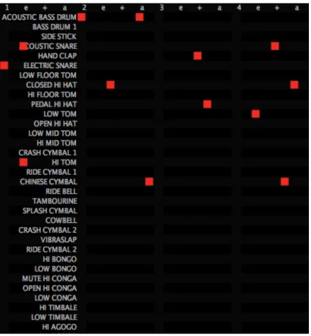
A user will be able to input a rhythm through the aid of a Drum Machine, which is a small application that is capable of playing and creating rhythms, which can then be converted into nodes. The Drum Machine’s musical timeline is represented by a vertical line that travels from left to right on the screen, when the line comes into contact with a note, that note is played. It should be noted however that the tempo (which is the speed of the musical timeline) does not have any influence on the rhythm itself, and is a direct specification of the Drum Machine component.
3.1. A Percussion Graph 15
Figure 3.2: The NetLogo Drum Machine
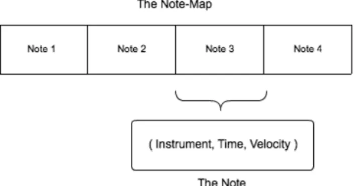
For each node, the rhythm is represented by a note-map or beat-map (see Figure 3.3), which is a list of all the notes in the drum machine. Each note consists of a triple that are the representations of the Instrument, the Time and the Velocity.
• The Instrument to be played, is represented by an Integer that corresponds to a specific instrument code.
• The Time which an instrument is played, is represented by an Integer that corre-sponds to a specific play time code.
• The Velocity that an instrument is played, is represented by an Integer that varies between 0 and 100. For the purpose of this experiment velocity only has two states, played (value is equal to 100) or not played (value is equal to 0).
So in conclusion what should be retained when discussing the Node is that it repre-sents a percussion rhythm, which internally is a note-map. A note-map is a drum pattern, like the one represented in Figure 3.2, and contains the information of the possible states (playing and non playing) of all the notes that the drum machine component is capable of offering.
16 CHAPTER 3. PERCUSSION GRAPHS
Figure 3.3: The Note-Map is the system’s representation of a rhythm
3.1.2
The Connection - The Directed Edge
The Connection is a sequence of percussion rhythms. This sequence can be represented as a list of note-maps (see Figure 3.4) and will contain various rhythms which will be played in order of input.
Figure 3.4: A Note-Map Sequence
A connection will start out empty initially, and will need to be filled with note-maps by an auxiliary function, which in the case of this research is done through our optimization processes.
3.2
Automated Connection - Generating Rhythms for the
Directed Edge
In a percussion graph there are no restrictions regarding the association between the graph components and percussion rhythms: a node can be associated with any kind of percus-sion rhythm and an edge can be associated with any possible sequence of percuspercus-sion rhythms.
For this research we envisioned a particular type of percussion graph, where each edge would be interpreted as a progressive transformation between two rhythms. What
3.2. Automated Connection - Generating Rhythms for the Directed Edge 17
this means is, if there is a directed edge between two nodes, it symbolizes the progres-sive transformation of the edge’s origin node into the edge’s end node. Which of course is something that could be done manually, but for the purpose of this work would be pointless. Instead, given the nodes’ respective rhythm’s and also the edges associated with them, the edges musical elements can be automatically generated through an op-timization process, where the sequence of percussion rhythms is the trace left by these optimization processes, which represent the progressive rhythm transformation from the edge start node until reaching the edge end node.
In order to guide the optimization process we will have to define an objective function that will rank a rhythm in terms of how similar it is relatively to another rhythm (which is our goal). The objective function will always be the same for each optimization process.
Figure 3.5: The Optimization Process
We also needed to define a way to stop the algorithm and we came up with two meth-ods:
• The Natural Stop Condition: Stops the optimization process once the objective function gives any generated rhythm a value of X or more, X being defined by the user. This gives the user liberty to stop the process when a rhythm’s similarity is sufficiently near the goal rhythm, and does not necessarily have to be a full exact equivalent.
• Sequence Length Stop Condition: Stops the optimization process based on the size of the sequence. This is useful in case an optimization process stalls or, is simply
18 CHAPTER 3. PERCUSSION GRAPHS
taking to long to reach the Natural Stop Condition. In a way, this stop condition is a fail safe, in case the first stop condition is never achieved.
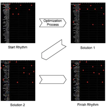
The sequence of rhythms which are obtained through the optimization processes will also be independent of which algorithm was used. We call these sequences Objective Maps, which are the consecutive solutions that are returned by our optimization processes. What this means is that, during the optimization process, an algorithm will progressively return solutions which will be kept by our objective map. These solutions will heavily vary depending on which algorithm was chosen, what the starting and ending rhythm was and a luck factor (or generative randomness).
Figure 3.5 shows a typical optimization process and its iterative solutions, note that for this particular example each iteration, the generated rhythms get relatively closer in similarity to the objective rhythm.
3.3
The Objective Function: Measuring the Rhythms
Sim-ilarity
The main role of the Objective Function is to evaluate any rhythm relatively to an objective rhythm.
For this we need to determine the similarity between one rhythm relatively to another rhythm (rhythms are note-maps). The Objective Function is described in Figure 3.6.
fobj(gen) = Similar(gen, obj)
Figure 3.6: The Objective Function
3.3.1
Measuring Rhythm Similarity
We think that they are two main component aspects for measuring similarity between any two rhythms. The first one being the number of active notes between the two note-maps, independently of the nature of the active notes. The second aspect being the similarity between the active notes of both rhythms. For that we’ll take into account the number of coincident active notes, however we also take into account that it is important to keep track of notes that are only coincident in time or instrument.
The Similarity Function (Figure 3.7) is the weighted sum of the length similarity and the position similarity, thus giving the liberty to change their relative importance.
The Similarity function value is a function that ranges from 1 to 10 (10 being that two rhythms are exactly the same) and their relative importance of the Similarity by length and
3.3. The Objective Function: Measuring the Rhythms Similarity 19
Similar(r1, r2) = Siml(r1, r2) × Lw Lw + N Ow +
Simn(r1, r2) × N Ow
Lw + N Ow
Figure 3.7: The Similar Function
position is given respectively by Lw and NOw. We experimented with these similarity weights and the best results obtained was simply giving the length a slightly lower weight (40-60 in favor of position) then the position weight, these values are the default weights.
Length Similarity
The term length refers to the number of notes that are played within a single note-map, for example if a rhythm has X playing notes the length will be X. The length similarity between any two rhythms will only depend on their lengths absolute difference as depicted in Figure 3.8. The farther away their lengths the lower the score.
Siml(r1, r2) = 10 ×
1
(|(length(r2) − length(r1)| + 1)
Figure 3.8: The Length Similarity Function
The Length Similarity can be analyzed in Figure 3.9, and shows how rigorous this function can be: the score is immediately halved once the length difference is 1.
Figure 3.9: The Variation of the Length Similarity, given the absolute difference between rhythms’ length
20 CHAPTER 3. PERCUSSION GRAPHS
Notes’ Similarity
The Notes’ Similarity evaluation will compare the nature of the active notes between one rhythm (r1) and a target rhythm (r2), thus it is a measure of how similar Rhythm 1 is to Rhythm 2. As we stated earlier in section 3.3.1, this measure will consider three aspects: Common Instruments, Common Times and Common Notes.
• Common Instruments ( I ): The number of distinct instruments that are played in both rhythms. Note that, if Rhyhtm 1 has two active notes that play maracas and Rhythm 2 only has one active note with that instrument, that instrument will only be counted once.
• Common Times ( T ): The number of distinct times that are played in both rhythms. Repeated active notes with the same time, will be counted in the same fashion as in the Common Instruments.
• Common Notes ( T ): The number of active notes that appear in both Rhythms.x
Each of these aspects will correspond to a respective function: I(r1,r2), T(r1,r2) and N(r1,r2). The Similarity function will be normalization of the weighted sum of these three functions and again will be a value between 1 and 10, as depicted in Figure 3.10.
Simn(r1, r2) = 10 ×
I(r1, r2) × Iw + T (r1, r2) × T w + N (r1, r2) × N w numI(r2) × Iw + numT (r2) × T w + length(r2) × N w
Figure 3.10: The Notes’ Similarity Evaluation
Its clear that the weight of the Common Note similarity should be significantly higher than the other two weights, and that both Common Instrument and Common Time should have an equivalent importance. By default we have chosen the value of 9 for the Common Note weight and the value of 1 for the Common Instrument and Common Time weights.
In order to normalize the function it was necessary to calculate the maximum possible value for the weighted sum (the numerator component of the formula). The maximum value is obtained when the first rhythm is exactly the same as the second rhythm. Note that we have to calculate the similarity of the first rhythm relatively to the second rhythm. Therefore, I(r1,r2) = numI(r2), T(r1,r2) = numT(r2) and N(r1,r2) = length(r2), where numI(r2) and numT(r2) corresponds respectively to the number of distinct Instruments and Times played in r2.
Illustration of the Similarity Calculation
We will illustrate the similarity function using as an example the two rhythms depicted in Figure 3.11.
3.3. The Objective Function: Measuring the Rhythms Similarity 21
Figure 3.11: The Played Notes of Rhythm r1 and Rhythm r2
We will begin by calculating the length similarity, given that r1has four played notes and r2 has three played notes (length(r1) = 4 and length(r2) = 3), and following for-mula 3.8 we obtain the results depicted in Figure 3.12.
Siml(r1, r2) = 10 ×
1
(|(3 − 4| + 1) = 5
Figure 3.12: The result of Length Similarity between r1 & r2
After the length similarity calculation we pass onto the notes’ similarity calculation. The intermediate calculations are:
• I(r1,r2) = 1, because there is only one common instrument between r1 & r2 (Instru-ment 1).
• T(r1,r2) = 2, because there are 2 common times between both rhythms (Time 2 & 4).
• N(r1,r2) = 2, because there are 2 notes ( [1,2] & [1,4] ) that belong to both rhythms. • To calculate the normalizing factor, we need to determine the length (length(r2) = 3), the number of distinctive instruments (numI(r2) = 2) and the number of distinc-tive times (numT(r2) = 3).
Following formula 3.10 and given the default weights (Nw = 9 & Tw = Iw = 1) we obtain the results in Figure 3.13
Simn(r1, r2) = 10 ×
1 × 1 + 2 × 1 + 2 × 9 2 × 1 + 3 × 1 + 3 × 9 = 6.4
Figure 3.13: Notes’ Similarity value of r1 relatively to r2
Finally, in order to calculate the global similarity of r1 relatively to r2, we will use the default values for the weight parameters(Lw = 0.4 & NOw = 0.6) and following for-mula 3.7 we obtain the result in Figure 3.14
22 CHAPTER 3. PERCUSSION GRAPHS
Similar(r1, r2) = 5 × 0.4 0.4 + 0.6 +
6.4 × 0.6
0.4 + 0.6 = 5.84
Figure 3.14: The Similar Function result of r1 relatively to r2.
3.4
Optimization Processes
3.4.1
Genetic Evolution Process
The Genetic Evolution Algorithm is a search algorithm inspired by the natural process of evolution [Dar58]. The algorithm consists of creating populations of candidate solutions (called chromosomes) to the optimization problem and applying natural evolutionary tac-tics, such as crossovers, mutations and selections. The algorithm starts out by creating a population of randomized individuals who are then ranked by a fitness function. De-pending on their rank the individual might be selected or not for the breeding phase. The breeding phase will create a new generation population, consequently re-iterating the ranking, selection and breeding phase on this new generation. This is done until the optimum solution is found.
The Genetic Evolution algorithm was the first optimization process to be developed for this research. According to Mitchell M. [Mit98] there are various ways to approach genetic algorithms (GA’s), but the most common approach is by separating the algorithm in 3 phases:
• Fitness Application • Selection
• Crossover and Mutation
The idea of the genetic model is to create a population of individuals who will then be ranked by a fitness function. Taking into consideration each individuals rank, a selection method is called. This method will pick a number of individuals (the individuals picked depend heavily on the selection type) that will go into the breeding phase. In the breed-ing phase two individuals will suffer a crossover and might have a chance of mutatbreed-ing, creating new individuals. This can be done Nth number of times from selection to breed-ing until reachbreed-ing the population cap, whereas from there, each individual will be ranked again by the fitness function.
Implementation Specifics
Each Chromosome (or Individual) will be a note-map and the fitness will be our objective function (as defined in 3.6). The best ranked chromosome of each generation will be kept within the objective map.
3.4. Optimization Processes 23
Figure 3.15: The Genetic Algorithm Evolution
We also needed a population to kickstart the genetic process. This process would need to take into consideration the starting node’s rhythm, so we created a ”special” mutation function, one that could mutate the starter rhythm, but still keep most of its elements in-tact. This starter mutation would then run N times (N being the population size), creating a population pool that could be used by the genetic algorithm.
Finally we needed to define the algorithms stop conditions. Because of the unpre-dictability of the natural stop condition, which by default is set to 10, we also defined a sequence length stop condition. By default the sequence length stop is set to 75 genera-tions which means that, after 75 solugenera-tions were generated, and no solution has satisfied the natural stop condition, the algorithm stops and returns all the solutions that were obtained until generation 75.
When we were discussing the implementation of the genetic algorithm within our system, we pondered on the idea of implementing the genetic model ourselves, however a better solution was to just use an available working API. JGAP[Mef] included all of the options we needed to make this genetic model work, except a few minor exceptions.
Selection
Selection algorithms choose which chromosomes from a population are to breed for the next generation. If a particular chromosome is fitter than the other, doesn’t necessarily mean it will be chosen. Depending on the algorithm the fitter chromosome might have a bigger or the same chance to breed than the less fit chromosome. But most of the time the
24 CHAPTER 3. PERCUSSION GRAPHS
probability is always in favor of the fittest chromosome.
We ended picking the Roulette Selection method as it favors higher ranked chromo-somes but not always. The Roulette Selection is a fitness-proportionate methodology[Mit98], where the fitness values of each chromosome influence the probability of selection. In the case of the roulette, each chromosome is assigned a slice of a circular ”roulette wheel”, where the size of the slice is proportional to the fitness that was given to each chromo-some. The roulette is then spun N times (N being the number of the population) and the chromosome chosen by the ”wheel’s marker” is selected to breed.
1. Sum the total expected value of the individual’s fitness, and call this value T.
2. Repeat N times:
(a) Choose a random integer r between 0 and T.
(b) Loop through the individuals in the population, summing the expected values, until sum is greater than or equal to r. The individual whose expected value puts the sum over this limit is the one selected.
Figure 3.16: Representation of the Roulette Selection
Elitism
The Evolutionary process also uses elitism. Elitism forces the genetic algorithm to keep the best-ranked N number of chromosomes from one generation and automatically move them towards the next generation[Mit98]. This helps keep the population in-check and the chromosomes from worsening with each new generation. However Elitism has the side-effect of staling a population creating very similar chromosomes if left unchecked, so it is always important to keep the elitist population low compared to the whole.
3.4. Optimization Processes 25
For this research we decided to apply elitism to 25% of the population, which means that in a population of 500 chromosomes, the best 125 chromosomes would be picked for the next generation. However this should not be confused with the solution that is picked for the objective map, the solution is always one and only one chromosome, which is the best out of all the chromosomes of one generation (which in case of a tie is randomly picked).
During some experiments we did try to forgo elitism, however it proved to be difficult for the algorithm to converge towards it’s goal, as it was always struggling with un-fit and fit solutions until stabilizing into a regular score after multiple generations. Musically, without elitism the sounds within the middle generations were always chaotic with new variations always occurring, however most of the time these variations were tame, with three to four notes shifting from one place to another.
Crossover
Once the individuals have been chosen, its time to apply the crossover. The crossover is a generic concept which consists of mixing the contents of two chromosomes as a means of generating two new chromosomes. Each chromosome (in this case the note-map) chosen for crossover is split in two, where the location of the cut is defined by a cutting point, subsequently each half is then joined with the other chromosome’s halves. This will create two new individuals, each of them containing half of their parents genes. The cutting point of an individual’s chromosome can be random or defined, in this case it is defined at the middle of a chromosome.
Figure 3.17: Representation of the Crossover Method
Figure 3.17 exemplifies how the crossover is applied within our system. The lines rep-resent cutting points made upon each of the chromosomes. The results obtained through
26 CHAPTER 3. PERCUSSION GRAPHS
this process still have a probability of suffering mutation, but afterwards are added to the new population.
Mutation
Mutation is a simple random percentage factor applied to a new-bred individual, which affects it’s chromosome in a minor way[Mit98], such as changing a random 1 to 0 (or vice versa), or remove/add a bit for example.
For this experiment our standard mutation is simply the act of transforming a random playing note into a non-playing note or vice versa. The generic mutation function can influence a note in the following ways:
• Play: If that note is currently silent.
• Silent: If that note is currently playing.
In reality what it is doing is setting the Velocity to either 0 or to 100, which affects the notes being played, in this case its sonority.
However, it was necessary to create two types methods, on how this standard mutation algorithm would be applied onto our chromosomes. We needed one method that would kickstart the genetic process (as mentioned earlier), and another method that would be used during the evolutionary process itself. Its important to note that both of these meth-ods would apply our standard mutation, although in different ways.
Initial Population Kickstart This method will take a note-map and select a random number between 0 and N (by default N = 5). For N times the function will choose one random position from the note-map and modify that note using the standard mutation function.
For the genetic algorithm specifically, this is done X times on the origin note-map, so as to create our initial population. This step is necessary to create a diversified initial population, so the chromosomes don’t stale and the genetic process can come up with more diversified solutions. Usually the population initialization is randomized[Mit98], however in the specific case of this work it wouldn’t make sense, because we want to keep some attributes of the origin note-map and not discard it completely.
It also should be noted that this method will work on any note-map type, and will in fact be used for some of our other optimization processes.
Evolutionary Method Mutation This method unlike the kickstart method, applies a probability of applying the standard mutation to every note during the evolutionary pro-cess. What this means is, that a note would have the probability of 1 in N chances of being
3.4. Optimization Processes 27
switched from play to silent or silent to play. By default N is set to 1000, so on average there is a probability that one within a 1000 notes will be mutated.
Also it is important to emphasize that this method is used during the evolutionary process itself.
3.4.2
Hill Climbing Process
The Hill Climbing Process uses a local search algorithm[MF04] (one of the various hill-climbing techniques) which focuses its search within a local neighborhood. The Local Search Algorithm goes as follows[MF04]:
1. Pick a solution from the search space and evaluate its merit. Define this as the current solution.
2. Apply a transformation to the current solution to generate a new solution and eval-uate its merit.
3. If the new solution is better than the current solution then exchange it with the current solution; otherwise discard the new solution.
4. Repeat step 2 and 3 until the objective function gives a value that is at least equal to the user defined, natural stop condition (this step is specific to our research).
Figure 3.18: The Hill Climbing Process
First we had to define the neighborhood and the solution acceptance criteria. The neighborhood function was going to be variations of the last best solution or starting node (to kickstart the algorithm). Our Initial Population Kickstart method, which we created for our genetic algorithm component served perfectly well for our neighborhood function. The criteria for inserting a solution into our objective map was set to ”once the solution
28 CHAPTER 3. PERCUSSION GRAPHS
improves”. If a new generated solution satisfied this criteria, it would then be added to the objective map.
The process will always iterate over the last best note-map obtained, then apply the neighborhood function to it and finally rank it using the objective function, over and over until a better note-map is found. The iteration will run until a note-map reaches or passes the natural stop condition threshold (by default is set to 10). For this particular optimization process we did not set any length sequence stop condition, as it wasn’t really necessary, because the algorithm worked fairly well with only the natural stop condition. So in theory, once the optimization process has finished, we can expect a song that never repeats itself, thanks to the intrinsic nature of this algorithm (by only adding note-maps that are improvements of the precedent one). But on the other hand songs are much shorter, because their are less solutions entering the objective map, at least when compared to its genetic counterpart.
3.4.3
Stochastic Hill Climbing Process
The Stochastic Hill Climber is a modification of the Hill Climbing process, where the largest difference lies within the acceptance criteria. While the normal Hill Climbing method focuses on a more opportunistic approach of ”Keep solution immediately, if best”, the Stochastic’s acceptance criteria is based on a probabilistic nature, where the rule of moving from a current solution vc to a new solution vn is based on a probability. The
probabilistic formula for accepting a new solution focuses on maximizing the objective evaluation function[MF04], which means that a better ranked solution will garner a better chance of being picked than a lower ranked solution.
p = 1
1 + eeval(vc)−eval(vn)T
Figure 3.19: The Probability of Acceptance
Analyzing Figure 3.19 the probability of acceptance depends heavily on the difference of merit between the score obtained by the last solution (vc) and the score of the new
solution (vn) and of an additional parameter T. The T parameter influences the sway of
the acceptance rate, for example the higher the T value is, the better the chance that a worse solution has of being accepted, the lower the T value the lower the chances are of a worse solution being accepted. The challenge of this algorithm is to find a T value ”sweet spot” so to say, one that does not overcompensate worse solutions but also does not completely shut them down (if that were the case we’d have a normal Hill Climbing Algorithm).
3.4. Optimization Processes 29
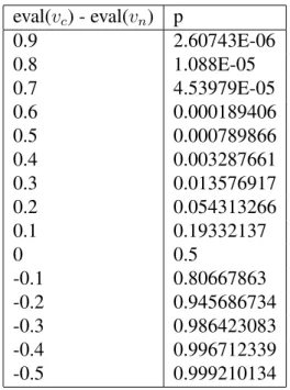
To come up with a good T value we started out by randomly tweaking it and analyzing the objective maps solutions. We found that a T value between 0 and 0.1 were garnering the best results. So using an Excel spreadsheet we found a pretty good value of T = 0.07.
eval(vc) - eval(vn) p 0.9 2.60743E-06 0.8 1.088E-05 0.7 4.53979E-05 0.6 0.000189406 0.5 0.000789866 0.4 0.003287661 0.3 0.013576917 0.2 0.054313266 0.1 0.19332137 0 0.5 -0.1 0.80667863 -0.2 0.945686734 -0.3 0.986423083 -0.4 0.996712339 -0.5 0.999210134
Table 3.1: Value of P with T = 0.07
However we did have another problem, which was of repetitiveness. When we exper-imented the algorithm we saw that a lot of the times our objective map would be flooded with the same ranked note-maps over and over, because the acceptance rate of two equiva-lent note-maps was at 50%, which by analyzing Table 3.1 we can clearly see this in effect, when eval(vc) - eval(vn) = 0. So to circumvent this we decided that if no changes were
made to the note-map’s rank the probability would be immediately ignored and pass to another solution. This allowed us to eliminate the repetitiveness of the final solution just like the normal hill climber.
The idea behind the stochastic hill climber is about creating a regressive possibility, which is counter to the normal hill climbing’s ”always best” kind of nature. This will create a more unpredictable song output, because the solution isn’t merely trying to get towards its goal.
3.4.4
Optimization Filters
During the prototyping of the application we realized that a lot of the solutions that were returned by, most specifically the genetic optimization, contained a lot of repetitious pat-terns and very long objective maps, something that could saturate the listener from a overabundance of generated content. This, of course, was mostly due to the fact that we were using elitism in the genetic process. Although this was not the only reason, we also
30 CHAPTER 3. PERCUSSION GRAPHS
wanted to give the user some simple editing tools, such as discarding unwanted parts of a solution.
Filters are methods of shortening the optimization solutions, which have probably grown too large for it to be usable. A filter will take care of shortening a solution by eliminating note-maps according to a user selected specification. For the purpose of this research we created 3 types of Filters:
• The Point to Point Cut
• The Rank Cut
• The Repetition Cut
Filters aren’t mutually exclusive, meaning that if a user applies a Point to Point Cut he can also apply a Fitness or Repetition Cut if he so chooses. However, there are filters that do not make sense on certain optimization processes such as applying the repetition cut on a hill climbing solution, for example.
The Point to Point Cut
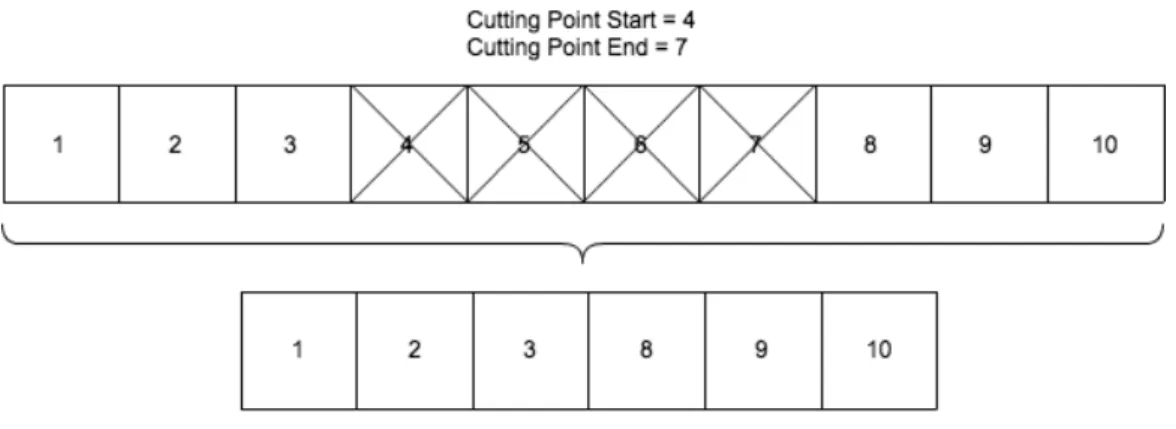
The Point to Point Cut is a filter method that cuts the N note-maps between a position X and a position Y of an objective map (Figure 3.20). This filter takes into consideration the position of a note-map within the objective map and will cut all note-maps whose position is equal or higher to X and equal or lower than Y. This filter should be used mostly as a form of editing tool, which will cut unwanted parts of the song.
Figure 3.20: The Point to Point Cut Filter
The Rank Cut
The Rank Cut is another type of filter, which consists of eliminating all of the note-maps from an objective map, whose rank are not within a user specified interval. For example