Description and modelling of thermophysical properties and excess of eutetic mixtures

Universidade de Aveiro C/ Currículo Sim Data 07/11/2018

CARACTERIZAÇÃO E MODELAÇÃO DE PROPRIEDADES TERMOFÍSICAS E DE EXCESSO DE MISTURAS EUTÉTICAS

João Miguel Lopes Costa

Dissertação de mestrado em Mestrado Integrado em Engenharia Química, apresentada ao Departamento de Química da Universidade de Aveiro, sob orientação de Dr. Pedro Jorge Marques Carvalho e coorientação de Prof. Dr. João Manuel da Costa Araújo Pereira Coutinho.

i

JOÃO MIGUEL LOPES COSTA

CARACTERIZAÇÃO E MODELAÇÃO DE PROPRIEDADES TERMOFÍSICAS E DE EXCESSO DE MISTURAS EUTÉTICAS DESCRIPTION AND MODELLING OF THERMOPHYSICAL PROPERTIES AND EXCESS OF EUTETIC MIXTURES

JOÃO MIGUEL LOPES COSTA

CARACTERIZAÇÃO E MODELAÇÃO DE PROPRIEDADES TERMOFÍSICAS E DE EXCESSO DE MISTURAS

EUTÉTICAS

DESCRIPTION AND MODELLING OF THERMOPHYSICAL PROPERTIES AND EXCESS OF EUTETIC MIXTURES

Dissertação apresentada à Universidade de Aveiro para cumprimento dos requisitos necessários à obtenção do grau de Mestre em Engenharia Química, realizada sob a orientação científica do Doutor Pedro Jorge Marques Carvalho, investigador auxiliar do Departamento de Química da Universidade de Aveiro (CICECO) e co-orientação do Doutor Professor João Manuel da Costa Araújo Pereira Coutinho, Professor Catedrático do Departamento de Química da Universidade de Aveiro.

o júri

presidente Professor Dr. Carlo Manuel Silva

Professor associado do departamento de química da Universidade de Aveiro

Professor Dr. Abel Ferreira

Professor assistente do departamento de engenharia química da Universidade de Coimbra

Professor Dr. Pedro Jorge Marques de Carvalho

I would also like to express an exceptional gratitude to Professor Dr. João Coutinho for receiving me in his unique research group, Path, for all these last four years and also giving me the opportunity to live a new experience working abroad.

I would be extremely ungrateful if I did not thank to all the Path members for all the support and motivation.

I would like to dedicate some words of acknowledgment to Liliana Silva that always helped me in everything that needed and to Emanuel Crespo that also gave me two helping hands every time I was stuck in soft-SAFT.

A very special thank to Dr. Pedro Carvalho for not giving up on me, for enduring my anxious behavior, for all the support and attention, for heling me at abusive off scheduled hours and for bearing my doubts in this work and in myself and for almost everything else because without him this work would not exist and I would never get the master degree in chemical engineering, i cannot promise I will be ever be good at it but he did the possible and the impossible to make it happen.

It is important for me to appreciate my friends for being my friends, for keep motivating me when I was down and for the contribute they gave to the development of this work.

At last, but definitely not least, I like to thank to my parents that sponsor my education.

palavras-chave Solventes Eutéticos Profundos, Viscosidade, Densidade, Equilíbrio Vapor-Líquidos, Equações de Estado, soft-SAFT, Alta Pressão

impacto ambiental, têm projetado estes solventes alternativos para um grande número de aplicações, nomeadamente na eletroquímica, na catálise, na síntese orgânica, em processos de dissolução e extração e na dessulfurização de combustíveis. Os DES formam-se de uma mistura eutética de um dador de ponte de hidrogénio (HBD) e um recetor de pontes de hidrogénio (HBA). Devido ao seu potêncial e às enúmeras aplicações propostas, a sua caracterização físico-química torna-se extremamente relevante quando se imagina a sua introdução em processos industriais. Este trabalho é focado na formulação das misturas eutécticas compostas por [Ch]Cl + [EG], [Ch]Cl + [Gly] e [Ch]Cl + Ureia, e na sua caraterização termofísica, nomeadamente viscosidade, densidade e pontos de ebulição numa gama de temperatura entre 283.15 K e 363.15 K e a pressões entre 0.1 e 100MPa. Os dados experimentais foram posteriormente modelados usando a equação de estado (EoS) soft-SAFT; uma EoS capaz de ter em consideração a associação existente entre os componentes do DES e que consegue descrever a sua não idealidade em fase liquida. O desenvolvimento da soft-SAFT permitiu propor um novo esquema associativo e novos parâmetros moléculares para a ureia.

keywords Deep Eutectic Solvents, Viscosity, Density, Vapor-Liquid Equilibrium, Equation of State, soft-SAFT, High Pressure

projecting them as alternative solvents for a large number of applications, like catalysis, organic synthesis, dissolution and extraction processes, electrochemistry, material chemistry and desulfurization of fuels. DES are formed by an eutectic mixture of a hydrogen bond donor (HBD) and a hydrogen bond acceptor (HBA). Owing to their promising applications, their physicochemical characterization, aiming at their use on industrial processes, stands highly relevant.

This work focus on the formulation of eutectic mixtures, composed of [Ch]Cl + [EG], [Ch]Cl + [Gly] e [Ch]Cl + Ureia, and their thermophysical characterization, namely viscosity, density and boiling temperatures, at a wide range of temperatures (283 to 363 K) and pressures (0.05 to 100 MPa). The experimental data was further modeled using the soft-SAFT equation of state (EoS); an advance EoS able to explicitly account for the association between the DES constituents and shown to be able to describe the nonideality of the liquid phase. The soft-SAFT development allowed to propose new association schemes and molecular parameters for urea.

i

LIST OF FIGURES ... III LIST OF TABLES ... V NOMENCLATURE ... VI

1 INTRODUCTION ... 1

1.1. GENERAL CONTEXT ... 2

1.2. SCOPE AND OBJECTIVES ... 7

2 MODEL AND EXPERIMENTAL APPARATUS ... 9

2.1 SOFT-SAFTEQUATION OF STATE ... 10

2.2 HIGH PRESSURE DENSITY ... 14

2.3 HIGH PRESSURE VISCOSITY ... 16

2.4 ISOBARIC EBULLIOMETER... 22

3 MATERIALS ... 25

3.1 EUTETIC SYSTEMS ... 26

3.2 SAMPLES PREPARATION ... 26

4 EXPERIMENTAL RESULTS ... 29

4.1 DESHIGH PRESSURE DENSITY ... 30

4.2 DESHIGH PRESSURE VISCOSITY ... 32

4.3 VAPOR –LIQUID EQUILIBRIUM ... 36

5 MODELLING ... 37

5.1 STRATEGY TO MODEL THE EXPERIMENTAL DATA ... 38

5.2 DENSITY MODELLING RESULTS ... 40

5.3 VISCOSITY MODELING RESULTS ... 43

6 CONCLUSION ... 48

7 FINAL REMARKS AND FUTURE WORK... 49

8 REFERENCES ... 50

APPENDIX A – EXPERIMENTAL RESULTS ... 59

iii

Figure 1.1 Scheme that represents the difference between the eutectic point of an ideal

mixture and a DES. ... 4

Figure 2.1 Schematic representation of the physical foundation of SAFT-type equations.

... 10

Figure 2.2 Schematic representation of the soft-SAFT molecular parameters. ... 11

Figure 2.3 Schematic representation of the apparatus of the DMA-HPM measuring cell

with the movable piston. ... 15

Figure 2.4 Julabo F25-HE thermostatic bath (left) and Automated pressure generator

(right). ... 17

Figure 2.5 Scheme that represents the coils around the fluid tube. ... 18

Figure 2.6 Measuring cell (left) and monitoring setup (rigth) composed by an Agilent

34970A thermometer, Agilent 33220A wave generator and Agilent U2352A data

acquisition. ... 19

Figure 2.7 From the left to the right, the TRIVAC D8B vacuum pump with the cold trap

TK 4-8 and the Pirani vacuum measurer. ... 20

Figure 2.8 Vibrating wire viscometer with a manual pressure generator and the separation

funnel from which the sample is introduced. ... 21

Figure 2.9 Schematic representation of the isochoric ebulliometer, figure taken from

Stuckenholz et al.

. ... 24

Figure 4.1 Density percentage relative deviation between the experimental and literature

data. Data from (left) Shahbaz et al.

in orange and red, Mjalli et al.

in

green, grey and Yadav et al.

in yellow and blue, (right) Leron et al.

. . 31

Figure 4.2 Density as function of pressure and temperature for [Ch]Cl + EG, [Ch]Cl + Gly

and [Ch]Cl + Urea. ... 32

Figure 4.3 Viscosity as function of temperature for the systems [Ch]Cl + EG, [Ch]Cl +

Gly and [Ch]Cl + Urea, at atmospheric pressure. viscosity data was obtained using the

○ SVM3000, ■ vibrating wire, ♦ falling body, ▲ from D’Agostino et al.

_{, ♦ from}

Yadav et al.

and ● from Abbott et al.

. ... 34

Figure 4.4 Viscosity as function of pressure and temperature for the [Ch]Cl + EG, [Ch]Cl

+ Gly and [Ch]Cl + Urea mixtures. ... 35

Figure 4.5 Boiling temperatures as function of the EG mole fraction for the mixture of

Urea with ethylene glycol at 0.1 MPa and 0.07 MPa. ... 36

Figure 5.1 Schematic representation of the [Ch]Cl, EG, Gly and Urea molecules with the

respective interaction sites, each letter represent a different association site and the

color redand blue represent the negative or positive character of the sites, respectively.

... 40

Figure 5.2 VLE as function of composition and pressure for the urea + EG system. The

solid lines represent the soft-SAFT EoS description. ... 41

Figure 5.3 Density as a function of temperature and pressure for the three DES studied

plus the mixture urea with ethylene glycol. The solid lines represent the soft-SAFT

results. ... 43

iv

found in the literature ... 45

Figure 5.5 Viscosity as function of temperature and pressure for the three DES evaluated.

The solid lines represent the soft-SAFT EoS description. ... 46

Figure B.1.

Density as a function of temperature and pressure the choline chloride with

urea, the solid lines represent the soft-SAFT prediction while the symbols are the

experimental

data

shown

above.

………..70

Figure B.2. Density as a function of temperature at atmospheric pressure for the mixture

Urea with ethylene glycol, the solid lines represent the soft-SAFT prediction while the

symbols are the experimental data shown above. ... 71

Figure B.3. Viscosity as a function of temperature and pressure for pure ethylene glycol,

the solid lines represent the soft-SAFT prediction while the symbols are the

experimental data found in the literature. ... 72

Figure B.4. Viscosity as a function of temperature at atmospheric pressure for pure

glycerol, the solid lines represent the soft-SAFT prediction while the symbols are the

experimental data found in the literature. ... 73

Figure B.5. Viscosity as a function of temperature at atmospheric pressure for the eutectic

solvents choline chloride with ethylene glycol and with glycerol, the solid lines

represent the soft-SAFT prediction while the symbols are the experimental data found

in the literature. ... 74

Figure B.6. Boiling points of the mixture urea with ethylene glycol in function of the

compositions of ethylene glycol at atmospheric pressure, the solid line ae the

soft-SAFT prediction while the symbols are the experimental data ... 75

v

mass fraction purity, and supplier of the compounds studied in this work. ... 27

Table 3.2.Masses of the compounds and choline chloride mole fraction used in the

preparation of the studied mixtures. The mixtures of this table were used to study the

viscosity behavior. ... 28

Table 3.3.Masses of the compounds and choline chloride mole fraction used in the

preparation of the studied mixtures. The mixtures of this table were used to study the

density behavior. ... 28

Table 5.1.soft-SAFT molecular and viscosity parameters gathered from literature

and optimized in this work. ... 47

Table 5.2.soft-SAFT binary interaction parameters used for each system. ... 47

Table A 1 Density as function of pressure and temperature for the [Ch]Cl + EG deep

eutectic

mixture.

………..60

Table A 2 Density as function of pressure and temperature for the [Ch]Cl + Gly deep

eutectic mixture ... 61

Table A 3 Density as function of pressure and temperature for the [Ch]Cl + Urea deep

eutectic mixture ... 62

Table A 4 Density as function of pressure and temperature for the [Ch]Cl + EG mixture

with 2:3 molar ratio. ... 63

Table A 5 Density as function of pressure and temperature for the [Ch]Cl + EG mixture

with 3:7 molar ratio. ... 64

Table A 6 Density as function of temperature for the Urea + EG mixture at atmospheric

pressure... 65

Table A 7 Viscosity as function of temperature and pressure for pure ethylene glycol

found in the literature

... Erro! Marcador não definido.

Table A 8 Viscosity as function of temperature and pressure for [Ch]Cl + EG eutectic

mixture. Found in the literature

... Erro! Marcador não definido.

Table A 9 Viscosity as function of temperature for glycerol, at 0.1 MPa. ... 66

Table A 10 Viscosity as function of temperature and pressure for [Ch]Cl + Urea eutectic

mixture. ... 66

Table A 11 Viscosity as function of temperature and pressure for the [Ch]Cl + Gly eutectic

mixture. ... 67

Table A 12 Boiling temperatures as function of the composition of ethylene glycol for the

Urea + EG mixture, at 0.07 MPa. ... 67

Table A 13 Boiling temperatures as function of the composition of ethylene glycol for the

Urea + EG mixture, at 0.1 MPa. ... 68

Table B.1.Urea soft-SAFT EoS molecular parameters for the optimization attempts. . 70

Table B.2. soft-SAFT EoS viscosity parameters tested for ethylene glycol. ... 71

Table B.3. soft-SAFT EoS viscosity parameters tested for glycerol. ... 72

Table B.4. soft-SAFT EoS viscosity parameters tested for choline chloride. ... 73

vi

Nomenclature

Symbol Description of the symbol SI units

𝐴 Constant of calibration -

𝑎 Soft-SAFT total Helmotz energy 𝐽/mol

𝑎𝑎𝑠𝑠𝑜𝑐 Soft-SAFT association term 𝐽/mol

𝑎𝑐ℎ𝑎𝑖𝑛 Soft-SAFT chain association term 𝐽/mol

𝑎𝑖𝑑 Soft-SAFT total Helmotz energy in the ideal case 𝐽/mol

𝑎𝑝𝑜𝑙𝑎𝑟 Soft-SAFT polar term 𝐽/mol

𝑎𝑟𝑒𝑓 Soft-SAFT reference term 𝐽/mol

𝑎𝑟𝑒𝑠 Soft-SAFT residual term 𝐽/mol

𝐵𝑖 Soft-SAFT viscosity parameter of the substance i -

𝐵𝑚𝑖𝑥𝑡 Soft-SAFT viscosity parameter of the mixture -

𝑓 Frequency 𝐻𝑧

𝑓0 Resonance frequency in vacuum 𝐻𝑧

𝑓𝑏 Half-width of the resonance curve 𝐻𝑧

𝑓𝑟 Resonance Frequency 𝐻𝑧

𝑘𝐻𝐵 Soft-SAFT cross-association Volume Å3

𝐿𝑣 Soft-SAFT viscosity parameter Å

𝐿𝑣,𝑚𝑖𝑥𝑡 Soft-SAFT viscosity parameter of the mixture Å

𝑀𝑊 Molar weight 𝑘𝑔−1∙ 𝑚𝑜𝑙−1

𝑚 Soft-SAFT chain length -

𝑝 Pressure 𝑃𝑎

𝑝𝑠𝑎𝑡 _{Saturation pressure 𝑃𝑎}

𝑝𝑟𝑒𝑓 Reference pressure 𝑃𝑎

period Period 𝑠

R Constant of the ideal gases 𝐽 ∙ 𝐾−1_{∙ 𝑚𝑜𝑙}−1

𝑟 Radius 𝑚

vii

𝑇𝑟𝑒𝑓 Reference temperature 𝐾

𝑉1 Voltage 𝑣

𝑉2 Wire movement 𝐻𝑧−1

𝑥 Molar fraction of a liquid -

𝛼 Soft-SAFT viscosity parameter 𝐽 ∙ 𝑚3∙ 𝑚𝑜𝑙−1∙ 𝑘𝑔−1

𝛼𝑚𝑖𝑥𝑡 Soft-SAFT viscosity parameter of the mixture 𝐽 ∙ 𝑚3∙ 𝑚𝑜𝑙−1∙ 𝑘𝑔−1

𝛼𝑣𝑡 Coefficient of the thermal expansion 𝐾−1

𝛽 Additional mass of the fluid -

𝛽′ _{Damping due to fluid viscosity -}

𝛽𝑣𝑡 Coefficient of the thermal compressibility 𝑃𝑎−1

∆0 Logarithmic decrement of the wire in vacuum -

∆𝜌 Density variation 𝑘𝑔 ∙ 𝑚3

𝜀 Soft-SAFT dispersive energy 𝐾

𝜀𝐻𝐵 _{Soft-SAFT cross-association energy 𝐾}

𝜂 Viscosity 𝑃𝑎 ∙ 𝑠

Λ Amplitude -

𝜎 Diameter of a molecular sphere Å

𝜌 Density 𝑘𝑔 ∙ 𝑚3

1

2

1.1. General Context

Horizon 2020 is the biggest EU programme that encourages research and innovation promising breakthroughs, discoveries and world-firsts by taking great ideas from the lab to the market. In the working program of the horizon 2020 programme several goals on climate policies, aiming at the reduction of the carbon and solvent emissions, are proposed. The deadline of some of these goals such as the topics “Supporting the development of climate

policies to deliver on the Paris Agreement, through Integrated Assessment Models (IAMs)” and

“Climate change impacts in Europe”, just to name a few, have recently expired, with some of the proposed targets not being accomplished on time. Thus new regulations are going to be proposed with more challenging and demanding targets. On the other hand, the Registration, Evaluation, Authorization and Restriction of Chemicals (REACH), a regulator that improves the protection of human health and the environment through a better and earlier identification of the intrinsic properties of chemical substances, has over the years been restricting and controlling the use of organic solvents and protocols, to treat their before the release to the environment, aiming at reducing the environmental impact. All these political decisions have inspired researchers to develop alternatives to organic solvents.

Conventional industrial organic solvents are a source of pollution with direct impact on the ozone depletion, disruption of natural ecosystems and persistent bioaccumulation. These solvents are not only an environmental concern, but people are also further exposed to them on two different ways: inhalation or cutaneous contact and, in some cases, ingestions due to unintentional or accidental exposures. The exposure to solvents have substantial neurotoxic effect to central and peripheral nervous systems which can produce severe and irreversible toxic leukoencephalopathy, more known as white matter dementia[1]_.

Industries like painting[2]_{, construction}[3]_{, furniture finishing}[4]_{, metal degreasing and}

finishing[5]_{, mechanical and refrigeration systems maintenance}[6]_{, rubber}[7]_{, polymer}[8]_{, textile and}

leather[9] _{production rely on the use of organic compounds on their processes. Thus, searching}

for alternative solvents stands highly relevant on a near future.

In the last few decades, ionic liquids (ILs), a class of green solvents, have attracted the interest from both industry and academia. ILs consist on a salt whose ions are organized in such way that allows them to be in the liquid state bellow 100 ºC. The term “ionic liquid” was coined

3 for the first time back in 1914 by Paul Walden[10] _{for a mixture of ethylammonium nitrate, which}

was, at that time, proposed to be used as an alternative to nitroglycerin in explosives[11]_{. Only}

recently, studies on ionic liquid’s properties revealed the great potential of these compounds as an alternative for conventional solvents. The properties that make IL interesting as a solvent are: negligible vapor pressure, negligible flammability, thermal stability and highly solvating capacity either for polar and nonpolar compounds[12]–[15]_{. Other applications besides solvent action have}

been pointed to ILs, since they have been referenced to be used in lubricants[16]_{, deep}

desulfuration of diesel fuel[17]_{, thermal fluids}[18]_{, fuel cells}[19]_{, metal finishing}[20]_{, gas}

separations[21]_{, extractions}[22] _{of calcium from spiral microfluids}[23]_{, of styrene from}

ethylbenzene[24]_{, of verbascoside from Rehmannia root}[25]_{, of succinic acid from bio mass}[26] _and

recovery of Indium based on the combination of ionic liquid extractions with electrodeposition[27]

and liquid membranes[28]_{, just to name a few. Ionic liquids have been claimed as environmentally}

friendly since they are non-volatile (do not cause air pollution). Moreover, being composed of ions their simple combination allows one not only synthesize 106 _{different ionic liquids but to}

tune the solvent’s properties, like density, viscosity, surface tension or even biodegradability and toxicity for microorganisms, invertebrates and vertebrates, designing them for a specific and to be “environmental friendly”[29][30]–[32]_.

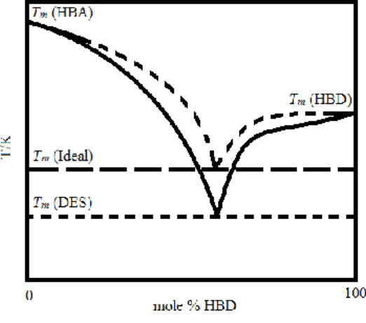
Another alternative to conventional solvents are deep eutectic solvents (DESs). The etymology of the word eutectic comes from the Greek word ευτηκτος, which mean easy to melt. The first person to use the term eutectic was the British physicist Frederic Guthrie in 1884. At that time this term was used to define “a lower temperature of liquefaction than that given by

any other proportion”. In a mixture, the interception of two solubility curves, which represents

the composition at the minimum melting temperature of the mixture, is called the eutectic point, as depicted in Figure 1.1. DESs are eutectic mixtures of two (or more) compounds, a hydrogen-bond donor (HBD) and an hydrogen bond acceptor (HBA), able to establish strong and highly complex hydrogen bonds, that due to those interactions present a significant melting temperature depression compared to the melting temperatures expected for an ideal system.

It is important to stress that there is still some misconception around the definition of DES. They are not novel compounds or pure substances neither a new type of ionic liquid (although, most DESs reported in the literature have an ionic liquid as HBA).[33] _{In fact, many mixtures are}

reported to be a DES but, if one evaluates their deviation to ideality, they are just common eutectic mixtures[33][34]_{. The majority of DESs reported in literature are composed by a}

4

quaternary ammonium halide salt, as a hydrogen bond acceptor (HBA), and a hydrogen-bond donor (HBD) that can vary from amides[35] _{(like urea and its derivatives), polyols and polyalcohols}

(like glycerol[36]_{, ethylene glycol}[37] _{or triethylene glycol}[38]_{), carboxylic acids (like oxalic}[39]_,

malonic[40] _{or glutaric acid}[41]_{) and even sugars (like D-fructose}[42]_{, D-glucose}[43] _{or xylitol}[44]_).

Figure 1.1Scheme representing the difference between the eutectic point of an ideal mixture and that of a DES.

Smith et al.[1] _{proposed a general formula to classify different DESs into four types,}

according to the nature of the DES constituents. The type I are characterized by a metal salt and an organic salt.[45] _{Type II consists of a mixture of hydrated metal halide with an organic salt, this}

type being suitable to industrial processes because of their low price and easy shipping since it is insensible to inherent air or moisture.

Using [Ch]Cl and a hydrogen bond donor, such as amides, carboxylic acids and alcohols one can form a type III DES[46]_{. The type III DES are composed by an organic salt and a HBD making}

this type of DES relatively cheap solvents and characterized by a simple preparation, biodegradability and poor reactivity with water. Manipulating the hydrogen bond donors allows to attain distinctive physical properties tailoring thus the solvent for different applications, like synthesis of cellulose derivatives[47]_{, processing of metal oxides}[48] _{or removal of glycerol from}

biodiesel.[49] _{Abbott et al.}[50] _{have reported the formation of mixtures of metal halides, with}

transition metals, and urea that form eutectic mixtures liquid a room temperature, denominating these new DES as type IV eutectics.

The use of DES as an alternative to ILs (and conventional solvents, as well) present some advantages since the selection of the HBD and HBA can lead to DES that are liquid at wider temperature ranges, less toxic solvents, cheap and biodegradable.[29]

5 ILs and DES have been reported has having potential for a great number of applications. In fact, the number of articles on these classes of solvents, with an exponential increase over the last decade, is an image of the interest they have gained. However, regardless their potential and interest their thermophysical characterization is still scarce, limited to a small number of compounds or families of compounds and on a narrow window of temperatures and pressures. Furthermore, if one aims to scale-up processes, based on these systems, thermophysical properties like density, viscosity and vapor-liquid equilibria are vital for the proper process simulation and its technical and economical evaluation. In this work, eutectic mixtures and their thermophysical characterization, namely density, viscosity and boiling temperatures, as function of pressure (up to 95 MPa) and temperature (from 283 K to 373 K), will be evaluated and discussed.

Although, only density, viscosity and boiling temperature will be evaluated here, other properties like interfacial properties, such as surface tension, electroconductivity or refractive indices are highly relevant but also poorly investigated[51],[52]_{. Experimental data on surface}

tensions were reported by D’Agostino et al.[51] _{for the mixtures of [Ch]Cl with glycerol, ethylene}

glycol, urea and malonic acid at the temperature of 298.15. Jibril et al.[52] _{reported surface}

tension data about mixtures of tetrabutylammonium chloride with glycerol, ethylene glycol and triethylene glycol, all of them with a composition of 1:3 of salt:HBD molar ratio and at temperature of 303.15 K. Mjalli et al.[53] _{reported the same property for mixtures of}

tetrapropylammonium bromide with the same composition, temperatures and HBDs of Jibril et al.[38]_{. At temperatures of 298.15 K, Abbott et al.}[39]_{, Hayyan et al.}[43]_{, Mjalli et al.}[54] _{reported the}

surface tensions of [Ch]Cl with phenylacetic acid, n-glucose and fructose, respectively. Conductivity of DES have been reported by Abbott et al.[55] _{and Bandrés et al.}[56] _{for the choline}

chloride with urea at the eutectic point at temperatures of 313.15 K and 303.15 K, respectively. At 298.15 K, Abbott et al.[36] _{and Bagh et al.}[57] _{reported conductivity values of choline chloride}

with glycerol and Abbott et al.[39] _{and Bahadori et al.}[58] _{reported for choline chloride with}

malonic acid.

Although an increasing number of DES densities and viscosities are being reported in the literature, during the last couple of years, the range of temperatures and pressures in which these systems have been evaluated, in terms of viscosity, is limited to atmospheric pressure and temperatures up to 373 K and for pressures up to 50 MPa and 368 K for the case of density. In fact, for viscosity there is no data as function of pressure and those available are limited to a

6

narrow windows of temperatures[35],[36],[51],[59],[60]_{. For viscosity, only Abbott et al.}[35],[36],[39]_,

D’Agostino et al.[51]_{, Yadav et al.}[59],[60]_{, Mjalli et al.}[53]_{, Florindo et al.}[41] _{and Bahadori et al.}[58]

reported data at temperatures ranging from 298 K to 373 K for eutectic mixtures composed of choline chloride with urea, glycerol, malonic or oxalic acid.

Densities for DES are reported for temperatures ranging from 298.15 K and 368 K and pressures up to 50 MPa. Yadav et al[59],[61]_{, Shahbaz et al.}[62],[63]_{, Mjalli et al.}[53],[54] _{reported density}

data for the eutectic mixture of choline chloride + ethylene glycol, glycerol or urea at atmospheric pressure and for temperatures ranging from 283.15 K to 368.15 K. Only Leron et al.[64] _{reports density data at higher pressures (0.1 MPa to 50 MPa) and for temperatures}

between 298.15 K and 323.15 K for eutectic mixtures composed of [Ch]Cl + Gly, EG and Urea. In order to evaluate these solvents real potential for industrial application their thermophysical characterization is of key importance either to dimensioning simple equipment to its phase equilibrium accurate description by a model, equation of state or correlation and further implementation in process simulators for real industrial dimensioning.

An equation of state (EoS) is a thermodynamic equation that can describe the state of the matter in a specific set of conditions; in the majority of cases by semi-empirical functional relations between temperature, pressure and volume[65]_{. The availability of robust and accurate}

models and equations of state are vital for designing and optimizing an industrial process, so, if one aims at implementing DES at an industrial level, the development of reliable models, correlations and/or EoSs able to describe DES is of importance[66]_.

Since 1662, when the Irish physicist and chemist Robert Boyle made the first expression of an equation of state, the Boyle’s law, stating that the volume of a gas is inversely proportional to the pressure it is submitted. Boyle’s law initiated the development of new EoSs[65]_{. The classical}

equations of state such as, Van Der Waals was one of the first EoSs to take into account the molecular volume and interactions between substances and was the first to predict continuity of matter between vapor and liquid states. Although this EoS was not able to accurately describe the phase equilibria of some systems, the Van Der Waals EoS gave the first steps for modern cubic EoS[65]_{. Based on the Van Der Waals EoS many other equations of state followed with some}

advantages and disadvantages over time. Two of the most used classic cubic EoS are the Peng-Robison (PRK) and the Soave Redilich Kwong (SRK). Both SRK and PRK EoS can predict relationships between pressure, temperature and phase composition in binary and

7 multicomponent mixtures with enough accuracy to be used in petroleum industries for the description of a wide variety of systems. Despite traditional cubic EoS are still widely used in industry, they often fail when used to describe systems of higher complexity such as those containing polar (e.g. CO2) or associating species (e.g. water, DESs, …) and have little to none

extrapolation/predictive ability outside the range where parameters were optimized, requiring extensive amounts of experimental data[65]_{. For that reason, cubic EoS have been progressively}

replaced by more advanced EoSs based on statistical thermodynamics concepts where such molecular effects can be explicitly accounted resulting in an increased accuracy, while providing a more realistic physical interpretation of the system. The first and utmost successful form of an engineering EoS, the Statistical Associating Fluid Theory (SAFT), was proposed by Chapman and co-workers[67]–[69]_{. In SAFT model, a reference fluid (e.g. hard-spheres, Lennard-Jones, …) is}

perturbed by different contributions, each representing a different effect on the fluids physical behavior such as the non-spherical shape of molecules, associative or polar interactions. Several SAFT variants have been proposed over the years, differing on the reference term chosen to model physical interactions while the chain and association terms (based on Wertheim’s theory[68]–[70]_{) essentially remain unchanged. SAFT-based EoS, such as PC-SAFT (Perturbed Chain}

SAFT)[71]_{, CPA EoS (Cubic Plus Association)}[72] _{and soft-SAFT}[73]_{, have gathered a lot of interest}

over the years due to their performance. Among SAFT-based EoSs, soft-SAFT stands out has one of the most promising with a large number of works showing its capability to describe the phase equilibria of a large number of complex systems[74]–[78]_.

1.2. Scope and Objectives

Aiming at reducing the environmental impact imposed by the use of conventional organic solvents, while further answering the call of environment legislations and governmental expectations, the development of alternatives to organic solvents have motivated the scientific community to investigate different alternatives. Among many, deep eutectic solvent stand out as those with the highest potential. However, regardless the potential and foreseeable applications, their thermophysical characterization – key component on the successful use and development of industrial applications – are still poorly explored. Furthermore, this poor characterization also hampers the development of reliable and accurate models, correlations and/or equations of state.

8

This work will contribute to fulfill the lack of experimental data by determining density, viscosity and boiling temperatures, in a large range of pressures (0.07 MPa – 100 MPa) and temperatures (283.15 K and 373.15 K), of the three most common DES mixtures. Furthermore, the evaluated properties will allow to infer about the accuracy and capability of soft-SAFT EoS to model these neoteric solvents. To do it, new molecular schemes and parameters for the different DESs constituents will be proposed. Moreover, it will be coupled to the soft-SAFT EoS, the Free Volume Theory (FVT) in order allow the EoS to be able to describe transport properties.

9

10

2.1 Soft-SAFT Equation of State

soft-SAFT[79]_{, as most SAFT-type equations, is written in terms of the system’s residual}

Helmholtz energy (ares_{) which is obtained as a sum of different contributions Equation (2.1).}

𝑎𝑟𝑒𝑠= 𝑎 − 𝑎𝑖𝑑= 𝑎𝑟𝑒𝑓+ 𝑎𝑐ℎ𝑎𝑖𝑛+ 𝑎𝑎𝑠𝑠𝑜𝑐+ 𝑎𝑝𝑜𝑙𝑎𝑟 (2.1) A reference term, 𝑎𝑟𝑒𝑓, that accounts simultaneously for both the attractive and repulsive interaction between the monomers considering a Lennard-Jones (LJ) reference fluid; 𝑎𝑐ℎ𝑎𝑖𝑛 is a term accounting for the chain formation from the individual segments and an association term, 𝑎𝑎𝑠𝑠𝑜𝑐 _{accounting for strong and highly directional forces such as hydrogen-bonding. Although}

neglected in this work, if dealing with polar molecules like CO2, an additional contribution for

polar interactions must be included (apolar_{). In Equation (2.1), 𝑎 is the total Helmholtz energy of}

the fluid and 𝑎𝑖𝑑 is the total Helmholtz energy of an ideal gas at the same conditions of temperature, pressure and density[80]_.

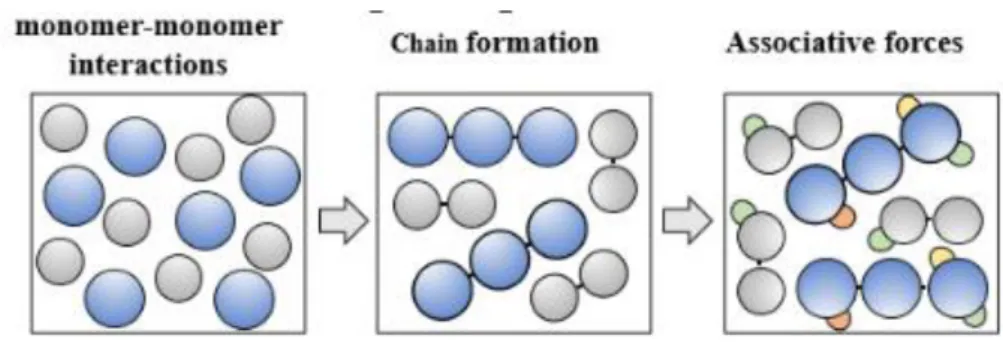
As it can be seen in the Figure 2.1, soft-SAFT represents molecules as a number of equally-sized spherical segments covalently bonded to each other forming chains that may or may not associate at specific sites (i.e. associating species present as association sites for hydrogen bonding).

Figure 2.1Schematic representation of the physical foundation of SAFT-type equations.

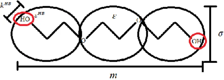
To define the LJ reference fluid, three parameters are required. The chain length parameter (m), the diameter of the monomers or groups sphere that give origin to the molecule (σ) and dispersive energy between the spheres (ε/kB). In soft-SAFT, these three parameters can entirely

11 For self-associating molecules, the association term must be enabled; an association scheme for each associating molecule must be defined specifying the number/type of association sites and interactions allowed in the system. For this, two additional parameters are required, namely the association energy (𝜀𝐻𝐵) and volume (𝑘𝐻𝐵) of the association sites.

Figure 2.2

Schematic representation of the soft-SAFT molecular parameters.

The extension to mixtures is made under the van der Waals one-fluid theory using the generalized Lorentz-Berthelot (LB) mixing rules Equation (2.2) and Equation (2.3).

𝜎𝑖𝑗= 𝜂𝑖𝑗∙ (

𝜎𝑖𝑖+ 𝜎𝑗𝑗

2 )

(2.2)

𝜀𝑖𝑗 = 𝜉𝑖𝑗∙ √𝜀𝑖𝑖∙ 𝜀𝑗𝑗 (2.3)

where 𝜂𝑖𝑗 and 𝜉𝑖𝑗 are the size and energy correction binary parameters, fitted to binary

experimental data.

When cross-association between different species is present, cross-association parameters are given by the following combining rules:

𝜀_𝑖𝑗𝐻𝐵= √𝜀_𝑖𝑖𝐻𝐵_{∙ 𝜀} 𝑗𝑗𝐻𝐵 (2.4) 𝑘_𝑖𝑗𝐻𝐵= ( √𝑘_𝑖𝑖𝐻𝐵 3 + √𝑘3 _𝑗𝑗𝐻𝐵 2 ) 3 _(2.5)

12

One of the advantages of using SAFT-type equations is that the enhanced physical meaning of the model parameters allows to establish correlations of the non-associating molecular parameters as a function of the molecular weight for a given homologous series of compounds enabling the prediction of thermodynamic properties for compounds for which no experimental data is available. This can be done by modelling a few but representative number of members of a compounds’ family and then transfer the molecular parameters to other members of the family not included in the model’s parameterization or for which no experimental data is available. This feature is considered one of the greatest advantages of SAFT-type EoSs, as illustrated by Navarro et al.[37] _{in a careful analysis of soft-SAFT parameters and their possible}

transferability. On the other hand, association parameters can remain constant when the interactions involved are similar. This meaning that the association parameters typically remain constant after the first or first two members of a series of compounds and might be transferable across different species if the same functional group is involved.

An accurate description of transport properties such as dynamic viscosity is vital for the design of several equipment used in industry due to the impact it has on the heat and mass transfer phenomena, fluid dynamics, pressure drops, etc. Different approaches have been proposed to model viscosities, ranging from empirical to highly theoretical methods. Correlations and other empirical methods are computational efficient and provide accurate results, but lack extrapolation ability and therefore, can’t be applied outside the range of experimental data. On the other hand, most theoretical methods, although accurate when describing gas viscosities, fail when used to reproduce the viscosity of dense fluids.

One of the most popular approaches to model the viscosity of dense fluids is the free-volume theory (FVT) proposed by Allal et al.[82],[83]_{. The FVT theory is based in the concept of free}

volume and diffusion models[82]–[85]_.

FVT calculates the viscosity as a sum of two terms: the diluted gas term (η0) and the dense

liquid term (∆𝜂). The diluted-gas term describes the viscosity of a fluid in the very low-density region and is based on the kinetic theory of Chapman-Enskog. This term is neglected in this work given its dependency on critical properties (not available for [Ch]Cl) and the density region of interest for this work that makes of this diluted-gas term negligible if compared to the dense term.

13 The dense term comes from the idea that viscosity is dependent on the empty space between molecules (free-volume) through an exponential relation[86] _{as depicted in Equation}

(2.6). ∆𝜂 = 𝐿𝑣∙ (0.1 ∙ 𝑝 + 10−4∙ 𝛼 ∙ 𝜌2∙ 𝑀𝑤) ∙ √ 10−3_{∙ 𝑀} 𝑊 3 ∙ 𝑅 ∙ 𝑇 ∙ 𝑒𝑥𝑝 𝐵∙(10−3∙𝑝+𝛼∙𝜌_{𝜌∙𝑅∙𝑇}2∙𝑀𝑤) 3 2 (2.6)

The final equation of the dense term includes three adjustable parameters: Lv which is a

length parameter related to the molecule’s structure and relaxation time, B the free-volume overlap and α, which is related to the energy barrier. These parameters should be fitted to available experimental viscosity data, preferably from the pure fluid[86],[87]_{. The Equation (2.6)}

also includes the pressure (𝑝), the density (𝜌), the molecular weight (𝑀𝑤), the ideal gas constant

(𝑅) and the temperature (𝑇).

As it can be observed, the viscosity calculated by the FVT model requires as an input the values of pressure, temperature and density of the system, with the accuracy of the viscosities obtained being heavily dependent on the accuracy of those values. Hence, it is important to have a reliable thermodynamic model (here soft-SAFT) that can be coupled with FVT in order to provide reliable values for such inputs.

Applying the FVT model to mixtures requires the use of mixing rules to obtain the correspondent mixture parameters. Different mixing rules have been proposed in the literature such as those of Polishuk and Yitzhak[88] _{, Baylaucq et al.}[89] _{or a simple linear mixing rule, the}

latter being used in this work Equations (2.7) to (2.9).

𝛼𝑚𝑖𝑥𝑡= ∑ 𝛼𝑖∙ 𝑥𝑖 (2.7)

𝐵𝑚𝑖𝑥𝑡= ∑ 𝐵𝑖∙ 𝑥𝑖 (2.8)

14

where 𝑥𝑖 is the molar fraction of the compound i. It is worth highlighting that no binary

parameters are fitted in the viscosity treatment of mixtures, the model was used in a predictive manner.

2.2 High Pressure Density

Vibrating tube densimeter

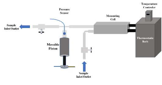
The oscillating U-tube (a tube in a shape of a “U”) is a technique to determine the density of liquids and gases based on the relation between the frequency of oscillation and the density (mass) of the medium. This measuring principle is based on the Mass-Spring Model. A container in a form of a hollow U-shaped glass tube is filled by the sample. This container performs an oscillation which eigenfrequency is influenced by the sample’s mass. The tube is electronically excited into undamped oscillation where the two branches of the U-tube are used as springs. The direction of the oscillation is normal to the level of the branches and only the part of the sample influences the eigenfrequency of the pendulum. The sample mass that participates in the oscillation is always the same since the volume involved in the oscillation is limited by the stationary oscillation knots at the bearing points of the oscillator. In the case of the sample’s volume overfill the oscillator beyond the bearing point, that is irrelevant for the measurement, so the oscillator is capable of measure the density of sample media that flow through the tube. In this work a DMA-HPM, coupled with a MPDS 5-unit, high pressure densimeter from Anton Paar was used to determine the density of the studied compounds in the 283.15 to 373.15 K temperature and 0.1 MPa to 95 MPa pressure ranges. The densimeter has an accuracy of 0.0001 g.cm-3_{, repeatability of 1∙10}-5 _g.cm-3 _{and a resolution of 1∙10}-5 _g.cm-3_{. The temperature of the}

measure cell was controlled with a thermo-regulated fluid (water) from Julabo, model MC, with an uncertainty of 0.01 K and stability of 0.1 K. The pressure was manipulated with a movable piston pressure generator and measured using a Kulite HEM 375 piezoresistive silicon pressure transducer, with accuracy better than 0.2% and uncertainty of 0.03 MPa. To reduce dead volumes the transducer was fixed directly in the ¼ inches stainless steel line and placed between the DMA-HPM measuring cell and the movable piston to avoid dead volumes, as depicted in

Figure 2.3.

The densimeter was calibrated with ultra-pure water (double-distilled, passed through a reverse osmosis system, and further treated with a Milli-Q plus 185 water purification apparatus. It had a resistivity of 18.2 MΩ cm and a total organic carbon smaller than 5 mg∙L-1 _{being free of}

15 particles greater than 0.22 mm), toluene (acquired from Sigma Aldrich, with a mass fraction purity higher than 99.8%) and dichloromethane (acquired from AnalaR NORMAPUR, with a mass fraction purity higher than 99.9%) in the (283 to 363) K, (0.1 to 100) MPa and (0.810 to 1.377) g.cm-3 _{temperature, pressure and density ranges, respectively.}

Figure 2.3Schematic representation of the apparatus of the DMA-HPM measuring cell with the movable piston.

The polynomial suggested by the manufacturer, Equation (2.10), was adopted to calculate the density of the sample within the 0.1-100 MPa pressure, 283.15 – 363.15 K temperature and 0.810 – 1.377 g∙cm-3 _{densityranges. The standard uncertainty on the density was found to be}

5∙10-4 _g·cm−3[90]_.

𝜌 = 𝐴1+ 𝐴2∙ 𝑇 + 𝐴3∙ 𝑝 + 𝐴4∙ 𝑇2+ 𝐴5∙ 𝑝2+ (𝐴6+ 𝐴7∙ 𝑇 + 𝐴8∙ 𝑝 + 𝐴9∙

𝑇2_{+ 𝐴}

10∙ 𝑝2) ∙ 𝑝𝑒𝑟𝑖𝑜𝑑2+ 𝐴11∙ 𝑝𝑒𝑟𝑖𝑜𝑑4

(2.10)

where 𝐴𝑖 is the polynomial coefficients, 𝑇 is the temperature, 𝑝 is the pressure and 𝑝𝑒𝑟𝑖𝑜𝑑 is the

period of oscillation of the hollow tube.

The viscosity of the compounds can influence the density determination due to damping effects inside the vibrating tube, for this reason, the manufacture provided the Equation (2.11) to correct the density. However this correction was not needed since it was verified that the value of the correction was lower than the measurement uncertainty (4.84∙10-4 _g∙cm-3_).

16

With the equipment under vacuum, the sample is injected and the temperature allowed to reach the set point. With the temperature equilibrated the pressures is changed and the the density, at a given temperature and pressure, is determined from the period of oscillation. This procedure is repeated for each intended temperature.

To clean the equipment a peristaltic pump is used to circulate, inside the equipment and through the gas/liquid line, acetone. After the solvent cleaning procedure, the solvent is initially removed by displacement using compressed air and then by applying vacuum (1 Pa) to the system.

2.3 High Pressure Viscosity

Falling Body Viscometer

A body that fall in vacuum conditions, only suffers the force of gravity. No matter the mass of the body, the acceleration that the object is subducted is always the same. However, when an object falls inside a tube filled with a substance this substance imposes an extra resistance to the falling body: the friction resistance. These two forces, gravitational and friction will be balanced at some point of the fall, and when this point is reached, the body is in a called terminal or constant velocity. This principle has been used to measure the viscosity of a substance in the falling body viscometers. In this type of equipment, the body used can be a sphere, a needle or a cylinder (body used in this study).

The operating principle of the equipment used consists on measuring of time that a cylindrical body takes to fall inside a 450 mm length tube with a diameter of 6.52 mm, at a fixed temperature and pressure. The body falls in a way that allows the fluid to ascend through a space between the cylindrical object and the wall of the tube. It is also important that the cylindrical body descends transverse its axis, otherwise the body will suffer more resistance than the expected, and the path described will be larger, leading to larger times and wrong viscosity values. The high pressure viscosity apparatus used was developed by professor Segovia’s group

[91]–[93] _{and shown to be able to determine the viscosity of a large number of fluids within the}

293.15 to 393.15 K temperature, 0.1 to 150 MPa pressure and 0.27 to 1110 mPa∙s viscosity ranges. The equipment was calibrated with toluene, dodecane and 1-butanol and verified, between measurements, by measuring the viscosity, at 298 K, of dioctyl sebacate and squalene.

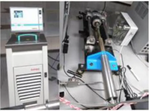
17 The system that measure and control the temperature of the equipment is composed by an Agilent U2352A thermometer, four Pt100 probes to monitor the temperature, with an uncertainty of 0.05 K, and a thermostatic bath from Julabo F25-HE able to control the temperature within 235.15 to 473.15 K with an expanded uncertainty associated to resolution, uniformity and stability of 0.05 K.

Figure 2.4Julabo F25-HE thermostatic bath (left) and Automated pressure generator (right).

To measure the pressure a Druck DPI 104 digital manometer, with a range of (0 to 140) MPa, a resolution of 0.01 MPa, a stability of 0.05 MPa and expand uncertainty associated to the calibration of 0.05 MPa, was used. The setup to control the equipment pressure was made by an automatic triggered cylinder of variable volume from HiP, model 50-6-15 with packing of Teflón B-1066 and 20 cm3 _{controlled by a stepper motor. The results were recorded from a data Agilent}

U2352A data acquisition, an Agilent 34970A thermometer and an Agilent 33220A wave generator.

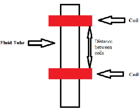
To measure the time that the sinker body takes to travel a defined length, a set of coils placed outside of the measuring cell (separated from each other by 50 mm) were used, as described in Figure 2.5. A wave generator feeds the coils with a sinusoidal signal of 2 Vpp (volts per pulse) and 450 Hz. When the body passes through a coil an excitation in the signal is produced allowing the operator to identify the passage of the magnetic cylindrical body at that point. By identifying the passage of the magnetic cylindrical body in two distinct positions of the cell allows one to determine the cylindrical body travel time through the sample and thus, determine its viscosity using the Equation (2.12).

Initially the apparatus were coupled with four coils. The use of four coils allows to ensure that the body is at terminal speed within the measurement zone however, the presence of four coils produced interferences on the electrical signal imposing thus noise to the measurements.

18

For this reason, it was opted to disconnect the two middle coils during the property determination. Nonetheless, the system’s terminal speed was evaluated, using the four coils, prior to the final viscosity measurements.

Figure 2.5Scheme representing the coils around the measuring tube.

The measuring procedure consists in letting the thermostatic bath reach the desired temperature, set the pressure of the system, rotate the setup to place the falling body at the top of the setup and measure the time that the falling body takes to travel the defined path. The rotation of the setup is made by an automatized rotor.

On the initial runs the apparatus was positioned vertically to the ground, allowing a free fall for the falling body but, analyzing the results it was found that the cylindrical sinker descent was not smooth but colliding against the cell walls. To overcome this problem the apparatus measuring cell was tilted in 0.85 degrees aiming at achieving accurate results. The new angle of operation was nonetheless, taken into account in equipment calibration and then on the property determination.

The viscosity determination was done using Equation (2.12). 𝜂(𝑝, 𝑇) = 𝑡 ∙ (1 −_𝜌𝜌 𝑠) 𝐴 ∙ (1 + 2 ∙ 𝛼𝑣𝑡∙ (𝑇 − 𝑇𝑟𝑒𝑓)) ∙ (1 − 2 ∙ 𝛽𝑣𝑡∙ (𝑝 − 𝑝𝑟𝑒𝑓) 3 ) (2.12)

19 The term time (𝑡) is the time that the sinker body need to cross two consecutive coils, 𝜌 is the density of the fluid at that pressure and temperature, 𝜌𝑠 is the density of the metallic body.∙

𝛼𝑣𝑡 and 𝛽𝑣𝑡 are the coefficient of the thermal expansion and compressibility of the viscometer

tube at the reference conditions of pressure 𝑝𝑟𝑒𝑓 (0.1 MPa) and temperature 𝑇𝑟𝑒𝑓 (298.15 K).

The value of 𝛼𝑣𝑡 and 𝛽𝑣𝑡 are 12.8 ∙ 10−6 𝐾−1 and 4.8 ∙ 10−6 𝑀𝑃𝑎−1, respectively[93]. 𝐴 is the

calibration constant, that is determine by using a well viscosity characterized substance. In the calibration the fluid tube as lightly inclined too so the calibration parameter already is affected by this modification on the equipment.

The equipment requires a sample volume of 120 mL that is introduced into the apparatus using a separation funnel connected to the inlet valve located in the top part of the measuring cell and that do not allow the entrance of the cell. Once the cell and pressure line are filled, starting from a vacuum condition, the valve is closed and the temperature and pressure allowed to reach the desired values; once the desired temperature and pressure was reached the measuring procedure was initiated.

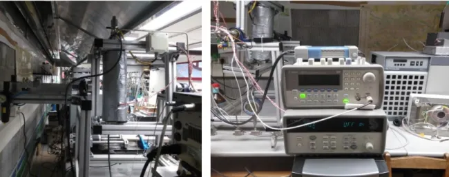
Figure 2.6 Measuring cell (left) and monitoring setup (rigth) composed by an Agilent 34970A thermometer, Agilent 33220A wave generator and Agilent U2352A data acquisition.

To clean the equipment, a solvent miscible with the measuring fluid is allowed to path through the viscometer. Then, the solvent is removed by vacuum and the setup further cleaned with acetone to assure that the interior of the equipment is clean and dried after applying vacuum with a TRIVAC D8B vacuum pump coupled with a cold trap TK 4-8. The setup was considered clean when the pressure reaches 5 ∙ 10−2mbar.

20

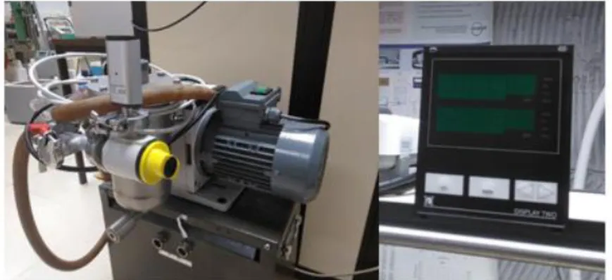
Figure 2.7From the left to the right, the TRIVAC D8B vacuum pump with the cold trap TK 4-8 and the Pirani vacuum measurer.

Vibrating Wire Viscometer

By detailed analysis of a fluid flow around a wire, as well as the mechanical motion of the wire, it can be obtained the viscosity of the fluid. The principle used in this equipment is based in a wire that vibrates in two different oscillation modes, a forced mode and a transient mode. In the forced mode the wire vibrates in a frequency that covers its first harmonic, and the viscosity can be obtained by the width of the resonance signal. In the transient mode the wire vibrated for a short time and then stop, and the viscosity can be calculated from the decay time. The technique consists of a tungsten cylindrical wire surrounded by a fluid, of unknown viscosity, in which a constant sinusoidal current is supplied. This current together with the constant magnetic field, make the wire produce a vibration which generate a electromotive force (EMC) that is measured with a lock-in amplifier in two stages. The value of the EMC is the sum of the terms 𝑉1

and 𝑉2, whose determination can be made by Equation 2.13 and 2.14, respectively. 𝑉1 is the

voltage of the impedance on the wire and 𝑉2 is the wire movement and is proportional to the

speed of the wire.

𝑉1= 𝑎 + 𝑖 ∙ 𝑏 + 𝑖 ∙ 𝑐 ∙ 𝑓 (2.13)

𝑉2=

𝑖 ∙ Λ ∙ 𝑓

𝑓0− (1 + 𝛽) ∙ 𝑓2+ (𝛽′+ 2 ∙ ∆0) ∙ 𝑓2∙ 𝑖

(2.14)

In the Equation (2.13), 𝑓 is the frequency, 𝑖 is the imaginary number, a, b and c are adjustable parameters determined by regression that accounts for the electrical impedance of

21 the wire and the offset used in the lock-in amplifier. In Equation (2.14), Λ is the amplitude, 𝑓 is the driven frequency, 𝑓0 is the resonance frequency in vacuum, ∆0 is the logarithmic decrement

of the wire in vacuum, 𝛽 ( 𝛽 = 𝑘 ∙_𝜌𝜌

𝑠 ) is the additional mass of the fluid, 𝛽

′ _(𝛽′ _{= 𝑘}′_∙ 𝜌

𝜌𝑠) is the damping due to the fluid viscosity, 𝜌𝑠 is the density of the wire, 𝑘 and 𝑘′ are functions of Ω =

(2 ∙ 𝜋 ∙ 𝑓 ∙ 𝜌 ∙ 𝑅2_{)/𝜂, and here 𝜌 is the density and 𝑅 is the radius of the wire. Considering that}

𝑓02= (1 + 𝛽) ∙ 𝑓𝑟2, and rearranging the Equation (2.14), then Equation (2.15) is obtained.

𝜂 =𝜋∙𝑓𝑟∙𝑅2∙𝜌 6 ∙ ( 𝑓_𝑏 𝑓_𝑟) 2 ∙ (1 +𝜌𝑠 𝜌) 2 (2.15)

where 𝑓𝑟 is the resonance frequency and 𝑓𝑏 is the half-width of the resonance curve.

The temperature control of the equipment is made by a thermostatic bath Hart Scientific model 6020 that has a stability of 0.01 K and can work in a range of temperatures between 20 ºC and 100 ºC. The measurement of the temperature of the equipment is made by a ASL F-100 and two platinum Pt100 probes inside the bath and calibrated by comparison with calibrated PRT25Ω probes. The uncertainly of the probes was determined to be 0.02 K in the 233.15 K to 503.15 K temperature range.

As in the case of the falling body viscometer, the equipment is pressurized up to 140 MPa with a cylinder of variable volume operated manually. The pressure generator cylinder, a Hip 68-5.75-10, can operate between 0.1 MPa and 140 MPa. The pressure is measured with a digital manometer General Electric DRUCK DPI 104 with a resolution of 0.01 MPa. This manometer was calibrated in Termocal Laboratory with an uncertainty of 0.02%.

Figure 2.8 Vibrating wire viscometer with a manual pressure generator and the separation funnel from which the sample is introduced.

Separation

funnel

Movable

Piston

22

The setup was calibrated with reference substances, more specifically, dioctyl sebacate, squalene and dodecane showing a viscosity combined standard uncertainty of 1%.

To clean the equipment, water was used as solvent. The solvent is introduced through the separation funnel, in a similar way as the sample, and allowed to fill the setup. Then the variable volume cylinder (piston) is moved back and forward to ensure a complete and efficient cleaning procedure. These steps are performed several times until all the solvent is removed by compressed air displacement and vacuum. To ensure a complete clean setup a final cleaning procedure using acetone is performed.

SVM 3000 Anton Paar rotational Stanbinger viscometer-densimeter

The viscometer is based in a hollow tube filled with the sample and a magnetic rotor. The low density of the rotor (lighter than the sample) allows it to be centered in the liquid by buoyancy forces and the rotor is always in the same axial position due to an embedded magnet in the rotor that interact with a soft iron ring located outside the tube. The buoyancy forces create a gap between the rotor and the inside hall of the tube which force the rotor to rotate by shear stresses in the liquid. The rotation of the rotor generates a rotational magnetic field transmits a speed signal and induces eddy currents in the copper jacket that covers in tube. The speed of the rotor is influencing the eddy currents and exerts a retarding torque of the rotor. The equilibrium between the torque caused by the eddy currents and the sample cause a constant rotation of the rotor and then the viscosity of the sample can be determined. The viscometer has a temperature uncertainty of 0.02 K between 288.15 K and 378.15 K, the relative uncertainty of the measured dynamic viscosity is 1% and the uncertainty of the density is 0.0005 g∙cm-3_.

The equipment is cleaned passing a solvent miscible with the sample, using a peristaltic pump, then the solvent is displaced and the setup dried using dry air.

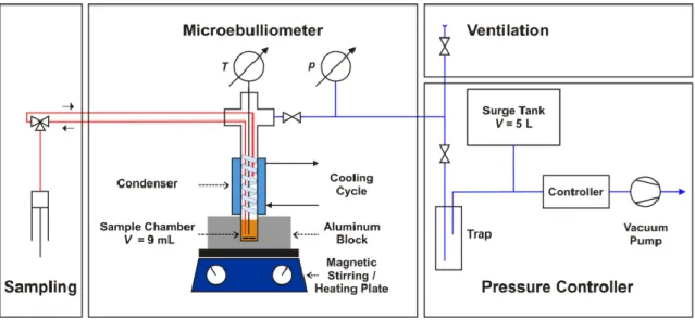
2.4 Isobaric ebulliometer

An isobaric ebulliometer able to operate at pressures ranging from 0.05 up to 0.1 MPa, was designed, assembled and tested in our laboratory. The ebulliometer, schematically presented in Fig. 2.7, is composed by three sections: a glass sample chamber container, with a total volume of8 ml, that is placed inside of an aluminum block placed on top of a heating/stirring plate; a

23 glass condenser, surrounding the top section of the apparatus sample chamber, where the temperature is kept constant by means of a thermostatic bath; a liquid sampling/injection, a temperature prove and pressure line connections, done by means of vacuum tide Teflon sealed ports. Inside the ebulliometer top section a removable glass spiral increases the surface area of the reflux/condenser and the condenser, placed immediately above the sample chamber and connected to a thermostatic bath to assure a better condensation of the vapor phase generated. A Teflon-coated magnetic stirring bar, placed in the sample chamber, allows to maintain the temperature and the concentration of the sample homogeneous during the experimental procedure. The sampling/injection procedure is made by a silicone tube that passes thought one of the Teflon sealed ports and connected to the sample chamber. The temperature of the liquid phase, inside the ebulliometer is measured by means of a type K thermocouple previously calibrated against a platinum resistance thermometer, SPRT100 (Fluke-Hart Scientific 1529 Chub-E4), traceable to the National Institute of Standards and Technology (NIST) with an uncertainty of less than 2∙10-2 _{K. The pressure is maintained constant through a vacuum line with 5∙10}-3 _m3

internal volume and connected to a Büchi V-700 vacuum pump and V-850 pressure monitoring and controller unit. The measuring of the pressure is made by a Baratron type capacitance Manometer, MKS model 728A with an accuracy of 0.5%. In the aluminum block there is a metallic sealed Pt100 class A temperature probe that allow the determination of the temperature difference between the sample and the block, this information helps to know if there a vapor-liquid equilibrium in the system or not.

A mixture of unknown composition is placed inside the ebulliometer and allowed to reach equilibrium, with constant and smooth boiling. Once the equilibrium is reached, the boiling temperature is measured, the liquid phase sample and the mixture composition determined through an Anton Paar Abbemat 500 Refractometer, with an uncertainty of 2∙10-5 _{nD, using a}

calibration curve previously established. The compositions have an uncertainty of 2∙10-5 _g.

To clean the setup, the ebulliometer is removed from the apparatus and disconnected from the circulator thermostatic bath. Then the ebulliometer’ silicon tube and the glass spiral are removed, washed and dried.

24

Figure 2.9 Schematic representation of the isochoric ebulliometer, figure taken from

25

26

3.1 Eutetic Systems

Choline Chloride ([Ch]Cl), Ethylene Glycol (EG), Glycerol (Gly) and Urea were acquired from Acros Organics, Sigma Aldrich and Analar+Sigma with mass fraction purity of 98%, 99.5%, 99% and 99.5%, respectively. The compounds chemical structure, purity, supplier, and corresponding designations are presented in Table 3.1. It is well established that even small amounts of water and other impurities have a great impact in the compound’s properties, especially on transport properties like viscosity. Therefore, with the exception of urea, that was used as received from the supplier, all the other substances were submitted to a purification methodology. Individual samples of [Ch]Cl were dried at moderate temperatures (323 K), vacuum (1 Pa) and under continuous stirring for a period never smaller than 48 hours.

Ethylene glycol and glycerol vapor pressures (18.28 and 0.04 Pa at 303 K, respectively) do not allow to adopt the purification procedure, with a vacuum of 1 Pa, adopted for the choline chloride and thus, aiming at lowering the water content the compounds were stored in a glass flask in contact with 3 Å zeolites for a minimum of 12h. The final water content, after the drying step and immediately before the mixtures preparation, was determined with a Metrohm 831 Karl Fischer coulometer (using the Hydranal−Coulomat AG from Riedel-de Haën as analyte). The average water content was found to be lower than 100 ppm.

3.2 Samples Preparation

Preparation of [Ch]Cl + Urea

While urea was used directly has received from the supplier the choline chloride was purified using the abovementioned procedure. In order to avoid water absorption, from atmosphere, choline chloride was weighted using an analytical balance model ALS 220-4N from Kern with an accuracy of 0.002 g inside a dry-argon glove-box, which provides an atmosphere low in oxygen and moisture with less than 1 ppm and 2 ppm respectively. Urea is a low hygroscopic compound, so, it was weighted using a Sartorius analytical balance (with an uncertainty of 0.001 g) outside the glove-box. The mixture with a composition close to the eutectic point, 1 mol of [Ch]Cl to 2 mol of urea, was prepared at room temperature in a closed

27 Erlenmeyer containing a magnetic bar; At room temperature both compounds are solid and thus, the mixture was gradually heated in a hot plate with constant stirring, until complete homogenization, and under vacuum (1 Pa). The compounds’ weight and choline chloride mole fraction of the mixture are reported in Table 1.2 and Table 1.3.

Table 3.1. Chemical structure, compound description, CAS number, molecular weight, mass

fraction purity, and supplier of the compounds studied in this work.

Compound CAS Mw Purity

(%) Supplier Chemical Structure

Choline Chloride 67-48-1 139.6 2 98% Acros Organics Ethylene

Glycol 107-21-1 62.07 99.5% Sigma Aldrich

Glycerol 56-81-5 92.09 99% Acros

Organics

Urea 57-13-9 60.06 99.5% Analar+Sigma

Preparation of [Ch]Cl + EG and [Ch]Cl + Gly

The mixtures were prepared analytically with a composition close to the eutectic point, 1 mol of salt to 2 mol of HBD. The choline chloride was weighted using an analytical balance model ALS 220-4N from Kern with an accuracy of 0.002 g inside the dry-argon glove-box and the EG or the Gly were weighted using a Mottler Toledo balance with an uncertainty of 0.0001 g. The mixture was allowed to homogenize under continuous stirring. The compounds’ weight and choline chloride mole fraction of the mixture are reported in Table 1.2 and Table 1.3.