Control and management mechanisms in 5G networks: operator networks

(1)

Universidade de Aveiro Departamento de Eletrónica,Telecomunicações e Informática 2019

Diogo Daniel

Soares Ferreira

Mecanismos para controlo e gestão de redes 5G:

Redes de Operador

Control and management mechanisms in 5G

networks: Operator networks

(2)

(3)

✏❲❡ ❝❛♥ ♦♥❧② s❡❡ ❛ s❤♦rt ❞✐st❛♥❝❡ ❛❤❡❛❞✱ ❜✉t ✇❡ ❝❛♥ s❡❡ ♣❧❡♥t② t❤❡r❡ t❤❛t ♥❡❡❞s t♦ ❜❡ ❞♦♥❡✳✑

✖ ❆❧❛♥ ❚✉r✐♥❣ Universidade de Aveiro Departamento de Eletrónica,Telecomunicações e Informática 2019

Diogo Daniel

Soares Ferreira

Mecanismos para controlo e gestão de redes 5G:

Redes de Operador

Control and management mechanisms in 5G

networks: Operator networks

(4)

(5)

Universidade de Aveiro Departamento de Eletrónica,Telecomunicações e Informática 2019

Diogo Daniel

Soares Ferreira

Mecanismos para controlo e gestão de redes 5G:

Redes de Operador

Control and management mechanisms in 5G

networks: Operator networks

Dissertação apresentada à Universidade de Aveiro para cumprimento dos requisitos necessários à obtenção do grau de Mestre em Engenharia de Computadores e Telemática, realizada sob a orientação científica da Profes-sora Doutora Susana Sargento, ProfesProfes-sora Catedrática do Departamento de Eletrónica, Telecomunicações e Informática da Universidade de Aveiro, e do Doutor Carlos Senna, Investigador do Instituto de Telecomunicações.

(6)

(7)

o júri / the jury

presidente / president Professor Doutor Amaro Fernandes de Sousa

professor auxiliar do Departamento de Eletrónica, Telecomunicações e Informática da Universi-dade de Aveiro (por delegação do Vice-Reitor da UniversiUniversi-dade de Aveiro)

vogais / examiners committee Professor Doutor Rui Lopes Campos

professor auxiliar convidado da Faculdade de Engenharia da Universidade do Porto (arguente)

Professora Doutora Susana Sargento

professora catedrática do Departamento de Eletrónica, Telecomunicações e Informática da Uni-versidade de Aveiro (orientadora)

(8)

(9)

agradecimentos /

acknowledgements

Em primeiro lugar, agradeço à minha família, em especial aos meus pais e aos meus irmãos, não só pelo apoio total que me deram ao longo de toda a minha vida, mas também pela paciência que tiveram durante estes 5 anos de trabalho e estudo intenso.

Agradeço à Professora Doutora Susana Sargento e a todo o grupo de inves-tigação Network Architectures and Protocols (NAP) o excelente acolhimento, apoio incondicional e todos os ensinamentos obtidos durante estes dois anos e meio de trabalho conjunto, onde sempre me foi dada a liberdade para desen-volver projetos de acordo com a minha vontade pessoal. Um agradecimento especial ao Doutor André Reis e ao Professor Doutor Paulo Salvador pelas discussões sobre Machine Learning, e também ao Doutor Carlos Senna pela ajuda na escrita desta dissertação.

Um grande agradecimento a todos os meus amigos que conheci durante este percurso, pelos momentos de descontração, pelos almoços, mas também pelas discussões interessantes sobre os mais variados temas, incluindo o trabalho apresentado nesta dissertação. Obrigado também a todos os pro-fessores que contribuíram para o meu crescimento académico.

Muito obrigado a todos os que direta e indiretamente contibuíram para a con-clusão do meu mestrado.

Finalmente, um grande obrigado a Ele, sem o qual nada disto seria possível. Agradeço à Fundação Portuguesa para a Ciência e Tecnologia pelo suporte fi-nanceiro com fundos nacionais e europeus através Fundo Europeu de Desen-volvimento Regional (FEDER), no âmbito do Programa Operacional Regional de Lisboa (POR LISBOA 2020) e do Programa Operacional de Competitivi-dade e Internacionalização (COMPETE 2020) do Portugal 2020 (POCI-01-0247-FEDER-024539).

(10)

(11)

Palavras Chave

Previsão de séries temporais, 5G, Monitorização de rede, Aprendizagem Au-tomática, Arquitetura de Previsão, Políticas de rede, Slicing de rede.

Resumo

Em redes 5G, séries temporais serão omnipresentes para a monitorização

de métricas de rede. Com o aumento do número de dispositivos da Internet das Coisas (IoT) nos próximos anos, é esperado que o número de fluxos de séries temporais em tempo real cresça a um ritmo elevado. Para monitorizar esses fluxos, testar e correlacionar diferentes algoritmos e métricas simul-taneamente e de maneira integrada, a previsão de séries temporais está a tornar-se essencial para a gestão preventiva bem sucedida da rede.

O objetivo desta dissertação é desenhar, implementar e testar um sistema de previsão numa rede de comunicações, que permite integrar várias redes diferentes, como por exemplo uma rede veicular e uma rede 4G de opera-dor, para melhorar a fiabilidade e a qualidade de serviço (QoS). Para isso, a dissertação tem três objetivos principais: (1) a análise de diferentes data-sets de rede e subsequente implementação de diferentes abordagens para previsão de métricas de rede, para testar diferentes técnicas; (2) o desenho e implementação de uma arquitetura distribuída de previsão de séries tem-porais em tempo real, para permitir ao operador de rede efetuar previsões sobre as métricas de rede; e finalmente, (3) o uso de modelos de previsão criados anteriormente e sua aplicação para melhorar o desempenho da rede utilizando políticas de gestão de recursos.

Os testes efetuados com dois datasets diferentes, endereçando os casos de uso de gestão de congestionamento e divisão de recursos numa rede com recursos limitados, mostram que o desempenho da rede pode ser melhorado com gestão preventiva da rede efetuada por um sistema em tempo real capaz de prever métricas de rede e atuar em conformidade na rede.

Também é efetuado um estudo sobre que métricas de rede podem causar reduzida acessibilidade em redes 4G, para o operador de rede atuar mais eficazmente e proativamente para evitar tais acontecimentos.

(12)

(13)

Keywords

Time-series prediction, Forecasting, 5G, Network Monitoring, Machine Learn-ing, Prediction Architecture, Network Policies, Network Slicing.

Abstract

In 5G networks, time-series data will be omnipresent for the monitoring of net-work metrics. With the increase in the number of Internet of Things (IoT) de-vices in the next years, it is expected that the number of real-time time-series data streams increases at a fast pace. To be able to monitor those streams, test and correlate different algorithms and metrics simultaneously and in a seamless way, time-series forecasting is becoming essential for the pro-active successful management of the network.

The objective of this dissertation is to design, implement and test a prediction system in a communication network, that allows integrating various networks, such as a vehicular network and a 4G operator network, to improve the net-work reliability and Quality-of-Service (QoS). To do that, the dissertation has three main goals: (1) the analysis of different network datasets and imple-mentation of different approaches to forecast network metrics, to test differ-ent techniques; (2) the design and implemdiffer-entation of a real-time distributed time-series forecasting architecture, to enable the network operator to make predictions about the network metrics; and lastly, (3) to use the forecasting models made previously and apply them to improve the network performance using resource management policies.

The tests done with two different datasets, addressing the use cases of con-gestion management and resource splitting in a network with a limited number of resources, show that the network performance can be improved with pro-active management made by a real-time system able to predict the network metrics and act on the network accordingly.

It is also done a study about what network metrics can cause reduced ac-cessibility in 4G networks, for the network operator to act more efficiently and pro-actively to avoid such events.

(14)

(15)

List of Figures

1.1 Ericsson projection for the number of cellular IoT connections in the next years. . . 2

2.1 Illustration of the Fault, Configuration, Accounting, Performance and Security (FCAPS) model. . 7 2.2 Illustration of the Business Process Framework (eTOM) process model. . . 8 2.3 Illustration of the Simple Network Management Protocol (SNMP) entities. . . 10 2.4 Some 5G use cases grouped by the type of interaction and the range of performance requirements [20]. 12 2.5 Software-Defined Network architecture [28]. . . 13 2.6 Network Functions Virtualization (NFV) reference architectural framework [32]. . . 14 2.7 5G network slices example. Above a multi-vendor and multi-access physical infrastructure, there

are logical slices independently managed, each one of them addressing a specific use case [33]. . . . 15 2.8 Reference architecture of Framework for self-organized network management in virtualized and

software-defined networks (SELFNET) framework [36]. . . 17 2.9 Selfnet control loop [36]. . . 18 2.10 Control, Orchestration, Management, Policy and Analytics (COMPA) Autonomic control loop [37]. 18 2.11 COMPA Architecture & Responsability domains [37]. . . 19 2.12 Open Network Automation Platform (ONAP) Casablanca architecture5

, November 2018. . . 20 2.13 5G Novel Radio Multiservice adaptative network Architecture (5G NORMA) functional architecture

[41]. . . 21 2.14 Architecture of the CogNet Project [42]. . . 22 2.15 5G cognitive management architecture [4]. . . 23 2.16 Example of an architecture of an Artificial Neural Network (ANN) with two hidden layers with

four neurons each, with 3 neurons in the input layer and only one neuron in the output layer. . . . 25 2.17 General architecture of a recurrent neural network. . . 26 2.18 Internal architecture of an Long Short-Term Memory Neural Network (LSTM) cell3

[Adapted]. . . 27 2.19 Example of a 1-D convolutional layer [51]. . . 27

3.1 Approach proposed by Madan and Mangipudi [68], where the network traffic is divided in two components before the predictions are applied for each component, and then are added again to obtain the final forecasts. . . 32

(20)

3.2 Combination of convolutional layers and LSTM layers in the proposed architecture in [85]. . . 36 3.3 Robust statistical Traffic Classification (RTC) framework [75]. . . 38

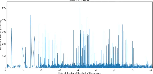
4.1 Sessions’ duration over time, in minutes. The three markers show the periods where there were no sessions in the vehicular dataset. . . 44 4.2 Sessions’ duration in minutes in the day of 14th

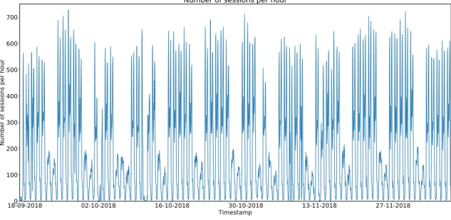
of Octoboer of 2018 in the vehicular network. . . 45 4.3 Number of sessions per hour in the vehicular network. . . 45 4.4 Number of sessions per hour limited to the data used for forecasting, in the vehicular network. . . 46 4.5 Number of sessions per hour of one week in the vehicular network. . . 46 4.6 Number of sessions per hour of a week with a national holiday in the 1st of November (i) in the

vehicular network. . . 47 4.7 Number of sessions per hour over time, with the rolling mean and rolling standard deviation

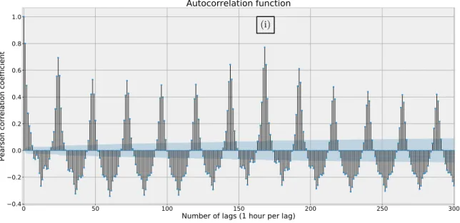
represented, with a rolling window of 24 hours, in the vehicular network. . . 48 4.8 Autocorrelation plot of the time series data in the vehicular network. . . 48 4.9 Seasonal decomposition using moving averages with an additive model and frequency of one week

in the vehicular network. The first plot shows the original data; the second shows the captured trend; the third plot shows the seasonality; the last plot shows the residuals. . . 49 4.10 Number of sessions per hour in consecutive hours in the vehicular network. . . 50 4.11 Time-series data histogram of the vehicular network. . . 50 4.12 Time-series data of the vehicular network with differentiation of one lag, with the rolling mean and

rolling standard deviation represented, with a rolling window of 24 hours. . . 51 4.13 Autocorrelation plot of the time-series of the vehicular network data with differentiation of one lag. 52 4.14 Seasonal decomposition of the vehicular network with a one-lag differentiation using moving averages

with additive model and frequency of one week. The first plot shows the original data; the second shows the captured trend; the third plot shows the seasonality; the last plot shows the residuals. . 52 4.15 Time-series data of the vehicular network with differentiation of 24 lags, with the rolling mean and

rolling standard deviation represented, with a rolling window of 24 hours. . . 53 4.16 Autocorrelation plot of the vehicular network with differentiation of 24 lags. . . 53 4.17 Seasonal decomposition of the vehicular network with a 24-lags differentiation using moving averages

with additive model and frequency of one week. The first plot shows the original data; the second shows the captured trend; the third plot shows the seasonality; the last plot shows the residuals. . 54 4.18 Vehicular network data with differentiation of 168 lags, with the rolling mean and rolling standard

deviation represented, with a rolling window of 24 hours. . . 54 4.19 Autocorrelation plot of the vehicular network data with differentiation of 168 lags. . . 55 4.20 Seasonal decomposition of the vehicular network with a 168-lags differentiation using moving

averages with additive model and frequency of one week. The first plot shows the original data; the second shows the captured trend; the third plot shows the seasonality; the last plot shows the residuals. . . 55 4.21 Vehicular network dataset split in training set, cross-validation set and test set. . . 56 4.22 Forecasts made by the persistence model with K=168 in the cross-validation set of the vehicular

(21)

4.23 Forecasts made by the ARIMA model in the cross-validation set of the vehicular network, with the order parameters (3,168,0), compared with the real values. . . 60 4.24 Average RMSE for classical machine learning algorithms varying the differentiation lag. . . 62 4.25 Average RMSE for classical machine learning algorithms varying the number of lags as input. . . . 62 4.26 Prediction made by the Random Forest model in the cross-validation setof the vehicular network,

with 168-lag differentiation and 12 input lags, compared with the real values. . . 63 4.27 Average Root Mean Squared Error (RMSE) for classical machine learning algorithms varying the

number of lags as input with all the additional features added in the input. . . 64 4.28 Prediction made by the Random Forest model in the cross-validation set of the vehicular network,

compared with the real values, with a RMSE of 36.3 sessions per hour. . . 65 4.29 Training and cross-validation RMSE variation with the number of trained epochs for the model

number 1 with no differentiation and lag number of 12. . . 68 4.30 Training and cross-validation RMSE variation with the number of trained epochs for the model

number 5 with no differentiation and lag number of 24. . . 69 4.31 Training and cross-validation RMSE variation with the number of trained epochs for the model

number 23 with one-lag differentiation and lag number of 12. . . 69 4.32 Forecasts made by the best feed-forward neural network model in the cross-validation set of the

vehicular network, compared with the real values, with a RMSE of 29.99 sessions per hour and a Mean Absolute Percentage Error (MAPE) of 23.26%. . . 70 4.33 Prediction made by the best recurrent neural network model in the cross-validation set of the

vehicular network, compared with the real values, with a RMSE of 31.36 sessions per hour and a MAPE of 31.72%. . . 72 4.34 Training and cross-validation RMSE variation with the number of trained epochs for the model

number 4, with a lag number of 12, with a Global Max Pooling layer and with batch normalization. 74 4.35 Training and cross-validation RMSE variation with the number of trained epochs for the model

number 11, lag number of 24, with a Flatten layer and batch normalization. . . 75 4.36 Training and cross-validation RMSE variation with the number of trained epochs for the model

number 2, with a lag number of 12, with a Global Max Pooling Layer and no batch normalization. 75 4.37 Training and cross-validation RMSE variation with the number of trained epochs for the model

number 2, with a lag number of 12, with a Flatten and no batch normalization. . . 76 4.38 Forecasts made by the best 1-D convolutional neural network model in the cross-validation set of

the vehicular network, compared with the real values, with a RMSE of 38.59 sessions per hour. . . 76 4.39 Prediction made by the Random Forest model in the cross-validation set of the vehicular network,

with the set of features 6, with a RMSE of 38.45 sessions per hour. . . 79 4.40 Forecasts made by the ensemble model with three predictors in the cross-validation set of the

vehicular network, compared with the real values, with a RMSE of 26.22 sessions per hour. . . 81 4.41 Forecasts made by the ensemble model with three predictors in the test set of the vehicular network,

compared with the real values, with a RMSE of 22.11 sessions per hour. . . 82

5.1 Plot with the observations of the test set, showing the thresholds with σ = 0.2, σ = 0.5 and

σ= 0.8. The dots are the observations used to calculate the Root Mean Squared Error above Threshold (RMSET) above each threshold. . . 87

(22)

5.2 Plot with the observations of the test set, showing the thresholds with σ = 0.2, σ = 0.5 and σ = 0.8. The dots are the observations used to calculate the Differentiated Root Mean Squared Error above Threshold (DRMSET) above each threshold. . . 88 5.3 Forecasts made by an ensemble of the three models optimized for the lowest RMSET (σ=0.8) in

the test set compared with the real values. . . 89 5.4 Number of sessions per hour in the Porto public buses from the 12th

of December of 2018, at 08:00:00, to the 11th

of January of 2019, at 13:00:00. . . 92 5.5 Seasonal decomposition using moving averages with additive model and frequency of one week.

The first plot shows the original data; the second plot shows the captured trend; the third plot shows the seasonality; the last plot shows the residuals. . . 93 5.6 Autocorrelation plot of the time series data. . . 93 5.7 Train set with one-lag differentiation applied. . . 94 5.8 Test set with one-lag differentiation applied. . . 94 5.9 Training set with one-lag multiplicative transformation applied. . . 95 5.10 Test set with one-lag multiplicative transformation applied. . . 96 5.11 Value for the RMSE performance metric for the training set and test set along the number of

trained epochs. . . 97 5.12 Forecasts made on the test set compared to the real observations. The model used was the test

number five with one-lag differentiation. . . 97

6.1 Maximum number of connected users per hour. The maximum values on the weekend days are marked with a circle. . . 101 6.2 Maximum number of active users per hour. . . 101 6.3 Maximum number of connected users per hour in a cell. . . 102 6.4 Maximum number of connected users per hour in a cell. . . 102 6.5 Rolling mean and standard deviation of the number of connected users along the month. . . 103 6.6 Autocorrelation plot for the maximum number of connected users. . . 104 6.7 Histogram of the connected users in the network. . . 104 6.8 Seasonal decomposition using moving averages with an additive model and frequency of one week.

The first plot shows the original data; the second plot shows the captured trend; the third plot shows the seasonality; the last plot shows the residuals. . . 105 6.9 Rolling mean and standard deviation of the number of connected users along the month with

one-lag differentiation. . . 106 6.10 Autocorrelation plot for the maximum number of connected users differentiated by one lag. . . 106 6.11 Seasonal decomposition using moving averages with an additive model and frequency of one week.

The first plot shows the original data; the second plot shows the captured trend; the third plot shows the seasonality; the last plot shows the residuals. . . 107 6.12 Rolling mean and standard deviation of the number of connected users along the month with 24-lag

differentiation. . . 107 6.13 Autocorrelation plot for the maximum number of connected users differentiated by 24 lags. . . 108

(23)

6.14 Seasonal decomposition using moving averages with an additive model and frequency of one week. The first plot shows the original data; the second plot shows the captured trend; the third plot shows the seasonality; the last plot shows the residuals. . . 108 6.15 Rolling mean and standard deviation of the number of connected users along the month with

168-lag differentiation. . . 109 6.16 Autocorrelation plot for the maximum number of connected users differenced by 168 lags. . . 109 6.17 Seasonal decomposition using moving averages with an additive model and frequency of one week.

The first plot shows the original data; the second plot shows the captured trend; the third plot shows the seasonality; the last plot shows the residuals. . . 110 6.18 Dataset division in train, cross-validation and test set. . . 111 6.19 Forecasts made by the persistence model with K=1 in the cross-validation set, compared with the

real values. . . 112 6.20 Prediction made by the ARIMA model in the cross-validation set with the order parameters (2,0,4)

compared with the real values. . . 113 6.21 Average RMSE for classical machine learning algorithms varying the differentiation lag. . . 114 6.22 Average RMSE for classical machine learning algorithms varying the number of lags as input. . . . 115 6.23 Forecasts made by the SVR model in the cross-validation set compared with the real values, with a

RMSE of 127.49 sessions per hour. . . 115 6.24 Forecasts made by the best feed-forward neural network model in the cross-validation set compared

with the real values, with a RMSE of 115.54 sessions per hour. . . 118 6.25 Forecasts made by the best recurrent neural network model in the cross-validation set compared

with the real values, with a RMSE of 113.70 connected users per hour. . . 120 6.26 Foreacsts made by the ensemble model with two predictors in the cross-validation set compared

with the real values, with a RMSE of 104.94 maximum connected users per hour. . . 121 6.27 Forecasts made by the ensemble model with two predictors in the test set compared with the real

values, with a RMSE of 152.41 connected users per hour. . . 122

7.1 Sequence diagram indicating the E-UTRAN Radio Access Bearer (E-RAB) setup phase. . . 124 7.2 Number of E-RAB setup failures. . . 124 7.3 F1-score with different algorithms varying the number of Principal Component Analysis (PCA)

components for the task (i) for the aggregated network. . . 129 7.4 F1-score with different algorithms varying the number of PCA components for the task (ii) for the

aggregated network. . . 129 7.5 F1-score with different algorithms varying the number of PCA components for the task (i) for the

individual cells tests. . . 131 7.6 F1-score with different algorithms varying the number of PCA components for the task (ii) for the

individual cells tests. . . 132

8.1 Overall architecture of the prediction architecture. . . 136 8.2 Data visualization with Grafana plugin. . . 140

(24)

9.1 Percentage of lost sessions for both slices, varying according to the maximum number of sessions in the 4G slice, for a maximum of 3000 sessions in the network. . . 144 9.2 Number of sessions in a week of the test set of the 4G slice, with the threshold of 2580 sessions. . 145 9.3 Number of sessions in a week of the test set of the vehicular slice, with the threshold of 420 sessions.145 9.4 Percentage of sessions lost varying the sessions available in the network for different algorithms. . 148 9.5 Percentage of sessions lost varying the sessions available in the network for different algorithms, in

detail. . . 148 9.6 Reactive management of the congestion threshold in the vehicular slice. . . 149 9.7 Reactive management of the congestion threshold in the 4G slice. . . 150 9.8 Reactive management of the congestion threshold in the network. . . 150 9.9 Pro-active management of the congestion threshold in the vehicular slice. . . 151 9.10 Pro-active management of the congestion threshold in the 4G slice. . . 151 9.11 Pro-active management of the congestion threshold in the network. . . 152

(25)

List of Tables

4.1 RMSE and MAPE values of the persistence model with different value of K. . . 58 4.2 RMSE results for the forecast with the Autoregressive integrated moving average (ARIMA) model

for different d values. . . . 59 4.3 RMSE results for the forecast with the ARIMA model for different p values. . . . 59 4.4 RMSE results for the forecast with the ARIMA model for different q values. . . . 59 4.5 Ten best results of the ARIMA approach in the forecasting. . . 60 4.6 The eight different set of combinations for testing additional features. For each set of tests, for

each feature, if the entry is True, the feature was used. Otherwise, the feature was not used. . . . 64 4.7 Average RMSE for the forecasts for different combinations of additional features. . . 64 4.8 Best results for each set of tests using different additional features, with the best algorithm, its

hyper-parameters, RMSE and MAPE. . . 65 4.9 Configurations tested for the feed-forward neural network. . . 66 4.10 Average RMSE for the forecast with the feed-forward neural networks for different number of input

lags. . . 67 4.11 Average RMSE for the forecast with the feed-forward neural networks for varying differentiation lags. 67 4.12 Average RMSE results for each network configuration . . . 67 4.13 Ten best results on the tests using a feed-forward neural network. . . 68 4.14 RMSE result for the different set of tests with additional features, made only to the previous ten

best results. . . 70 4.15 Configurations tested for the recurrent neural network. . . 71 4.16 Ten best results obtained using a recurrent neural network. . . 72 4.17 RMSE for the tests with different combinations of additional features, for the best model for the

recurrent neurl networks. . . 72 4.18 Different network configurations used for testing the 1-D convolutional networks. Each model

described was tested with and without batch normalization and with Flatten and Global Max Pooling. . . 74 4.19 Best RMSE results in the 1-D convolutional networks tests and its hyperparameters, in descending

(26)

4.20 RMSE of the number of sessions for the different features sets tested with the best algorithms (the results for the SGD Regressor, Ridge, Lasso and ElasticNet are not represented). . . 78 4.21 RMSE results of the first four tests in the custom forecasting architectures. . . 80 4.22 RMSE and MAPE results with the test set of the best five tests. . . 82

5.1 New performance metric results with the test set of the best five tests. . . 88 5.2 Performance metric results for the first two tests optimized for each performance metric. . . 88 5.3 Performance metric results for the last two tests optimized for the metric RMSET (σ=0.8). . . . . 89 5.4 Performance metric results for the feed-forward neural network and recurrent neural network tests

optimized for each metric with the custom objective function. . . 90 5.5 Performance metric results for the ensemble tests optimized for each metric with the custom

objective function. . . 90 5.6 Number of training iterations to reach the lowest error value on the test set with the feed-forward

neural network, comparing both objective functions. . . 91 5.7 Number of training iterations to reach the lowest error value on the test set with the recurrent

neural network, comparing both objective functions. . . 91 5.8 Performance metric results with the new test set in the five tests, with no transformation applied

to the input data. . . 96 5.9 Performance metric results with the new test set in the five tests, with one-lag differentiation

applied to the input data. . . 96 5.10 Performance metric results with the new test set in the five tests, with one-lag multiplicative

transformation applied to the input data. . . 96

6.1 Performance metric values of the persistence model for different value of K. . . 111 6.2 RMSE results for the forecast with the ARIMA model for different p values for the 4G network. . 112 6.3 RMSE results for the forecast with the ARIMA model for different q values for the 4G network. . 112 6.4 RMSE results for the forecast with the ARIMA model for different d values for the 4G network. . 113 6.5 Performance metric values of the five models with lower RMSE result and the respective

hyper-parameters. . . 113 6.6 Best result for each set of tests and its hyper-parameters, varying the additional parameters. . . . 115 6.7 Configurations tested for the feed-forward neural network for the prediction of the number of

connected users in the 4G network. . . 116 6.8 RMSE results for the forecast with the Feed-forward Neural Networks for different d values for the

4G network. . . 116 6.9 RMSE results for the forecast with the Feed-forward Neural Networks for different number of input

values for the 4G network. . . 117 6.10 RMSE results for the forecast with the Feed-forward Neural Networks for different models for the

4G network. . . 117 6.11 Ten best results on the tests of forecasting the maximum number of connected users in the 4G

network, using a feed-forward neural network. . . 117 6.12 RMSE result for the different set of tests with additional features made only to the ten best

(27)

6.13 Average RMSE for LSTM networks tests with different number of input lags. . . 119 6.14 Average RMSE for LSTM networks tests with the different models. . . 119 6.15 RMSE for the best five results of the test with LSTM networks, with the model number and the

lag number. . . 119 6.16 RMSE for the tests with different combinations of additional features, for the best model, for

predicting the number of users in the 4G network. . . 119 6.17 Performance metrics results for the forecasts done with the ensemble models. . . 120 6.18 Performance metric results with the best models for the test set. . . 121

7.1 Pearson correlation coefficient between the Key Performance Indicators (KPIs) and the number of E-RAB setup failures with lag of one hour, for all the KPIs with Pearson correlation coefficient higher than 0.6. . . 125 7.2 Ten KPIs that were considered more important for the scenario (i) for the aggregated network. . . 128 7.3 Ten KPIs that were considered more important for the scenario (ii) for the aggregated network. . 130 7.4 Ten KPIs that were considered more important for the scenario (i) for the individual cells tests. . 131 7.5 Ten KPIs that were considered more important for the scenario (ii) for the individual cells tests. . 132

9.1 Number of congested sessions in both slices, according to the different methods of congestion management used. . . 152

(28)

(29)

Acronyms

5G PPP 5G Infrastructure Public Public Private Partnership

5G Fifth Generation of Cellular Mobile Communications

5G NORMA 5G Novel Radio Multiservice adaptative network Architecture

AAI Active and Available Inventory

Adam Adaptative Moment Estimation

ANN Artificial Neural Network

API Application Programming Interface

AR Autoregressive

ARMA Autoregressive moving average

ARIMA Autoregressive integrated moving average

BoF Bag of Flows

BML Business Management Layer

CapEx Capital Expenditure

CCTA Central Computer and Telecommunications Agency

CLAMP Closed Loop Automation Management Platform

CMIP Common Management Information Protocol

CMIS Common Management Information Service

COMPA Control, Orchestration, Management, Policy and Analytics

COPS Common Open Policy Service

CSE Cognitive Smart Engine

CSFB Circuit Switched Fallback

DCAE Data Collection, Analytics and Events

DDoS Distributed Denial of Service

DPI Deep Packet Inspection

DRMSET Differentiated Root Mean Squared Error above Threshold

ECN Echo State Network

ECOMP Enhanced Control, Orchestration, Management & Policy

EM Expectation Maximization

EML Element Management Layer

eNB E-UTRAN Node B

E-RAB E-UTRAN Radio Access Bearer

eTOM Business Process Framework

ETSI European Telecommunications Standards Institute

FAB Fulfillment, Assurance and Billing

FCAPS Fault, Configuration, Accounting, Performance and Security

GRU Gated Recurrent Unit

HTTP Hypertext Transfer Protocol

IaaS Internet as a Service

IN Intelligent network

IPFIX IP Information Flow Export

IETF Internet Engineering Task Force

IoT Internet of Things

IRNN Identity Recurrent Unit

ISO International Organization for Standardization

ISP Internet Service Provider

ITIL Information Technology Infrastructure Library

ITU-T International Telecomunication Union Telecommunication Standardization Sector

KPI Key Performance Indicator

LAN Local Area Network

LSTM Long Short-Term Memory Neural Network

NML Network Management Layer

MA Moving Average

MAPE Mean Absolute Percentage Error

MIB Management Information Base

ML Machine Learning

MME Mobility Management Entity

MMS Multimedia Messaging Service

MOEFC Multi-Objective Evolutionary Fuzzy Classifier

MSO Master Service Orchestrator

NaaS Network as a Service

NEL Network Element Layer

(30)

NFV Network Functions Virtualization

NMS Network Management System

OAM&P Operation, Admnistration, Maintenance and Provisioning

OOF ONAP Optimization Framework

ONAP Open Network Automation Platform

OSI Open Systems Interconnection

OPEN-O Open Orchestrator Project

OpEx Operational Expenditure

P2P Peer-to-Peer

PaaS Platform as a Service

PCA Principal Component Analysis

PDCP Packet Data Convergence Protocol

PDP Policy Decision Point

PEP Policy Enforcement Point

PNF Physical Network Function

PPDIOO Prepare, Plan, Design, Implement, Operate and Optimize

PSAMP Packet Sampling

QoE Quality of Experience

QoS Quality of Service

RAN Radio Access Network

RBF Radial basis function

ReLU Rectified Linear Unit

REST Representational State Transfer

RRC Radio Resource Control

RTC Robust statistical Traffic Classification

RNN Recurrent Neural Network

RMON Remote Monitoring

RMSE Root Mean Squared Error

RMSET Root Mean Squared Error above Threshold

SDC Service Design & Creation

SDN Software-Defined Network

SELFNET Framework for self-organized network management in virtualized and software-defined networks

SGMP Secure Gateway Management Protocol

SLA Service-Level Agreement

SLO Service-Level Objective

SML Service Management Layer

SNMP Simple Network Management Protocol

SMS Short Message Service

SVM Support Vector Machine

TCP Transmission Control Protocol

TINA-C Telecommunication Information Networking Architecture Consorcium

tmForum TeleManagement Forum

TMN Telecommunications Management Network

UE User Equipment

UDP User Datagram Protocol

VIM Virtual Infrastructure Manager

(31)

1

Introduction

This chapter describes the context and the motivation that supported this work and the writing of this dissertation. The concept of network management is explained, as well as the usefulness of management mechanisms for 5G networks. The general objectives and the main contributions of this work are presented, as well as an explanation of the document structure.

1.1 Context and motivation

Due to the complex and large-scale services provided by today’s networks, it is not trivial to define the current scope of network management and its capabilities. In 1996, Saydam and Magedanz [1] said that "Network management includes the deployment, integration and coordination of the hardware, software and human elements to monitor, test, poll, configure, analyze, evaluate and control the network and element resources to meet the real-time, operational performance and Quality of Service requirements at a reasonable cost".

In 2009, Boutada and Jin [2] took a more functional approach to define network management: "A network management system is an application. Its aim is to analyze, control and manage network and service infrastructure in order to ensure its configuration correctness, robustness, performance quality and security". This view updates the previous one by considering network management as an application with the aim of managing a service infrastructure, excluding external factors like human elements or the cost of the network.

Management mechanisms are fundamental for the effective operation of a network. There are various KPIs of extreme importance to monitor in a network, such as latency, jitter, packet loss or availability. Recently, newer and advanced KPIs were proposed [3] to be able to monitor the networks with the increased requirements of the new generations of cellular mobile communications (e.g. 1 000 000 devices per km2_{, 20 Gbit/s of download peak data rate). With more complex KPIs, there is a need}

to design and implement management mechanisms capable of dealing with them and to act accordingly in the network. The ultimate goal of the management mechanisms is to keep track of the network state (with the KPIs) and to optimize the network resources, even in abnormal situations.

In recent years, mobile network traffic has seen an exponential increase, surpassing fixed network traffic. Mobile broadband subscriptions have been following this trend1_{, driven by the growing use of}

mobile computing devices to access the internet and to consume network demanding services, such as online gaming or high-resolution video.

1

(32)

Figure 1.1: Ericsson projection for the number of cellular IoT connections in the next years1 .

With the exponential increase of network traffic around the globe, new requirements for the mobile communication architecture started to emerge. The predicted Internet of Things (IoT) boom (Figure 1.1) and its application in several industries, such as automotive, agriculture, energy or health care, create new challenges that current mobile communication architectures have trouble in answering. The effort made in recent years by the research community and the telecom industry in defining a new network architecture (Fifth Generation of Cellular Mobile Communications (5G)) that supports the new set of requirements is finally reaching the market.

The urge for efficient monitoring of those networks is decisive for their successful management. Due to its dynamic load and flexible topology, prediction of the network state is a must to assure that the user requirements are met. Automation of the network management is also mandatory, only possible due to the advances in virtualization, mainly in Software-Defined Network (SDN) and NFV. There is some early work that shows the advantages of introducing automation in network management [4], [5].

1.2 Objectives

This dissertation will contribute to the accurate monitoring of network metrics. The current operator network predictors implement linear statistical models invented in the 1980s. However, recent studies show that with the advance of Deep Learning techniques, newer approaches have higher accuracy than the ones currently used in network monitoring.

For the network metric predictors to be used, they must be integrated with the management frameworks used by the network operators. For an easier integration without any capability loss, it will also be designed and implemented a prediction architecture with a uniform interface, to ease the installation of various network predictors with different management frameworks.

Two use cases of policy implementation with the use of network predictions will be tested, to measure the impact of accurate predictions on the management of a network.

Finally, for better pro-active management of the network, it will be done a study about what network KPIs are the most important when forecasting reduced network accessibility in a 4G operator

(33)

network, to understand what are its causes and how to mitigate them. In summary, the goal of the dissertation is fourfold:

• to implement different forecasting approaches and to build models to forecast the network KPIs in different datasets and with different goals;

• to create a distributed real-time prediction architecture to allow the network operators to perform predictions in real-time using a uniform interface, with increased modularity and enabling horizontal scaling for prediction of different network KPIs; it also allows to add or remove prediction modules on-the-fly, as well as to perform online training with recent network behavior; • to implement dynamic network policies to improve the reliability, stability and quality of service

of the network based on the predicted KPIs in the network;

• to understand what network KPIs cause reduced network accessibility in a 4G network.

1.3 Contributions

The work developed in this dissertation led to the following contributions:

• analysis and implementation of two network prediction models using statistical and machine learning techniques; the analysis includes exploration of the datasets with time-series techniques and tests varying the hyper-parameters and external features;

• implementation and tests of two network prediction models where the goal is adapted to specific use cases: predicting higher value observations and predicting on anomalous time intervals; • design and implementation of a generic prediction architecture able to contain various predictors

for different metrics with a uniform API, enabling horizontal scaling;

• implementation of dynamic policies for two use cases in a network using the forecasts made, to improve the network behavior;

• analysis of the root cause KPIs of low network accessibility in a 4G network.

A journal about the network prediction approaches used and the tests done will be submitted to "Advances in Artificial Intelligence and Machine Learning for Networking" (IEEE Journal on Selected Areas in Communications (J-SAC))2_{. A conference paper about the real-time distributed time-series}

prediction architecture and its implementation will be submitted to an international conference, as well as a conference paper about the root cause KPIs of low network accessibility.

1.4 Document structure

This work is structured as follows:

• Chapter 2 - Background and Related Work - it presents the most interesting network management frameworks and network management protocols in network telecommunications; it also presents the 5G networks and its main characteristics (concepts, architecture, slicing and management frameworks); finally, it explains what is machine learning, what is its purpose and the internals of the forecasting techniques used in this dissertation;

• Chapter 3 - State of the art - it presents the state of the art in the application of machine learning for the management of networks, with a special focus on network forecasting;

2

https://www.comsoc.org/publications/journals/ieee-jsac/cfp/advances-artificial-intelligence-and-machine-learning

(34)

• Chapter 4 - Forecasting of the number of sessions in a vehicular network - it explores the dataset with the number of sessions in the network of the public buses in Porto, and tests different approaches to achieve the best model that forecasts the number of sessions in the next hour;

• Chapter 5 - Forecasting of Specific Characteristics in Network Metrics - using the same dataset as in the previous chapter, two different forecasting scenarios are presented in this chapter: to forecast accurately higher value observations, allowing for larger errors in smaller value observations, and to forecast accurately on anomalous time intervals;

• Chapter 6 - Forecasting the number of connected users in a 4G network - using a dataset from a Portugal Internet Service Provider (ISP) with various network KPIs, it tests different approaches to forecast accurately the number of connected users in the network in the next hour;

• Chapter 7 - Root Cause Analysis of Low Network Accessibility - using the same dataset as in the previous chapter, the goal of this chapter is not only to forecast the network accessibility, but also to understand what network KPIs better indicate a potential future decrease of network accessibility;

• Chapter 8 - Real-time Distributed Time-Series Prediction Architecture - it explains the distributed real-time prediction architecture and its implementation, along with each module requirements;

• Chapter 9 - 5G Network Slicing with Network Metrics Forecasts - using some of the forecasts made in the previous chapters, the use cases of congestion management and resource splitting in a network with a limited number of resources will be addressed to create dynamic network policies to improve the network performance;

• Chapter 10 - Conclusion & Future Work - presentation of the final conclusions of the dissertation work and suggestions for future improvements related to the presented work.

(35)

2

Background and Related Work

This chapter presents the background and related work in four fields of study. First, it presents network management frameworks. A network management framework is a model that represents the interactions between different functional abstract and conceptual blocks with the goal of managing a network. In this dissertation, it is proposed to develop a generic block that can be integrated with most network management frameworks. For that, it is crucial to understand the needs and the rationale behind the most influential network management frameworks.

Second, this chapter presents the best known network management protocols. The network management protocols implement a set of tools for collecting information about the network and its devices and for modifying the devices’ configurations. They are relevant for this work to understand how the data collection is made, what type of data is collected and how to act on the network devices.

The third field is 5G networks, mainly focusing on SDNs, NFVs, network slicing and management frameworks. To understand how to contribute to the implementation of a component for a network management system, it is needed first to understand the next generation networks, its characteristics and its requirements. Analyzing the differences between the 5G networks and the previous generation networks is essential not only to figure out what KPIs are important to predict in a 5G network, but also to understand how to design a prediction system compatible with the needs of 5G networks.

Finally, the last section focuses on machine learning. Being fundamental for the autonomous management of a network, machine learning techniques have greatly evolved in the past years, particularly in the Deep Learning subfield. The most accurate network forecasting models take advantage of Deep Learning to build a model of the network behavior.

2.1 Network Management Frameworks

Operation, Admnistration, Maintenance and Provisioning (OAM&P)

Operation, Admnistration, Maintenance and Provisioning is a telecommunication network manage-ment framework widely adopted by large service providers in their network managemanage-ment systems in the early 1980s and 1990s. It has its origins in the wired telephony world. As the name suggests, it is divided into four main categories [6]:

• Operation - activities that are taken to keep the network and its services to run as supposed to, mainly monitoring the network and suppressing potential problems;

• Administration - support procedures necessary for day-to-day operations. It involves discovering and monitoring the network resources;

(36)

• Maintenance - this function is focused on solving network issues that affect service or network operation. It also involves corrective and preventive measures to make the managed network to run more effectively;

• Provisioning - configure the network to provide new services, setting up new equipment or installing new hardware.

FCAPS

FCAPS was introduced in the early 1980s and it was standardized by International Organization for Standardization (ISO) [7]. Today, it still is the most popular conceptual framework for network management, mainly because it can be applied effectively to almost all networks. The FCAPS model divides network management into five functional areas:

• Fault management - enforces the detection, isolation and correction of abnormal situations in the telecommunication network;

• Configuration management - network operation is monitored, and the addition, modification and removal of network elements are coordinated;

• Accounting management - provides the metrics of network services needed to determine the costs to the service provider and the charges for each customer;

• Performance management - manages the overall performance of the network, maximizing the throughput and minimizing possible bottlenecks;

• Security - prevention and detection of security breaches, as well as to take recovery methods when a security breach happens. This area is common to all the other functional areas.

Telecommunications Management Network (TMN)

The TMN protocol model is a set of standards defined by International Telecomunication Union Telecommunication Standardization Sector (ITU-T) [7] with the goal of supporting the management of a telecommunications network. It creates a hierarchical structure that allows the interconnection of various operating systems and telecommunication equipment, using a well-defined architecture with normalized protocols and interfaces. In spite of the commercial importance of TMN being decreasing, being replaced by eTOM (as explained further ahead), this management model is a reference framework for telecommunication management related topics.

The network management tasks are grouped into management layers, although in practice the software implementing the TMN model may not clearly separate these layers:

• Network Element Layer (NEL) - this layer defines interfaces for network elements, instanti-ating functions for device instrumentation;

• Element Management Layer (EML) - this layer provides management functions for network elements on an individual or group level. It also deals with abstracting the functions provided by the Network Element layer;

• Network Management Layer (NML) - this layer’s main tasks are the configuration, control and supervision of the overall network, having to coordinate different multi-vendor network elements. It also deals with network fault detection and optimization;

• Service Management Layer (SML) - this layer is responsible for the contractual services provided to users, for example Quality of Service (QoS) management or Service-Level Agreement (SLA) availability;

• Business Management Layer (BML) - this layer is responsible for enterprise metrics. In-cludes the functions related to business trends and to provide financial reports.

(37)

Figure 2.1: Illustration of the FCAPS model1

As shown in Figure 2.1, the FCAPS logical layers are compatible with all layers of the TMN model. While TMN presents its reference model with management layers, FCAPS has its architecture organized into functional areas.

Telecommunication Information Networking Architecture Consorcium (TINA-C)

TINA-C was formed in 1992 with the goal of defining, designing and implementing a software architecture for the telecommunications infrastructure. TINA-C made an effort to achieve a uniformiza-tion between Intelligent networks (INs) and the TMN model, with a conceptual model that captured essential aspects of telecommunication operations, like resources, networks, software, services and participants [2]. Due to the lack of adoption of the architecture in the market, TINA-C is inactive since 2000.

eTOM

In 2001, eTOM was released (initially only Telecommunication Operation Map(TOM)) as an operating model framework for the telecom service providers in the telecommunications industry, with the goal of replacing OAM&P and complementing TMN [8]. It is currently a standard maintained by TeleManagement Forum (tmForum)2_{. The main difference between TMN and eTOM is that while the}

TMN approach was built based on the assumption that it would be applied to large network operations, eTOM was built based on the need to support processes of the entire service provider enterprise.

eTOM focuses on modeling enterprise processes according to their priorities for the business. It is technology and service independent, which means that it can be used in other contexts besides telecommunications service providers. It defines three main blocks (Figure 2.2):

• Enterprise Management - contains the high-level business processes, with functions like marketing and financial management;

• Strategy, Infrastructure and Product - contains the processes needed for the correct man-agement of product lifecycle;

1 http://etutorials.org/Networking/network+management/Part+I+Data+Collection+and+Methodology+ Standards/Chapter+3.+Accounting+and+Performance+Standards+and+Definitions/Architectural+and+Framework+ Standards+The+TMN+FCAPS+Model+ITU-T/ 2 https://www.tmforum.org/business-process-framework/ 3 https://en.wikipedia.org/wiki/Business_Process_Framework_(eTOM)

(38)

Figure 2.2: Illustration of the eTOM process model3

• Operations - includes the processes that support customers, network operations and management. The core of operations is the Fulfillment, Assurance and Billing (FAB) model: fulfillment is concerned with delivering products to the customer; assurance has the objectives of system monitoring, performance monitoring and general maintenance; billing determines the charges to the customers, according to the services consumed.

Information Technology Infrastructure Library (ITIL)

ITIL was developed in the late 1980s by the Central Computer and Telecommunications Agency (CCTA) and provides a framework of best practice guidance for IT service management. It has gone through several revisions in its history, and while in the beginning there were more than 30 books, currently ITILv3 (2007) comprises five books [8] [9]. The original goal was not to create a product, neither a standard: it was to create a comprehensive, publicly available guidance for IT service management, mainly because of the lack of standard procedures that were increasing costs and allowing errors to perpetuate4_.

The five volumes defined in ITILv3 are5:

• Service strategy - the center and origin point of the ITIL service lifecycle. It focuses on the approach to turn IT service management into a strategic asset. Includes defining the services that will be offered, to whom, or how the company will measure the quality of the service; • Service design - is concerned with creating new services to serve the customers, including their

architecture, processes, policies and documentation, having as basis the service strategy; 4

https://www.cio.com/article/2439501/infrastructure-it-infrastructure-library-itil-definition-and-solutions.html

5

(39)

• Service transition - focuses on the new proposed services and delivers them into operational use;

• Service operation - manages the current services offered to the customers;

• Continual Service Improvement - iterational and incremental large-scale improvements to the current services, ensuring his quality.

Cisco Prepare, Plan, Design, Implement, Operate and Optimize (PPDIOO)

The Cisco PPDIOO is a proprietary network life cycle, consisting of six steps that guide the network administrators to network design, implementation and update to the creation of a highly efficient network infrastructure6. The approach is in the form of a continuous loop, with the steps being7:

• Prepare - establish the business requirements, develop a network strategy and propose a high-level conceptual architecture identifying best-suited technologies;

• Plan - audit the exiting network and validate that it can support the proposed system; • Design - based on the business requirements already defined in the prepare phase and the

technical information defined in the planning phase, begin to design the new network topology; • Implement - configure and setup the new equipment specified in the design phase, integrating

services without disrupting the existing network or creating points of vulnerability; • Operate - support and monitor the network implemented in the previous phase;

• Optimize - with the monitoring done to the network, identify possible changes to improve performance and resolve issues.

2.2 Network Management Protocols

Secure Gateway Management Protocol (SGMP)

SGMP was defined in 1987 [10] and is a simple protocol that can retrieve and assign values of variables. It can monitor network interfaces, interface status, routing protocols and other network-related information. It was quickly replaced by SNMP.

SNMP

SNMP is used for collecting information from network devices and configure them. Developed in 1988 and approved as an Internet standard in 1990 [11], it is a simple protocol for network management that replaced SGMP. In the SNMP architecture, there are three types of entities: managed devices, agents and Network Management Systems (NMSs). A managed device is a network node, such as a switch, router or host, that contains an SNMP agent. The agent is a network management software module that resides in a device. The NMSs execute the applications that interact with the managed devices to monitor them. These entities and their interactions are depicted in Figure 2.3.

The information served by SNMP agents is described by a Management Information Base (MIB). There are also two traditional ways to monitor the network. The NMS can periodically ask the agent for new information (polling), or the agent can send a message only when an event occurs (trap).

SNMP has been widely deployed in Local Area Networks (LANs), mainly because it is simple to implement, it is an open standard and the pooling method is adequate to LANs. However, it has some drawbacks: it hardly scales to large ISP networks, there can be a large overhead due to polling, and its specific semantics makes its integration with other approaches difficult.

6

https://www.cisco.com/web/partners/services/promos/accelerate/downloads/lifecycle_services_sg.pdf

7

(40)

NMS

Managed Devices

SNMP Agent SNMP Agent SNMP Agent

Figure 2.3: Illustration of the SNMP entities.

Common Management Information Service (CMIS)/Common Management Information Protocol (CMIP)

Common Management Information Service is a service interface specified by ITU-T used by Open Systems Interconnection (OSI) network elements for network management. It was designed in competition with SNMP. The protocol CMIP [12] provides an implementation for CMIS. CMIP was designed in the 1980s to be the unifying protocol in large networks. It is a key part of the TMN framework, enabling cross-organizational and cross-vendor network management. However, its management information model with an object-oriented approach based on managed objects, its heavy specification and the complex resource requirements of CMIP agents and management systems lead to most network elements supporting SNMP and not CMIP, making SNMP dominate the market. Today, CMIP still has some relevance in the telecommunication market.

Common Open Policy Service (COPS)

The Common Open Policy Service protocol was defined in RFC 2748 [13]. It enforces a policy-based model, in which the goal is to globally manage the network and not its elements. It is possible to define policies to inform the network of what to do in terms of service access, differentiation and charging. Those policy rules are then translated into equipment configuration changes.

In a policy management system, there are four main entities: the policy management stations, the policy repository, the policy consumers (or Policy Decision Point (PDP)) and the policy targets (or Policy Enforcement Point (PEP)). The policy management stations control and send policy rules to

(41)

the policy repository. The policy repository mantains an updated list of all the policies sent by the policy management stations. The PDPs retrieve the policies from the policy repository and translate them into hardware-specific rules to be sent to PEPs. SDN can be seen as a variation of this concept.

The COPS protocol is a question/answer protocol to assure the communication between the PDPs and PEPs. There are two types of models:

• RSVP (outsourcing model) - PEPs contacts PDPs when a decision is needed;

• DiffServ (configuration model) - PDPs configure PEPs with specific equipment information.

Remote Monitoring (RMON)

RMON is a set of standardized MIB variables, developed by Internet Engineering Task Force (IETF) [14], to monitor networks. All previously defined MIBs monitored only nodes. Typically, an RMON implementation operates in a client/server model. Monitoring devices are called probes and they contain software agents that collect information and analyze packets. The main difference between RMON and SNMP is that, while SNMP is used for individual network element management, RMON focuses on flow-based monitoring.

RMON is divided into nine groups: Statistics, History, Alarm, Host, HostTopN, Matrix, Filter, Packet Capture and Event.

NetFlow

NetFlow is an industry-standard protocol introduced in Cisco routers in 1996 [15] that provides network administrators IP flow information from their data networks. A flow is defined as a unidirec-tional sequence of packets with some common properties between two devices in the network. The NetFlow monitoring setup consists of three main components:

• Flow Exporter - a network element, such as router or switch, that aggregates packets as they enter or exit an interface, and exports flow records to flow collectors;

• Flow Collector - a computing device that receives the flow records from the flow exporters, stores them and pre-processes the flow data;

• Analysis application - application that queries the flow collector for flow data records.

IP Information Flow Export (IPFIX)

IPFIX is an IETF protocol [16] created with the need for standardizing an export protocol similar to NetFlow. It is based on Netflow v9, and many functionalities are common to both systems.

Packet Sampling (PSAMP)

The PSAMP working group started after the IPFIX group creation [17]. In high-end routers, where monitoring every packet is impossible, the monitoring must be done by sampling subsets of packets with statistical methods. The goal of PSAMP is to define ways of configuring packet selection, sampling and exporting processes. The information is exported by packet, ignoring the notion of flow. For the exportation of PSAMP packet information, it is used the IPFIX protocol.

2.3 5G networks

Since 2012 there is active research on defining the next generation of cellular mobile communications (5G). The standard was finalized and presented in 2018 [18], and commercial deployments are expected by early 2020. The IoT explosion, the growing number of users and its high demands, along with the new wave of software virtualization (SDNs and NFVs), have the potential of disrupting the mobile telecommunications world, making it more flexible and capable of satisfying the users’ needs.

(42)

Figure 2.4: Some 5G use cases grouped by the type of interaction and the range of performance requirements [20].

In 3GPP [19], over seventy use cases for 5G were identified, which were divided into three categories (Figure 2.4) [20]:

• Extreme Mobile Broadband - this category includes use cases such as high-resolution video streaming, virtual reality or video monitoring. It is designed for real-time data responsiveness and aims at the growth of mobile devices connected to the internet that consume high-speed data. It is characterized by high-speed data access, higher coverage capacity and higher user mobility8_;

• Massive Scale Communication - this category includes use cases such as smart homes, vehicle-to-infrastructure platftorms or health care monitoring. It is driven by the exponential growth of Internet of Things devices and as such, its main characteristics are the high number of devices connected in a small area. These devices are usually low-cost devices with long battery life and that send data sporadically;

• Ultra-Reliable Low Latency Service - this category includes use cases such as vehicle-to-vehicle communications, remote surgery or public safety platforms. It is designed for safety-critical missions, being characterized by low latency communications, high availability and high reliability. Malandrino and Chiasserini [21] showed the benefits of existing mobile applications having their demand served on a 5G network, arguing that high-data rate and low-sparseness apps have the most to gain from 5G integration.

To achieve a flexible and dynamic environment in the network, SDN and NFV will play a major role in the 5G architecture deployment and management.

2.3.1 Software-Defined Network

The advances in cloud computing and the need to reduce Capital Expenditure (CapEx) and Operational Expenditure (OpEx) [22] led to a new technology that enables network softwarization as

8