Comparative analysis of Recurrent and Finite Impulse Response Neural Networks in Time Series Prediction

Comparative analysis of Recurrent and

Finite Impulse Response Neural Networks

in Time Series Prediction

Author

Milos Miljanovic

Institute for Information Systems, Technical University of Vienna

Karlsplatz 13, Vienna 1040, Austria, milos@kr.tuwien.ac.at m.miljanovic@gmail.com

Abstract

The purpose of this paper is to perform evaluation of two different neural network architectures used for solving temporal problems, i.e. time series prediction. The data sets in this project include Mackey-Glass, Sunspots, and Standard & Poor's 500, the stock market index. The study also presents a comparison study on the two networks and their performance.

Keywords: time series, neural networks

Introduction

A time-series is a collection of observations made sequentially through time. Examples include: temperature at a particular location at noon on successive one hour periods, iterated mathematical equations, financial time series, or even daily numbers of people watching television.

For most time series, it is possible to create a predictive model which can be used to forecast future values, or solving temporal problems. The aim of this project is to design and implement such models, and evaluate them. There is a great range of methods to be used for solving this problem. In this paper, a time series are considered to be chaotic, meaning they are part deterministic and part random.

Temporal problems can be solved by observing past values of time series to forecast the future. This approach is called technical analysis and is used by a vast majority of stock analysts. Research has shown that artificial neural networks (ANN) can rival with the existing methods of time series prediction. They can be used to find a mapping between past and future values.

This paper is divided into several chapters. Chapters 1 describe the data sets which will be used for prediction, current methods in forecasting time series, and the potential of neural networks in this field. Chapters 2, 3 describe the two network architectures which will be used throughout the project: Finite Impulse Response (FIR), and Recurrent Neural Networks. In Chapter 4, comparison analysis of both networks is performed. Finally, chapter 5 is concentrated on financial forecasting, and applications of chaos theory in financial forecasting.

1. Data Sets

Three different time series will be used for prediction:

 Mackay-Glass

 Sunspots

 S&P 500

forecasting. Data for these time series has been extracted from Yahoo! Finance. Other examples of (chaotic) time series include Lorenz, Hennon maps; Vowel, Speech and Sonar data.

1.1 Mackay-Glass

Mackey-Glass is a delay differential equation which was proposed as a model for white blood cell reproduction. Delay differential equations (DDE) are an important class of dynamical systems. They often arise in either natural or technological control problems. This system has a controller which makes adjustments to the state of the system based on its observations. The Mackey-Glass equation is given by the following equation:

Bx

x

Ax

dt

dx

n n

n













 (1)

where x is the density of the circulating white blood cells, B is the random white blood cell destruction rate, and F is the current flux of new cells into the blood in response to the demand created at a time



1.2 Sunspots

Sunspots are dark areas of irregular shape on the surface of the Sun, and they can be used to estimate solar activity of Sun. The numbers are computed by adding 10 times the number of groups to the total count of individual spots. These dark blotches can last for several months but most disappear in 10 days or less. Sunspots normally occur in groups, individual spots can measure thousands of miles across.

No one knows the mechanics behind sunspots, nor why they appear or disappear. Recently, research has shown that a decrease or increase in sunspots affects Earth's climate. ANN models used in this paper could theoretically be used in making weather prognoses, if the theory behind sunspots and earth climate is true.

1.3 S&P 500

The Standard & Poor's 500 Index is usually considered the benchmark for U.S. equity performance, and represents 70% of all U.S. publicly traded companies. The index is associated with the largest mutual fund in the world, the Vanguard 500 Index Fund, and Spiders, the first exchange traded fund (ETF).

The index is comprised primarily of U.S.-based companies. The S&P 500 has significant liquidity requirements for its components, so some large, thinly traded companies are ineligible for inclusion. Because the index gives more weight to larger companies, it tends to reflect the price movement of a fairly small number of stocks. [15].

2. Architectures used

Neural network must contain memory in order to process temporal information. There are two basic ways to build memory into neural networks. The first is to introduce time delays in the network and to adjust their parameters during the learning phase. The second way is to introduce positive feedback, that is making the network recurrent. This paper will concentrate on two architectures: finite impulse response (FIR) and recurrent neural networks.

FIR neural network uses the unfold-in-time static approach, and is a functional equivalent of the time delay neural network (TDNN). They do not have feedback connections between units. TDNN provide simple forms of dynamics by buffering lagged input variables at the input layer and/or lagged hidden unit outputs at the hidden layer. FIR network is a feedforward network whose static connection weights between units are replaced by an FIR linear filter that can be modeled with tapped delay lines. After applying the unfold-in-time technique to a FIR, all delays will be removed by expanding the network into a large equivalent static structure. Standard backpropagation algorithm is then applied for training. Formally, time delays are identical to time windows and can thus be viewed as autoregressive models.

backpropagation through time are two popular algorithms for training RNNs, which can be difficult due to the feedback connections.

3. Finite Impulse Response (FIR) Neural Network

This chapter introduces the first network architecture that will be used for forecasting future values of nonlinear dynamic systems described in chapter 1. Section 3.1 describes the linear systems (filters) which are used as a substitution to normal feedforward network's weights. Section 3.2 and 3.3 describe the training algorithm used by this network, called temporal backpropagation.

3.1 Linear Systems

It is possible that P, the process whose output is trying to get predicted is governed by linear dynamics. The study of linear systems is the domain of Digital Signal Processing (DSP).

DSP is concerned with linear, translation-invariant (LTI) operations on data systems. Those operations are implemented by filters. The analysis and design of filters effectively forms the core of this field.

Filters operate on an input sequence u[t], producing an output sequence x[t]. They are typically described in terms of their frequency response, i.e. low pass, high-pass, band-stop.

There are two basic filter architectures, known as the Finite Impulse Response (FIR) filter and the Infinite Impulse Response (IIR) filter. FIR filters are characterized by q+1 coefficients:

(2)

These filters implement the convolution of the input signal with a given coefficient vector . The input in these filters is the impulse function, and the output is long as which must be finite.

IIR filters are characterized by p coefficients.

(3)

The input contributes directly to at time t, but, crucially, is otherwise a weighted sum of its own past samples. Because both the input signal and vector are finite in duration, the response asymptotically decays to zero. Once is non-zero, it will make non-zero contributions to future values of infinite number of times.

3.2 FIR Filters in ANNs

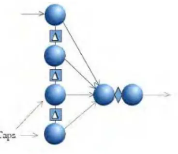
Figure 1. Finite Impulse Response Filter

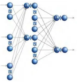
Figure 2 Multilayer Feedforward Neural Network

At each time increment, one new value is fed to input filters, and output neuron produces one scalar value. In effect this structure has the same functional properties as the Time Delayed Neural Networks (TDNN). However, the FIR neural network is interpreted as a vectoral and temporal extension of MLP. This interpretation leads to the temporal backpropagation algorithm.

3.2 Temporal backpropagation

The basic backpropagation algorithm assumes that the neural network is a combinational circuit, providing an output for a given input. However, many applications suitable for adaptive learning have inherently temporal structures.

Every time-delay neural network can be represented as a standard static network simply by duplicating nodes and removing delays. The resultant net is much larger, contains a large number of weight duplications (or triplications), and is not fully interconnected. The process of creating the static equivalent can be thought of as 'unfolding' the network. Once the network is unfolded, the backpropagation algorithm can be applied directly to solve the static network.

The output layer of the static network contains the same number of nodes as the output layer of the temporal network. Because this layer has no delay taps, the next layer has no non-physical nodes, and the number of virtual nodes of the static equivalent is equal to the number of filters in that layer times the number of placeholders in each filter. For each layer back to the input, the number of total virtual nodes is a cumulative sum of the number of virtual nodes in that layer plus the number of virtual nodes calculated for the previous layer minus one (because the first placeholder in each filter accepts and propagates its input without delay to the next layer). Mathematically, the notation for total virtual nodes at a layer is:















1

1

) 1 (l l l

T

T

T

L

l

L

l







1

where

T

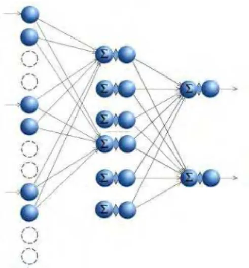
Figure 3. Partial static neural network in the unfolding process



   







n n t j l lin lijt

y

w





,

1

,

1









I

j

L

l

1

,

1









T

t

I

i

where l is used as a subscript to denote that there is only one tap s=1 associated with the output layer L. The network still has the exact physical layout of the temporal net, but without the delay units. The next step is to copy the first layer and second layer weights downward, overlapping placeholders when necessary, until the number of inputs in the first layer equals the number of accumulated inputs calculated.

4. Recurrent Neural Networks

A recurrent net is a neural network with feedback (closed loop connections). Examples include BAM, Hopfield, Boltzmann machine, and recurrent backpropagation nets. The architectures range from fully interconnected to partially connected nets, including multilayer feedfoward networks with distinct input and output layers. Fully connected networks do not have distinct input layers of nodes, and each node has input from all other nodes. Feedback to the node itself is impossible.

Two fundamental ways can be used to add feedback into feedforward multilayer neural networks. Elman introduced feedback from the hidden layer to the context portion of the input layer. This approach pays more attention to the sequence of input variables. Jordan recurrent neural networks use feedback from the output layer to the context nodes of the input layer and give more emphasis to the sequence of output values.

4.1 Learning in Recurrent Neural Networks

Hebbian learning and gradient ascent learning are key concepts upon which neural network techniques have been based. While backpropagation is relatively simple to implement, several problem can occur in its use in practical applications, including the difficulty of avoiding entrapment in local minima. The added complexity of the dynamical processing in recurrent neural networks from the time delayed updating of the input data requires more complex algorithms for representing learning.

Neural networks with recurrent connections and dynamical processing elements are finding increasing applications in diverse areas. While feedforward networks have been recognized to perform excellent pattern recognition even with complex nonlinear decision surfaces, they are limited to processing stationary patterns (invariant with time).

























))

(

(

)

(

)

(

)

(

)

(

)

(

)

(

k

v

k

y

j

k

v

k

w

i

k

u

k

w

k

v

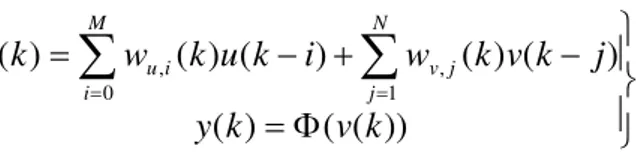
The transfer function of a neuron in a network using output feedback scheme can be expressed as:

























))

(

(

)

(

)

(

)

(

)

(

)

(

)

(

k

v

k

y

j

k

v

k

w

i

k

u

k

w

k

v

4.2 Recurrent Finite Impulse Response Neural Networks (RFIRNN)

Although variety of ANNs are used for time series prediction, there was no consensus on the best architecture to use. Horne and Giles [2] concluded that “recurrent networks usually did better than TDNNs except on the finite memory machine problem”. On the other hand Hallas and Dorffner [3] stated that “recurrent networks do not seem to be able to do prediction under the given conditions” and a “simple feedforward network significantly performs best for most nonlinear time series”. However, many agree that the best architecture is problem dependent and that efficiency of the learning algorithm is more important than the network model used.

Figure 4. Example of a three layer Recurrent FIR neural network

Not a lot of research has been done in time series modelling using RFIRNN. In RFIR, each feedback link has a non-zero delay, and the link between any two nodes has an explicit memory modelled by a multi-tap FIR filter for storing history information. (Figure 4) The advantage of this architecture is that it can store more historical information than both RNN and FIR. The concept of RFIR can be generalized easily to existing recurrent ANN, and nonlinear autoregressive networks. These networks use violation-guided backpropagation algorithm.

5. Performance Analysis

The coefficient of determination (C.D.) from Drossu and Obradovic [5] is used to compare the network’s forecasting performance:

The number of data points forecasted is n, xi is the actual value, x’i is the forecast value, and x’’ is the mean of the actual data. coefficient of determination close to one is preferable.

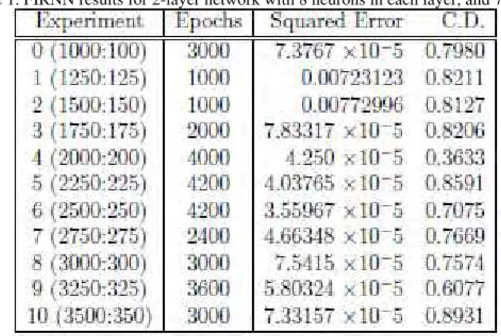
Below is a list of experiments which were performed on the two networks. Numbers 0-10 indicate level of difficulty, with 0 being shortest term prediction, and 10 longest. Numbers in form (A:B), are the number of training points (A) used for prediction, and the length of the horizon.

Table 1. FIRNN results for 2-layer network with 8 neurons in each layer, and 7:3 taps.

FIR training is an iterative process where each cycle consists of one or more forward propagations through the network, and one back propagation to obtain derivatives of the cost function with respect to the network weights. FIR networks used in this project have 2 hidden layers. Table 1 shows the results where the number of taps in first layer is 7, and 3 in second. The learning rate was set to 0.005 (same case for RNN performance in Table 2).

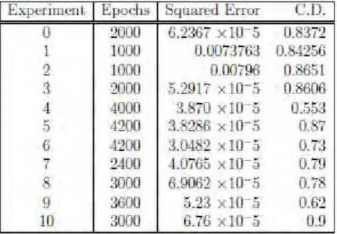
Table 2. RNN Results for 3-layer network with 10 neurons in each layer

Table 3. RNN Results for 3-layer network with 20 neurons in each layer

Common practice is to divide the time series into three distinct sets, training, testing, and validation sets. The training set is the largest set and is used by the network to learn the patterns present in the data. The testing set, ranging from 10% to 30% of the training set is used to evaluate the generalization ability of a supposedly trained network. The testing sets used in these examples are observations (series) which come after the training set, and had a size of 15% of training points. The size of the validation set must strike a balance between obtaining a sufficient sample size to evaluate a trained network and having enough remaining observations for both training and testing. The validation set thus consists of the most recent observations (last points of the training set). The validation set used in the experiments represented 10% of the training points.

The network is further trained until there is no improvement in the error function based on a reasonable number of randomly selected starting weights. Epochs columns in tables 1-4 show how many of them were needed for the network to converge.

By increasing the number of neurons in hidden layers, or tapped delays, more feautures are extracted from the data (and hence the predictions are made more accurate). However, this may lead to over-fitting, and the predictions might go out of range. Overfitting occurs when a forecasting model has too few degrees of freedom. In other words it has relatively few observations in relation to its parameters and therefore is able to memorize individual points rather than learn general patterns. To avoid this, either less epochs are used for training, or a very small learning rate is applied. Alternatively, one could linearly decrease the learning rate over time (decrease every 5-10 epochs), and use less epochs for training. Tables 3 and 4 show some improvement in the predictions, after the structure of the network has been expanded. In these experiments, the learning rate was reduced to 0.0025, and the number of epochs used for training has changed slightly in each experiment.

Sunspots

The sunspot time series have a higher degree of difficulty in time series prediction than Mackey-Glass, which is why more neurons need to be included in the network to do forecasting. When number of neurons per layer is less than 10, networks will perform poorly.

Two experiments were run on Sunspots, to forecast future 20, and 40 values (yearly values) using past 200 values. Research has shown that when predicting these dark blotches it is best to use yearly data rather than daily data (generally high frequency data is much harder to predict).

Before forecasting these series, preprocessing needs to be done. This is because the values of Sunspots are big for a neural network, and when forecasting, it is best to keep the values in range of [0,1]. Data normalization will fit the sunspots in the range of [0.1, 0.9]. Another preprocessing method which needs to be done is de-seasonalising, which will remove the trends found in sunspot numbers. [6]

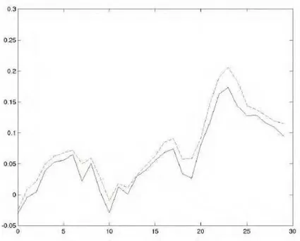
FIR network used for these experiments has 15 neurons in each layer, and 10:4 taps. RNN network has 25 neurons in each layer. Learning parameter was set to 0.03, and the number of training epochs was 2000. 0.03 was chosen as the parameter after careful testing. The RNN network outperformed FIR network in both experiment, significantly. The coefficient of determination in the first experiment was 0.44 for RNN, and 0.1 for FIR network. In the second experiment C.D. for the FIR network was nearly 0.

Figure 5. Comparison of RNN and FIRNN performance on sunspots prediction (left: FIRNN (C.D = 0.1), right RNN (C.D = 0.44)) (dotted lines denote predictions)

As mentioned before, the results showed that the RNN network outperformed the FIR network in the sunspot prediction. This might be due to the nature of sunspots. As mentioned earlier, sunspots usually rise and fal every 11.1 years, which acts as a threshold. Another predictive model, called Threshold Autoregressive (TAR) model, proposed by Tong and Lim [14] performs really well in this prediction task by employing a threshold to switch between two autoregressive models. The FIR model corresponds to the ARIMA (Autoregressive Integrated Moving Average) model, which when applied to sunspot prediction will converge to a local minimum due to the autoregressive feature (and the nature of sunspots). Momentum rate can be used to get pass the local minimum. After applying a momentum rate of 0.005, the following results were obtained for FIRNN:

The reason why RNN did not suffer as much as the FIR network is because it

does not have the autoregressive functionality as the FIRNN. Still, both networks performed below average (0.5), and TAR has shown to be a better predictive model for Sunspot prediction. One possible reason for the low performance of neural networks over TAR could be lack of training data.

5.2 S&P 500

The objective is to forecast future values of S & P 500 time series with the horizon set to 30 days. Whereas the objective may be to predict the level of the S&P 500, it is important to simplify the job of the network by asking for a change in the level rather than for the absolute level of the index.

The two architectures used in this project, FIR and RNN are both powerful forecasting tools. As mentioned earlier, in section 6, in order to capture more patterns, the architecture has to have a large number of neurons, or tapped delay connections. The networks which will be used for this experiment have 30 neurons in each hidden layer, with the FIR network having 10 taps in first layer, and 5 in second.

Training a neural network to learn patterns in the data involves iteratively presenting it with examples of the correct known answers. The objective of training is to find a set of weights between the neurons that determine the global minimum of the error function. Unless the model is overfitted, this set of weights should provide good generalization.

The objective is to forecast future 30 values of the S&P time series. The size of the training set is highly dependent on the value of this horizon. A big training set will contain points from which a large number of patterns will be extracted. The danger of this is the networks will learn too many patterns, and not be able to find correct future patterns due to a large number of choices.

A training set was selected for the experiment, containing 600 points (or days). The learning rate used in this experiment was 0.03, and the networks was trained for 10000 Epochs.

Coefficient of determination is 0.8 for the FIR network, whereas the RNN network performed slightly worse with a C.D. of 0.67. This is to be expected, as FIR networks perform better on short term prediction. This does not mean that the FIR network performs better in this task, because both networks have not been tested on a large dataset (long-term prediction).

6. Conclusion

Three different non-linear systems have been explored, and experimented upon. These include phenomena happening within the human body (Mackey-Glass), nature (Sunspots), and economics. Neural networks have shown to be a powerful forecasting tool. In order to do forecasting, networks must contain memory to learn the patterns which can be found in the data. There are two ways of doing this, either using FIR, or Recurrent neural networks. FIR neural networks outperform recurrent in short term prediction, whereas recurrent networks outperform fir networks on long term prediction.

Since FIR networks outperform RNN networks in short-term, and RNN outperform FIR in long term prediction, it seems reasonable to use a hybrid network, Recurrent FIR Neural Network for time series prediction. Such a network would have both the advantage of feedback connections of RNN networks, and FIR filters, which would in turn enable the network to learn more patterns than FIR and RNN combined together.

References

[1] Brock W. A. and Simon M. Potter. Nonlinear Time Series and Macroeconomics. G.S. Maddala, C.R. Rao, 1993. [2] Granger A. Forecasting stock market prices, a lesson for forecasters. International Journal of Forecasting, 1992. [3] Motley Fool Index Center. S&P 500. http://www.fool.com/school/indices/sp500.htm, 2004.

[4] D.Baily and D.M Thompson. Developing neural network applications. AI Expert, 1990.

[5] Drossu and Obradovic. Rapid design of neural networks for time series prediction. Computational Science and Engineering, [6] IEEE [see also Computingin Science & Engineering, Washington State Univ., 1996.

[7] Su Lee Goh and Danilo P. Mandic. Recurrent neural networks for prediction. Neural Networks, 2003.

[8] M. Hallas and G. Dorffner. A comparative study on feedforward and recurrent neural networks in time series prediction using [9] gradient descent learning. In R. Trappl, editor, Cybernetics and Systems 98, Proceedings of 14th European Meeting on [10] Cybernetics and Systems Research, Vienna, pages 644–647, 1998.

[11] Thomas Schreiber Holger Kantz. Nonlinear Time Series Analysis, 2nd edition. Cambridge University Press, 1997. [12] Horne and Giles. An experimental comparison of recurrent neural networks. Neural Information Processing Systems, MIT [13] Press, 1995.

[14] J.O.Katz. Developing Neural Network Forecasts for Trading. Technical Analysis of Stocks and Commodities, 1992. [15] Nikola K. Kasabov. Foundations of Neural Networks, Fuzzy Systems, and Knowledge Engineering. MIT Press, 1996. [16] C.C. Klimasauskas. Neural Networks in Finance and Investing: Using Artificial Intelligence to improve real performance. [17] R.R. Trippi and E.Turban, Chicago, 1993.

[18] O.Ersoy. Neural Network Tutorial. Hawaii International Conference on System Sciences, 1990.

[19] H. Tong and K.S. Lim. Threshold Autoregression, limit cycles, and cyclical data. J Roy Statisti Soc, 1980.

[20] Benjamin W. Wah and Minglun Qian. Constrained-Based Neural Network Learning for Time Series Prediction. University [21] of Illinois, Urbana Champaign, USA, 2001.

Appendix A