F
ACULDADE DEE
NGENHARIA DAU
NIVERSIDADE DOP
ORTODevelopment of a Servo Motor
Optimised for Robotic Applications
João David Soares Silva
Mestrado Integrado em Engenharia Eletrotécnica e de Computadores Supervisor: Paulo José Cerqueira Gomes da Costa
Second Supervisor: José Alexandre Carvalho Gonçalves
Abstract
Servo motors are actuators that allow for position control. They consist of a DC motor coupled to a reduction gearbox, a position feedback sensor and the electronic circuit responsible for de-coding the pulse width signal reference and driving the motor itself. They move from one position to another nearly at maximum speed which can cause abrupt movements and current spikes in the power supply. By using potentiometers as position sensors, they offer a narrow sense range and usually can’t be used in continuous rotation mode. For that reason, most can only position the motor shaft between 0◦and 180◦.
SMORA (Servo Motor Optimised for Robotic Applications) consists of custom hardware and firmware that includes a microcontroller and a series of sensors, allowing for the motor’s current, temperature and voltage to be measured in real-time, as well as precise position feedback thanks to the included hall-effect magnetic position encoder. It also includes an accelerometer and a gy-roscope to measure the servo’s body relative position and rotation.
This thesis focuses on the development of SMORA from a hardware, firmware and software perspective. The implemented hardware and communication protocol will be described and the PID and speed compensation algorithms used for the control explained and demonstrated.
Acknowledgements
I would like to start by thanking my advisor Paulo Costa for his constant support, availability and dedication, as well as experience and advise. He was the main proponent for this thesis. Also to my co-advisor José Gonçalves for his helpful tips and support.
This work would not have been possible without the constant support of friends and family. To the Harding, Silvéria and Mason family, who were personally invested in the success of this thesis. To the Goldstraw family who day in and day out supported me and my quirks. To all the Riverside family, who’s constant prayer and encouragement were invaluable. To my parents for giving me this priceless opportunity. Thank you all for your friendship and support.
Thank you Fia for all this years of patience, endurance and loyalty. Thank you Lord.
João Silva
“A wise man will hear and increase learning, And a man of understanding will attain wise counsel”
Proverbs 1:5
Contents
1 Introduction 1 1.1 Context . . . 1 1.2 Motivation . . . 2 2 Literature Review 3 2.1 Controller Architecture . . . 3 2.1.1 PID . . . 3 2.1.2 PIV . . . 4 2.1.3 Feed-Forward . . . 5 2.2 Parameter Estimation . . . 6 2.3 Existing hardware . . . 8 2.3.1 Open Servo . . . 8 2.3.2 SuperModified . . . 8 2.3.3 Moti . . . 9 2.3.4 AX-12A . . . 9 2.4 Conclusion . . . 10 3 Implementation 11 3.1 Hardware . . . 11 3.1.1 MG996R Reverse engineering . . . 12 3.1.2 Magnetic Encoder . . . 13 3.1.3 EEPROM . . . 133.1.4 MPU-6050 accelerometer and gyroscope . . . 14
3.1.5 Magnetic encoder: voltage regulation and translation . . . 14
3.1.6 Position encoder PCB . . . 15
3.1.7 Temperature sensor . . . 16
3.1.8 Current and voltage sensor . . . 16
3.1.9 Half-duplex interface . . . 17
3.1.10 Motor driver . . . 18
3.1.11 RGB Led . . . 19
3.1.12 Power supply regulation and protection . . . 19
3.1.13 SMORA Variants . . . 20
3.1.14 External cover 3D model . . . 22
3.1.15 SMORA prototype . . . 23 3.1.16 BOM list . . . 24 3.2 Software . . . 25 3.2.1 Bootloader . . . 25 3.2.2 Communication Protocol . . . 25 vii
viii CONTENTS
3.2.3 Host side software . . . 27
3.2.4 Arduino firmware . . . 27 3.3 Algorithms . . . 29 3.3.1 PID equation . . . 29 3.3.2 Position PID . . . 30 3.3.3 Speed compensator . . . 32 3.3.4 Speed PID . . . 35
4 Conclusion and future work 37 4.1 Goal accomplishments . . . 37
4.2 Future work . . . 39
A 41
List of Figures
1.1 RC Servo disassembled showing its main elements [1] . . . 1
2.1 Basic PID Controller . . . 4
2.2 Basic PIV Controller . . . 5
2.3 Basic Feed-Forward Controller . . . 6
2.4 DC motor equivalent circuit . . . 6
2.5 Open servo V3 circuit . . . 8
2.6 SuperModified v3.0 circuit . . . 8
2.7 Moti servomotor . . . 9
2.8 Robotis AX-12A smart servo motor [2]. . . 9
3.1 Simplified diagram of a servo motor . . . 11
3.2 SMORAs diagram . . . 12
3.3 3D rendering of the inside of a MG996R servo enclosure, magnet holder and shaft. 13 3.4 AS5048B. . . 13
3.5 24LC16BT circuit schematic . . . 14
3.6 MPU-6050. . . 14
3.7 Position encoder supply and level translator. . . 15
3.8 3D rendering of the position encoder PCB. . . 15
3.9 Position encoder PCB prototype. . . 16
3.10 Temperature sensor. . . 16
3.11 Current and voltage sensor schematics. . . 17
3.12 Half-duplex connectors schematic. . . 17
3.13 Half-duplex circuit. . . 18
3.14 Motor driver. . . 18
3.15 RGB LED schematic. . . 19
3.16 Power supply schematic. . . 19
3.17 Actual picture of the 2ndprototypes of SMORA-A32 to the left and SMORA-A8 to the right. . . 20
3.18 USB-to-Serial interface schematic. . . 20
3.19 Half-duplex programmer’s schematic. . . 21
3.20 SMORA-A8 programmer and half-duplex interface prototype. . . 21
3.21 Actual picture of SMORA-A32 final PCBs manufactured by OSHPark. . . 21
3.22 TXS0101 schematic. . . 22
3.23 3D rendering of the SMORA PCB variants. . . 22
3.24 3D rendering of SMORA A32 cover . . . 23
3.25 SCARA elbow. . . 23
3.26 Pictures of the final SMORA-A32 prototype. . . 24
x LIST OF FIGURES
3.27 SMORA-A8 ICSP. . . 25
3.28 Half-duplex transmitted frame at 1Mbit/s. . . 26
3.29 Half-duplex received status frame at 1Mbit/s. . . 26
3.30 Oscilloscope view of the half-duplex communication at 1Mbit/s. . . 27
3.31 Diagram of the position PID. . . 30
3.32 Position PID step-response with different gains. . . 30
3.33 Position PID step-response to different position commands. . . 31
3.34 Present speed with a speed command of 200◦/s. . . 32
3.35 Present speed vs angle with a speed command of 200◦/s. . . 32
3.36 Hammerstein model. . . 33
3.37 Plot of multiple speeds compensated. . . 33
3.38 Polar plot of multiple speeds compensated. . . 34
3.39 Diagram of the speed PID. . . 35
3.40 Speed PID step-response. . . 35
3.41 Speed PID step-response to different speed commands. . . 36
A.1 Position encoder full schematic . . . 41
A.2 SMORA-A8 main board schematic. . . 42
A.3 SMORA-A32 main board schematic. . . 43
A.4 SMORA-A8 programmer and interface circuit schematic. . . 44
A.5 Position encoder board. . . 45
A.6 SMORA-A8 programmer board. . . 45
A.7 SMORA-A8 board. . . 46
A.8 SMORA-A32 board. . . 46
List of Tables
3.1 Sensor timing . . . 28
A.1 Speed compensation array . . . 48
A.2 SMORA-A8 main PCB BOM list as of January, 2017. . . 49
A.3 SMORA-A8 encoder PCB BOM list as of January, 2017. . . 49
A.4 SMORA-A32 main PCB BOM list as of January, 2017. . . 50
A.5 SMORA-A32 encoder PCB BOM list as of January, 2017. . . 50
Abbreviations
ADC Analog to Digital Converter API Application Programming Interface BOM Bill of Materials
CDC Communication Device Class DC Direct Current
DMP Digital Motion Processor DXF Drawing Exchange Format
EEPROM Electrically Erasable Programmable Read-Only Memory I2C Inter-Integrated Circuit
IC Integrated Circuit
ICSP In-Circuit Serial Programming LDO Low-Dropout
LED Light Emitting Diode
MEMS Micro-Electro-Mechanical Systems
MOSFET Metal Oxide Semiconductor Field Effect Transistor PCB Printed Circuit Board
PID Proportional Integral Derivative PIV Proportional Integral Velocity PWM Pulse-Width Modulation QFN Quad Flat No leads RC Radio Controlled RGB Red Green Blue RTS Ready-to-Send
SCARA Selective Compliance Articulated Robot Arm SCL Serial Clock Line
SDA Serial Data Line
SMORA Servo Motor Optimised for Robotic Applications SRAM Static Random Access Memory
STL STereoLithography SWD Serial Wire Debug TWI Two Wire Interface
UART Universal Asynchronous Receiver/Transmitter USB Universal Serial Bus
Chapter 1
Introduction
This chapter will give a context to RC servo motors in robotic applications as well as explain the motivation for creating an improved version.
1.1
Context
Figure 1.1: RC Servo disassembled showing its main elements [1]
A servo motor (Fig.1.1) is a rotary/linear actuator, the purpose of which is to allow precise control of angular/linear position. It is comprised of a DC motor coupled with a reduction gear system and a position feedback sensor for closed-loop control. Although sometimes employed in industrial applications, their most common use case is in radio-controlled models such as planes and cars. These RC servo motors are distinct from the industrial type mostly by their lower torque, size and cost and more basic interface capabilities.
Their ease of use, high torque quality, convenient package and low price allow for a wide adoption in the field of robotics. Tasked to move and maintain itself at a particular position,
2 Introduction
most servos have a range from 0◦ to 180◦ when unmodified. By their self-integrated nature, they eliminate the need to: design a control system; analyse the transient response; fine tune the feedback loop; determine the proper gear ratio for a specific speed and efficiency; choose an appropriate motor; build the amplifier and motor driver.
Servo motors generally have three connection wires: power, ground and signal. The signal line is fed with a PWM signal (pulse width modulation). The width of the pulse is then used to determine the angle to which the device should move. A short one millisecond pulse sets it to 0◦ while a longer two millisecond pulse sets it to 180◦.
1.2
Motivation
Even though servos have excellent qualities when used in the field of robotics, several prop-erties can still be enhanced. These devices are known to have nonlinear propprop-erties and dynamic factors such as dead-zones, backlash and friction that might hinder their precision and accuracy. They usually do not provide position, velocity or current feedback to the device controlling them. Factors such as a change in the load attached to the system increase the complexity of the analysis even further. Controlling these servos using a PWM signal might also become complicated if the number of servo motors to control increases.
The intent of this thesis is to rebuild a servo motor comprising several sensors and higher level addressing/communication capabilities. Also studying it’s characteristics through experimental analysis.
Chapter 2
Literature Review
In this chapter, some methods for model parameter extraction necessary for an accurate control of the DC motor, controller architectures, as well as existing hardware which deploy some of these technologies will be reviewed.
2.1
Controller Architecture
When choosing a servo motor, it is important to have a good understanding of the system to be controlled. The better that knowledge, the higher the chances of accomplishing a desired behaviour. However, the control algorithm is paramount to the improvement of transient response times and reduction of steady state errors and sensitivity to load parameters.
Servo control can generally be broken down into two classes of problems [3]: Command tracking and disturbance rejection. The first pertains to how well the actual motion follows the position, velocity, acceleration and torque commands. The second, can include anything from torque disturbance on the motor shaft to supply voltage variations.
PID (Proportional Integral and Derivative)2.1.1and PIV (Proportional Integral and Velocity)
2.1.2loops are the most common controller strategies employed. Unlike Feed-Forward control, which can anticipate the internal commands for zero error following, disturbance rejection reacts to unknown disturbances and modelling errors. To improve the overall performance, both of these control types can be combined.
2.1.1 PID
The typical servo motion controller topology is depicted in Fig.2.1. G(s) represents the DC motor driver transfer function.
The servo drive receives a signal command that represents a motor current. The following equation relates motor shaft torque T with motor armature current I by a torque constant factor Kt (2.1).
T = KtI (2.1)
4 Literature Review
The parameters for the motor are the rotor and load moment of inertia J, viscous friction constant (dampening) b and torque constant factor Kt. The actual position θ (s) can be measured by an encoder coupled to the motor shaft. Td models the load disturbance while θr(s) represents the desired position command.
Kp Ki s s Kd ∑ (s) θr ∑ -Kt ∑ Js1 1s b -PID Servo Drive Servo Motor Td θ(s) ω(s) G(s)
Figure 2.1: Basic PID Controller
The PID operates on the position error and outputs a torque command to the servo driver. Three gains need to be adjusted in the PID controller (Kp, Ki and Kd). They act on the error between desired and present position (2.2).
e(t) = θr(s) − θ (s) (2.2)
The signal output from the PID is2.3.
u(t) = Kpe(t) + Ki
Z
e(t)δ t + Kd d
dte(t) (2.3)
There are two main ways of selecting the gains for the PID controller. Trial-and-error based on the operators own experience or an analytical approach. The first has the downside that there is no physical insight into what the gains mean or even if they are optimal. The second can be accomplished by, for example, following Ziegler and Nichols [4] [5] method based on setting Ki and Kd to zero, analysing the system’s step response while slowly increasing Kp until the shaft position oscillates and recording both Kp and the oscillation frequency. That data can then be used to calculate the final values of Kp, Kiand Kd. This last approach doesn’t usually yield many benefits to a high-performance system. The settling time can generally be further improved.
2.1.2 PIV
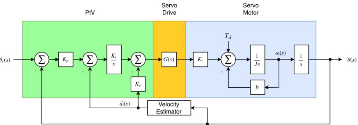
An easier to tune alternative to the PID that has a better to predict system response is the PIV topology (Fig.2.2). This controller combines a position and velocity loop. A velocity correction command results from the position error multiplied by Kp. Kinow operates directly on the velocity error as opposed to the position error in the PID. Kdis replaced by Kv.
2.1 Controller Architecture 5 Kt ∑ 1 Js 1s b -PIV Servo Drive Servo Motor Td θ(s) ω(s) G(s) Kv Ki s ∑ ∑ - -∑ -Velocity Estimator (s) ω̂ Kp (s) θr
Figure 2.2: Basic PIV Controller
To accurately use this topology, a good knowledge of the motor velocity is required. To tune this system, two control parameters are needed: The bandwidth(BW) and damping ratio(ζ ). An estimate of the rotor and load moment of inertia ˆJ and damping constant ˆb are also required. Higher bandwidth is related to quicker rise and settling times while damping pertains mainly to overshoot. The Kp, Kiand Kvconstants can be calculated from equations2.4,2.5and2.6.
Kp= 2πBW 2ζ + 1, (s −1) (2.4) Ki= (2πBW )2(1 + 2ζ ) ˆJ, (N m rad−1) (2.5) Kv= (2πBW )((1 + 2ζ ) ˆJ) − ˆb, (N m rad−1s) (2.6) 2.1.3 Feed-Forward
To accomplish near zero following and tracking errors, Feed-Forward is often used in combi-nation with a PID or PIV loop. For this topology, the controller needs access to a position θr(s), velocity ωr(s) and acceleration αr(s) commands (Fig.2.3). Total inertia ˆJ and damping ration ˆb estimates should also be available.
To calculate the estimated torque needed to make the desired motion, equation2.7is used.
U(s) = ˆJ(αr(s)) + ˆb(ωr(s)) (2.7) Feed-Forward control reduces settling time and minimizes overshoot. In any case, to increase the velocity estimation accuracy, an encoder with enough resolution for the feedback is also re-quired.
6 Literature Review b̂ ∑ Ĵ (s) ωr (s) αr Feed-Forward Kp Ki s s Kd ∑ (s) θr ∑ -Kt ∑ 1 Js 1s b -PID Servo Drive Servo Motor Td θ(s) ω(s) G(s) ∑ s s
Figure 2.3: Basic Feed-Forward Controller
2.2
Parameter Estimation
RC servo motors are comprised of three main components: a DC motor, driving circuitry with potentiometer encoder for position feedback and gear reduction system. When modelling the controller, certain parameters from the DC motor need to be appropriately measured or estimated for an improved control [6]. They can be extracted from the transitory response to a step on the input and steady state response for different input voltages [7]. The model in Fig.2.4 can be defined by equation 2.8, where ia is the armature current and the voltage V is the sum of the voltage drop across the equivalent resistance R, equivalent inductance L and back electromotive force e. V = Ria+ L ∂ ia ∂ t + e (2.8)
V
θ
J
b
θ˙ T
+
ce
= Kθ˙
Td
R
L
ia
Figure 2.4: DC motor equivalent circuit
Equation 2.9 shows the resulting torque Tr as it relates to the developed torque Td, static friction torque Tc and viscous friction b ˙θ .
2.2 Parameter Estimation 7
The following equations express the relationship between developed torque Tdand current ia (2.10), back electromotive force e and angular velocity ω (2.11) and load torque TLwith moment of inertia J and angular acceleration ˙ω (2.12).
Td= Kia (2.10)
e= Kω (2.11)
TL= J ˙ω (2.12)
From this equations we can obtain the angular acceleration ˙ω (2.13) which can then be discre-tised into2.14where 4T is the sampling time.
˙
ω = Kia− Tc− bω
J (2.13)
ω [k] = ω [k − 1] + 4TKia[k − 1] − Tc− bω[k − 1]
J (2.14)
Equation2.15can then be attained by minimising the sum of the absolute error between the estimated (2.14) and actual transitory response, assuming zero inductive voltage drop across L and initial known values of Tcand K.
J ˙ω = K R(V − Kω) − bω − Tc (2.15) Solving2.15yeilds2.16: ω (t) = c d(1 − e −dt) (2.16) where: c=KV− RTc RJ (2.17) d=K 2+ Rb RJ (2.18)
In steady state ω =dc resulting in:
ω = K
K2+ RbV− RTc
K2+ Rb (2.19)
By repeating the procedure starting from an estimated value for R to obtain Tc and K and replacing them with the new estimations to get R back, the parameters will converge to the real values.
8 Literature Review
2.3
Existing hardware
There are already several smart servo motors which include an array of sensors and commu-nication protocols that attempt to shorten the prototyping phase by giving the designer tools to aid the process and increase development efficiency and speed.
2.3.1 Open Servo
First presented in 2005, Open Servo [8] was an attempt to develop an open community-based project with the goal of creating a drop-in replacement digital servo controller for robotics. In it’s 3rdrevision (Fig.2.5), the circuit boasts features such as speed and temperature sensing, indepen-dent H-bridge allowing for breaking, ATMega168 at 20MHz, 400khz I2C/TWI interface, 6V to 7.5V voltage input and 3A continuous current output. But the angle of rotation is still bound by the limits of the mechanical potentiometer. It seems that for the last few years it’s development has abated.
Figure 2.5: Open servo V3 circuit
2.3.2 SuperModified
The SuperModified v3.0 [9] (Fig.2.6) circuit offers a complete DC motor controller. Like the Open Servo, it’s designed to fit inside of a regular RC servo motor. The circuit includes a 15-bit absolute position encoder, continuous 360◦range, position and velocity profiled movements, mul-tiple bus interfaces such as RS-485, UART and I2C and 5V to 24V voltage input at 5A continuous current output.
However, the hardware and firmware are proprietary, thus preventing the development com-munity from improving it’s functionality. Depending on the application, it’s cost of 55e might prove uneconomical considering that a servo to apply it to also needs to be purchased.
2.3 Existing hardware 9
2.3.3 Moti
Appearing for the first time at the end of 2014, Moti [10] (Fig.2.7) promised to be a "smart servo motor that makes it easier to build robots". Like Open Servo and SuperModified, Moti aims to be a drop-in replacement to the typical controller. The major difference being that the developer wanted it to "play well with the web and mobile devices, so there’s a RESTful API for developing apps".
Unfortunately Moti is still not available to the public after an unsuccessful Kickstarter cam-paign and it doesn’t seem like the hardware and firmware will be open-source.
Figure 2.7: Moti servomotor
2.3.4 AX-12A
The Robotis AX-12A [11] (Fig.2.8) "is the most advanced actuator on the market in this price range and has become the defacto standard for the next generation of hobby robotics"[2]. By including a half-duplex asynchronous serial communication interface with 1Mbit baud rate, this servo has the ability to track its position, speed, temperature, voltage and load while allowing for the strength and speed of the motor’s response to be controlled. It’s enclosure is designed so that various robot forms can be accomplished through the use of specially designed frames that allow multiple devices to be mechanically linked together.
Nevertheless, the limitations of a mechanical position sensor are still present. Despite having a larger position sense range when compared to most RC servo motors, there is yet a 60◦ dead-zone where the position is unknown. Like the SuperModified, the hardware and firmware are proprietary.
10 Literature Review
2.4
Conclusion
Disturbance rejection can be obtained from PID and PIV controllers. Because the overshoot and rise times are tightly coupled, a change in any of the gains greatly influences the overall system. PIV control provides for a decoupled management of overshoot and rise times, while allowing easier tuning and high disturbance rejection qualities. Feed-forward helps to mitigate tracking errors.
Parameter estimation can be accomplished by extracting the transitory response to a step on the input and steady state response for different input voltages. By starting from an initial set of estimations, R, Tcand K can be further iterated to converge to their true values.
Chapter 3
Implementation
RC servo motors allow for position control. However, they move from one position to another at maximum speed which can cause abrupt movements and current spikes in the power supply. By using potentiometers as position sensors, they offer a narrow sense range and their resolution is limited by the ADC responsible for reading their voltage output. For that reason, most can only position the motor shaft between 0◦ and 180◦. Fig.3.1 shows a simplified diagram of a typical servo motor. Motor Setpoint Output shaft Potentiometer Position feedback Electronics Gearbox
Figure 3.1: Simplified diagram of a servo motor
Certain modifications can be performed, such as removing the limit pin from the output shaft. Nonetheless, the movement is still constrained by the mechanical range of the potentiometer itself. Furthermore, there is no feedback on the present position so the user can only guess where the shaft actually is.
This chapter will describe the design process for SMORA from a hardware and software per-spective.
3.1
Hardware
SMORA is an open-source attempt at sidestepping the shortcomings of previous devices while adding more features at a similar price range. By replacing the mechanical potentiometer with a hall-effect magnetic encoder, SMORA allows for high resolution position and speed feedback while having true 360◦rotation capabilities. Additionally, it includes current, voltage, temperature
12 Implementation
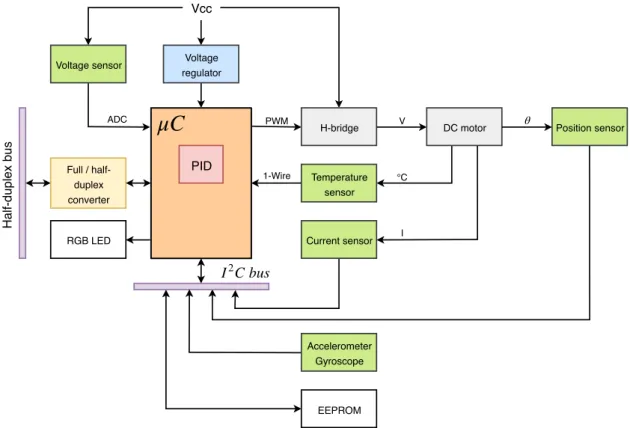
and attitude sensors. Not only can a user retrieve their data through the included half-duplex serial interface but also use them to build new algorithms and features that the other devices are not capable of, such as retrieving the present yaw, pitch and roll of the device itself. By taking advantage of the original MG996R metal gears, SMORA is more rigid and endures higher loads without breaking. Voltage regulator H-bridge Vcc DC motor PWM V Position sensor θ H a lf -d u p le x b u s Current sensor Temperature sensor 1-Wire C bus I2 Accelerometer Gyroscope Full / half-duplex converter RGB LED EEPROM Voltage sensor ADC °C I
μC
PIDFigure 3.2: SMORAs diagram
Fig.3.2shows the diagram of the architecture chosen to base the development of the circuit on.
3.1.1 MG996R Reverse engineering
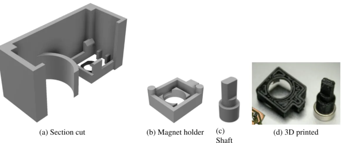
The development of the SMORA prototype started with reverse engineering a MG996R servo motor. The inner dimensions were measured with a digital caliper and used to build a simplified 3D model of the inside (Fig.3.3a). As the selected position sensor needs a diametrically magnetised neodymium magnet, to hold it in place and keep it centered while the shaft rotates, two additional models were created (Fig.3.3band Fig.3.3c). With the dimensions constrained, a DXF file with the outline for the magnetic encoder PCB was exported.
3.1 Hardware 13
(a) Section cut (b) Magnet holder (c) Shaft
(d) 3D printed
Figure 3.3: 3D rendering of the inside of a MG996R servo enclosure, magnet holder and shaft.
3.1.2 Magnetic Encoder
Unlike most of the RC servo motors commonly available, to measure the shaft position SMORA uses a AMS AS5048B [12] hall-effect magnetic encoder instead of a potentiometer. It works by measuring the magnetic field of a diametrically magnetised neodymium magnet (Fig.3.4b) and calculating it’s angle of rotation. With 14-bit resolution provided through I2C, this sensor is capa-ble of outputting 16384 positions per revolution while allowing for a full 360◦rotation (Fig.3.4a). To that end, the limit pin from gearbox output gear had to be removed (Fig.A.9).
(a) Schematic. (b) Magnet diagram. Figure 3.4: AS5048B.
3.1.3 EEPROM
To allow for some flexibility, and considering that some microcontrollers don’t have an internal EEPROM, SMORA includes an external Microchip 24LC16BT 2Kbyte EEPROM [13] (Fig.3.5). This memory can be used to store, for example, configuration parameters such as PID gains and position, speed and alarm limits.
14 Implementation
Figure 3.5: 24LC16BT circuit schematic
3.1.4 MPU-6050 accelerometer and gyroscope
SMORA is the only servo that allows the user to get feedback on the devices attitude. A InvenSense MPU-6050 [14] (Fig.3.6aand 3.6b) containing a 16-bit MEMS accelerometer and gyro can give feedback on the pitch, roll and yaw (Fig.3.6c), either by supplying the raw data or by using the integrated DMP (Digital Motion Processor) to calculate it.
(a) Schematic.
(b) QFN IC. (c) Axes. Figure 3.6: MPU-6050.
3.1.5 Magnetic encoder: voltage regulation and translation
To allow the magnetic encoder PCB to operate at either 3.3V or 5V supplies and interface logic levels, a MIC5219-3.3 LDO voltage regulator [15] (Fig.3.7a) was added, as well as two BSS138 N-channel MOSFETs [16] acting as voltage translators (Fig.3.7b) for the SDA and SCL lines.
3.1 Hardware 15
This level shifting is necessary if the host and master operate at different voltages, lest the device with the lower supply has a voltage on it’s lines higher than it tolerates, potentially damaging it.
(a) 3.3V voltage regulator schematic (b) Level translator schematic Figure 3.7: Position encoder supply and level translator.
Jumpers J1, J2 and J3 should be shorted to configure it to operate at 3.3V. In that case, the BSS138 MOSFETs and MIC5219-3.3 LDO voltage regulator can be omitted.
3.1.6 Position encoder PCB
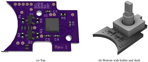
A 3D model of the position encoder PCB was created to test the fitting against the initial 3D model before being fabricated (Fig.3.8aand Fig.3.8b).
(a) Top. (b) Bottom with holder and shaft. Figure 3.8: 3D rendering of the position encoder PCB.
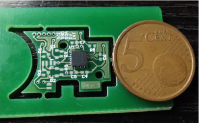
Fig.3.9shows a picture of the position encoder PCB with the MPU-6050 accelerometer/gyro populated next to a 5 cent coin for size comparison.
16 Implementation
Figure 3.9: Position encoder PCB prototype.
3.1.7 Temperature sensor
In order to preserve the proper operation of the DC motor, the temperature needs to be mon-itored and kept below a certain level. To that end, a Maxim DS18B20 [17] (Fig.3.10a) 9-bit to 12-bit resolution digital thermometer is adjoined to it by thermal paste (Fig.3.10b) and communi-cates over a 1-Wire bus, thus requiring only one data line. It is powered from the same source as the microcontroller although the sensor itself can derive power directly from this data line ("para-sitic power"). Providing an alarm function with non-volatile user-programmable upper and lower points allows for the microcontroller to offload the over-temperature triggering.
(a) Schematic. (b) Adjoined to the motor. Figure 3.10: Temperature sensor.
3.1.8 Current and voltage sensor
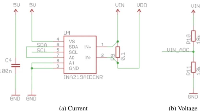
Having the ability to measure the motor current allows for it’s different parameters and torque to be estimated. Torque limitation and control can also be accomplished. A Texas Instruments
3.1 Hardware 17
INA219A [18] (Fig. 3.11a) is used to monitor the motor’s current through a 0.1 ohm shunt re-sistor. This sensor reports shunt voltage drop, bus supply voltage and power with programmable conversion times and filtering. It enables direct current readouts in milli-Amperes and voltage in Volts through the I2Cinterface.
Additionally, the power supply voltage can also be monitored through a resistive voltage di-vider connected to an ADC pin (Fig.3.11b).
(a) Current (b) Voltage
Figure 3.11: Current and voltage sensor schematics.
3.1.9 Half-duplex interface
SMORA connects to the outside world through a half-duplex serial interface. As opposed to full-duplex, it is devised to only transmit or receive at a time. However, it only requires one line instead of two.
The same cable is used for communication and power. The Molex PicoLock 4 pin connectors allow for up to 3A of supply current. Multiple SMORA’s can be daisy-chained together (Fig.3.12) and communicate at speeds of over 1Mbit/s.
18 Implementation
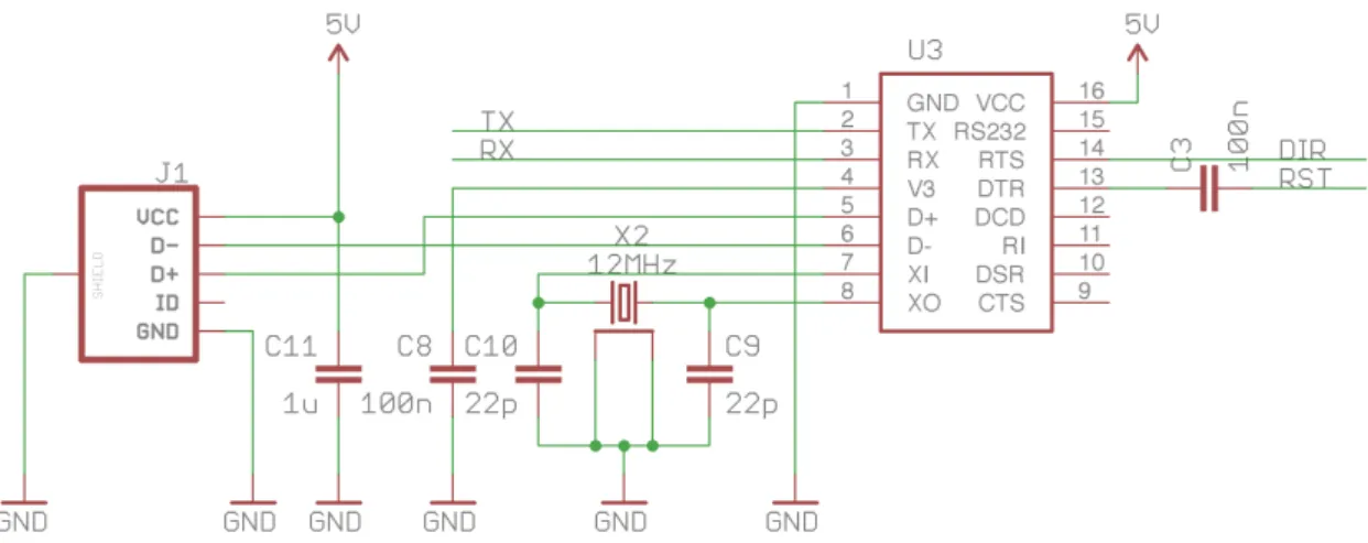
A Texas Instruments SN74LVC2G241 [19] (Fig. 3.13) dual-buffer and driver with tri-state outputs is responsible for integrating the half-duplex interface and the full-duplex serial interface of the microcontroller.
(a) Schematic. (b) Diagram.
Figure 3.13: Half-duplex circuit.
By controlling the output-enable inputs of the buffers, the microcontroller can regulate which pin of the full-duplex serial interface (receive or transmit) should be connected to the half-duplex data pin. Setting the DIR pin high will enable transmission while setting it low enables reception. A 100 ohm resistor in series with the data line is used to limit the buffers current, lest there is a collision if multiple devices try to transmit at the same time.
When the buffers are disabled, their output are in high impedance. To assure that the RX line stays at a logic high level when this happens, a 10K resistor pull-up was added. Similarly, a pull-up resistor in the DIR line guarantees that it stays at a known logic level while the microcontrollers’ pins are being configured during startup.
3.1.10 Motor driver
The Texas Instruments DRV8835DSSR [20] (Fig. 3.14a) is an integrated dual low-voltage H-bridge capable of up to 3A drive current (when both H-bridges are connected in parallel).
(a) Schematic. (b) WSON-12 IC packaging. Figure 3.14: Motor driver.
3.1 Hardware 19
It operates on a motor supply from 0V to 11V and a device supply from 2V to 7V. The mi-crocontroller uses this driver to control the motor’s torque using a PWM signal and a direction signal. This driver was mainly chosen for it’s ultra-compact WSON form-factor (Fig.3.14b) and for having a current supply capability above what the motor requires. This current was measured to be below 2A with the DC motor shaft locked.
3.1.11 RGB Led
To show the user if there is an alarm situation, SMORA employs a common-cathode RGB LED (Fig.3.15). This LED is also used for the bootloader status.
Figure 3.15: RGB LED schematic.
3.1.12 Power supply regulation and protection
SMORA can be powered from 5V to 11V (versus 9V to 12V of the AX-12A) through the half-duplex interface cable. A MIC5219-5V [15] LDO regulator is employed to regulate this voltage down to 5V while a high-side DMP3099L-7 [21] P-channel MOSFET protects the circuit from reverse polarity [22] (Fig.3.16a). A 47uF ceramic capacitor ensures that the supply stays as noise-free as possible.
(a) Regulation and reverse-polarity protection. (b) Voltage selector. Figure 3.16: Power supply schematic.
20 Implementation
Additionally, due to SMORA being programmable through an external interface (USB or se-rial) that can also power it, a FDN340P P-channel MOSFET (Fig.3.16b) ensures that only one power supply is connected at a time. Priority is given to the power received from the half-duplex interface cable.
3.1.13 SMORA Variants
SMORA comes in two variants: SMORA-A8 and SMORA-A32 (Fig.3.17).
Figure 3.17: Actual picture of the 2ndprototypes of SMORA-A32 to the left and SMORA-A8 to the right.
SMORA-A8 (full schematic in Fig.A.2) includes a 8-bit ATmega328p with 32KB of flash memory and 2KB of SRAM running at 5V and 16MHz. It was chosen in this variant for being hugely popular amongst the developer and maker community. The amount of open-source project created with this microcontroller translates into a wealth of information when it comes to available source-code and hardware designs. Thus, allowing for faster firmware development.
Figure 3.18: USB-to-Serial interface schematic.
To program the SMORA-A8 variant, a USB-to-Serial interface was created based on the CH340G integrated circuit (Fig. 3.18). A SN74LVC2G241 [19] was also included that allows
3.1 Hardware 21
the same board to both program and interface with the half-duplex bus with the communication direction managed by a computer through the CH340G RTS pin (Fig.3.19).
Figure 3.19: Half-duplex programmer’s schematic.
The final programmer prototype is shown in Fig.3.20and it’s full schematic in Fig.A.4.
(a) Top. (b) Bottom.
Figure 3.20: SMORA-A8 programmer and half-duplex interface prototype.
SMORA-A32 (Fig.3.21) includes a 32-bit ATSAMD21G18A ARM Cortex-M0+ with 256KB of flash memory and 32KB of SRAM running at 3.3V and 48MHz with a 32.768KHz crystal. Having 8 times more flash, 16 times more RAM and thrice the speed, allows this microcontroller to include more complex algorithms than it’s ATmega328p counterpart.
22 Implementation
The SMORA-A32 variant can be programmed directly through the included USB interface. When plugged into a computer, it presents a CDC serial interface capable of speeds of over 2.5Mbit/s that can also be used for debugging and to allow it to act as a master in the half-duplex bus network. A resettable fuse protects the circuit from currents over 500mA through the USB port.
A MIC5219-3.3V [15] LDO regulator is employed to regulate the voltage down to 3.3V. To ensure that the half-duplex bus always runs at 5V, a Texas Instruments TXS0101 [23] (Fig.3.22) 1-bit bidirectional voltage level translator is included.
Figure 3.22: TXS0101 schematic.
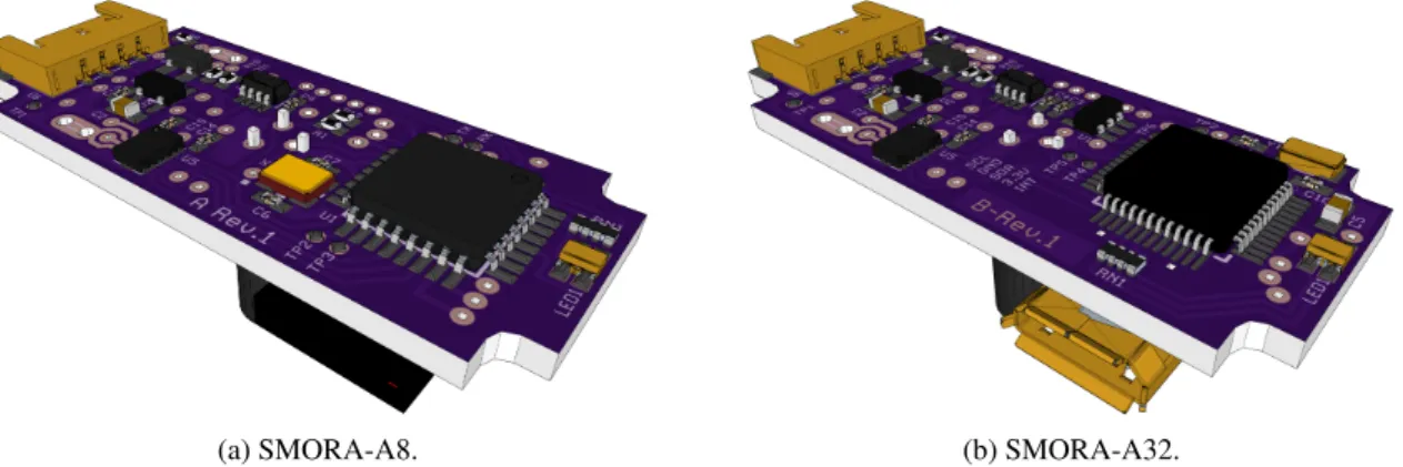
3.1.14 External cover 3D model
Because SMORA’s custom PCB is larger than the one used in a MG996R servo, in order for the device to be self contained a custom 3D cover model was designed. To ensure the PCBs would fit, they were first modelled in 3D (Fig. 3.23a and Fig.3.23b) so that a cover could be created around them (Fig.3.24).
(a) SMORA-A8. (b) SMORA-A32.
3.1 Hardware 23
Figure 3.24: 3D rendering of SMORA A32 cover
A ball-bearing insert was also added in line with the shaft to add stability and rigidity when used in the construction of other robotic devices. Fig. 3.25 shows a picture of the elbow of a custom built SCARA robotic arm fitted with a SMORA-A32.
Figure 3.25: SCARA elbow.
3.1.15 SMORA prototype
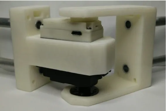
With the 3D model components tested for fitting, the STL files were exported and realised in a 3D printer. Fig.3.26a,3.26band3.26cshow a 3D rendering of the final model as well as pictures of the actual SMORA-A32 variant prototype.
24 Implementation
(a) 3D model. (b) With cover. (c) Without cover. Figure 3.26: Pictures of the final SMORA-A32 prototype.
3.1.16 BOM list
SMORA-A8 (TableA.2and TableA.3) and SMORA-A32 (TableA.4and TableA.5) have a bill of materials of under 34e in single quantities excluding PCBs and 3D printer material. Most components can be obtained through most online retailers. By procuring them directly from the manufacturer, the cost can be substantially reduced. For the development of the prototypes in this thesis, the components were either directly acquired through their manufacturer’s sample program or sourced from over-seas resellers.
3.2 Software 25
3.2
Software
Both SMORA-A8 and SMORA-A32 have a common firmware base compatible with the Ar-duino environment. This grants the open-source community an easy way to develop their own algorithms and communication protocols.
3.2.1 Bootloader
SMORA-A8 has a standard OptiBoot bootloader with a baud rate of 115200, common in most Arduino development boards. SMORA-A32 has a modified SAM-BA bootloader to use the LED as a status indicator. Both can be reprogrammed through test pads exposed in the main PCB (Fig.3.27).
Figure 3.27: SMORA-A8 ICSP.
To program the ATmega328p bootloader, a ICSP programmer is required. Open-source hard-ware designs like the USBasp are compatible. The ATSAMD21G18A however, needs to be pro-grammed through SWD (Serial Wire Debug). This can be mitigated by using, for example, a Raspberry PI Zero running the OpenOCD software.
3.2.2 Communication Protocol
To simplify the communication through the half-duplex serial interface, a protocol similar to the one incorporated in the AX-12A servo motor was written.
Communication is based on frames composed of a sequence of bytes. Each frame starts with a 5 bytes header, followed by a payload of arbitrary size and a one byte checksum. The header always starts with two OxFF bytes that allow the receiver to pinpoint the start of a new frame. Next come the identification byte, frame length byte and instruction byte. Every message ends with a checksum calculated by summing all the bytes except the first 2, taking the least significant byte and performing a NOT operation (Eq.3.1). The first byte of the payload indicates the register to where the rest of the payload is to be written.
∼ length−1
∑
n=2 byte[n] ! &0xFF (3.1)26 Implementation
Figure 3.28: Half-duplex transmitted frame at 1Mbit/s.
Fig.3.28displays the signal in the RX, TX, HalfDuplex and DIR lines, as well as the decoded bytes. The computer sets the DIR line high through the USB-to-Serial RTS pin to configure the half-duplex interface to transmission mode. The same bytes can be seen also in the TX line. The first 5 bytes contain the frame start bytes (0xFFFF), followed by ID (0x01), length (0x0B, 11 in decimal) and instruction (0x03, WRITE_REGISTER). The payloads first byte (0x02) tells the microcontroller to write 4 bytes (0x0000C842) to the GOAL_POSITION register, which is decoded as a float with the value 100, 0 in little endian. The last byte (0xE4) is the checksum obtained by Eq.3.2.
checksum=∼ (0x01 + 0x0B + 0x03 + 0x02 + 0x00 + 0x00 + 0xC8 + 0x42) & 0xFF (3.2)
Figure 3.29: Half-duplex received status frame at 1Mbit/s.
Likewise, the optional status frame in Fig.3.29shows the received bytes in the HalfDuplex and RX lines with the DIR line set low. The 5th byte (0x00) representing the instruction byte in the transmitted frame is replace with a status byte. This byte allows to diagnose failures such as checksum errors and communication faults or alarm situation such as under-voltage or over-heating. The value 0x00 indicates that there was no error. This frame is configured to echo the previously received payload so that a corruption in the transmission can be spotted.
Unlike the AX-12A, this protocol is not limited to 1 byte size registers. Having a structure that is aware of the size of each register allows the protocol to be expanded into writing to all registers forthwith from a single frame while still being able to decode their size properly.
3.2 Software 27
(a) Beginning of a frame. (b) Shortest bit.
Figure 3.30: Oscilloscope view of the half-duplex communication at 1Mbit/s.
3.2.3 Host side software
To aid in debugging, data logging and graph plotting, a host side script and library were written in Python. This script abstracts the communication layer by exposing simple commands that take care of the complexities of encoding and decoding a frame and selecting the direction of the half-duplex serial interface. The following script is sufficient to configure the position PID gains and frequency and set the desired position.
1 from smora.smora import *
2 s = Smora(port='/dev/cu.wchusbserial1420', baudrate=1000000, debug=1)
3 s.open()
4 status = s.setPIDParams(id=0x01, pid=0, Kp=0.38, Ki=0.0055, Kd=0.007, Kf=0.0,
frequency=50)
,→
5 status = s.write_data(id=0x01, register.GOAL_POSITION, 100.0)
6 s.action(id=0x01) # commit changes 7 s.close()
In order to plot the variables of interest in each test, the script uses a thread to gather the data transmitted by SMORA while the commands are being issued. When the test is complete, this data is logged to a file and plotted using the Python library matplotlib. Other mathematical functions like the Butterworth filter employed to calculate the compensator array rely on the numpy library.
3.2.4 Arduino firmware
On the firmware side, a C++ class is instantiated. This class is responsible for initialising all the microcontroller pins, sensors and interfaces and retrieving the configuration parameters (shown in the following structure) from the external EEPROM. It includes parameters such as the half-duplex identification and baud rate, PID gain parameters and the registers that can be read and written.
28 Implementation
1 typedef struct STORAGE {
2 unsigned char model = 0x02;
3 unsigned char id = 0x01;
4 unsigned long baudrate = 1000000;
5 unsigned long version = CONFIG_VERSION;
6 PID position;
7 PID speed;
8 CONTROL_T control;
9 } STORAGE;
The hot loop responsible for the core functionality of SMORA runs in the Arduino loop func-tion. By always being aware of the current time in microseconds, this loop matches the frequency to which the PID was configured, thus reducing the jitter (only minimally disturbed by interrupt routines) and making sure that values like current, voltage, temperature and present position are always retrieved periodically. It is also responsible for calculating the speed, switching between the different operation modes (position and speed control), computing the PID output, actuate on the DC motor by setting the PWM value, transmitting debugging data (if requested) and taking care of the communication.
The time required for retrieving the data from the position encoder and current, voltage and temperature sensors can be seen in Table3.1.
Table 3.1: Sensor timing
Position Current Voltage Temperature 180µs 188µs 188µs 760ms
As stated by the DS18B20 temperature sensor datasheet [17], the average time it takes for a temperature conversion is 750ms with 12-bit resolution. This of course is unacceptable if the loop function is to run at frequencies of 50Hz and above even if the temperature is only fetched once a second. To solve this issue, a non-blocking function was created that separates the start_conversion and request_temperature commands. The maximum loop time was reduced to about 6ms which allows for a PID frequency of above 150Hz.
For the communication, a state-machine function was created that is responsible for gathering the bytes sent through the half-duplex interface until their length matches the frame size, com-paring the instruction to a list of know instructions and validating the checksum. If the frame is accepted, the ID field is verified and the payload decoded and applied to the appropriate registers. In the event that a status frame is required, a payload with the reply is encoded and the bytes transmitted. Once the transmission is complete, the half-duplex direction is switched to receiv-ing mode. To prevent a deadlock in the loop, if there is a fault in the communication a timeout mechanism discards the frame and restarts the state-machine.
3.3 Algorithms 29
3.3
Algorithms
To control the motor, different algorithms were employed. They are responsible for calculating the appropriate PWM values so that SMORA can exhibit a certain desired behaviour such as setting a position or speed.
3.3.1 PID equation
The equation in2.3was discretised into3.3.
u(k) = Kpe(k) + Ki k
∑
0 e(k) F + Kd(e(k) − e(k − 1))F (3.3) where: F= PID f requency, (3.4) e= r(k) − y(k) (3.5)To prevent over-shooting from the integrator windup, an anti-windup mechanism is deployed that limits the error accumulation to a set maximum. A feed-forward loop is then combined with the PID output (3.6).
u(k) = u(k) + Kfr(k) (3.6)
The output is then scaled considering the bus voltage, constrained to the PWM allowed range and applied to it. The following code shows the compute function used to calculate the PID output.
1 float PID::compute(float ref, float error){
2 state.Reference = ref;
3 state.previous_error = state.error;
4 state.error = error;
5 state.previous_integrator = state.integrator;
6 state.integrator += state.error / pid.frequency;
7
8 // Anti-windup
9 if (state.integrator * pid.Ki > pid.limit_max){
10 state.integrator = state.previous_integrator;
11 } else if (state.integrator * pid.Ki < pid.limit_min){
12 state.integrator = state.previous_integrator;
13 }
14
15 // PID Output
16 state.Output = pid.Kp * state.error;
17 state.Output += pid.Ki * state.integrator;
18 state.Output += pid.Kd * (state.error - state.previous_error) * pid.frequency;
// same as /dt ,→
30 Implementation
19
20 // Feed-forward Output
21 state.Output += pid.Kf * state.Reference;
22 23 return state.Output; 24 } 3.3.2 Position PID Kp Ki s s Kd ∑ (s) θr ∑ -Kt ∑ 1 Js 1s b -PID Servo Drive Servo Motor Td θ(s) ω(s) G(s) Anti-windup
Figure 3.31: Diagram of the position PID.
Fig.3.31depicts the diagram for the position PID. To ensure that the shaft closely follows the position command sent by the user, the PID proportional, integral and derivative gains had to be tuned. This was accomplished by online analysis of the step-response to a variation from 100.0◦ to 110.0◦using the SMORA-A32 variant.
0 500000 1000000 1500000 2000000 us 95 100 105 110 115 de gr ee s Kp=0.5, error=3.3 Kp=0.4, Ki=0.004, error=2.12 Kp=0.365, Ki=0.003, Kd=0.006, error=0.25 Goal position
Figure 3.32: Position PID step-response with different gains.
Fig.3.32shows the step-response to different PID gains as well as the maximum position error for each one of them. With Kp=0.365, Ki=0.003 and Kd=0.006, a maximum error of 0.25◦ was
3.3 Algorithms 31
accomplished.
Tuning was achived by setting a proportional gain with zero integral and derivative. Then increasing the integral gain until the steady-state error was minimised followed by a rise in the derivative gain until there was no over-shoot. Changing one gain can affect the properties that the others try to improve. For that reason, when setting one, the others had to be slightly tweaked. By the inherent physical limitations of the system, the PID output and motor temperature were moni-tored during the tuning process to ensure that the current peaks and temperature were constrained.
0 1000000 2000000 3000000 4000000 5000000 6000000 7000000 us 60 80 100 120 140 160 180 200 220 de gr ee s Goal position Present position 0 1000000 2000000 3000000 4000000 5000000 6000000 7000000 us −250 −200 −150 −100 −500 50 100 150 200 de gr ee s/ s Present Speed 0 1000000 2000000 3000000 4000000 5000000 6000000 7000000 us −100 −80 −60 −40 −20 0 20 40 V PID Output
Figure 3.33: Position PID step-response to different position commands.
Fig.3.33shows the step-response to multiple position commands, along with the PID output in Volts and the present speed.
32 Implementation
3.3.3 Speed compensator
While testing the performance of the speed PID, a non-linear but periodic error was identified (Fig.3.34). 0 100 200 300 400 500 600 sample number 170 175 180 185 190 195 200 205 210 de gre es/ s Present speed
Figure 3.34: Present speed with a speed command of 200◦/s.
When the speed was logged over multiple rotations and ordered by angle, it became clear that the error was always similar at specific positions (Fig.3.35). The same picture shows the gathered data filtered with a 1storder Butterworth filter at the same frequency as the PID (50Hz).
0 50 100 150 200 250 300 350 400 degrees 165 170 175 180 185 190 195 200 205 210 de gr ee s/ s Present speed ButterWorth filter
3.3 Algorithms 33
This error was attributed to a misalignment in the gearbox system, as well as friction between the gears themselves. To correct for it, the concept of a Hammerstein model [24] (Fig. 3.36) was used. This model aims at improving the systems response by identifying the static nonlinear block and constructing another one that is it’s inverse function. By combining the two, the error is "canceled" and the system becomes linear dynamic.
Dynamic Linear Static
Nonlinear
u(t) x(t) y(t)
Figure 3.36: Hammerstein model.
To reduce the overhead of a lookup table for multiple speeds and positions, a single array with 360 integer values (one for each degree) was obtained from the error at a reference speed of 200.0◦/s. The value in the array index corresponding to the integer value of the present position is then subtracted from the PWM output scaled by a gain calculated from the ratio between the goal and reference speed.
Fig. 3.37shows multiple speeds with and without the compensation array applied to them. The array values can be found in TableA.1.
0
50
100
150
200
250
300
350
400
degrees
0
50
100
150
200
250
de
gre
es/
s
Present speed
Compensated speed
Figure 3.37: Plot of multiple speeds compensated.
In Fig.3.38, the symmetry in the error for the different plotted speeds at, for example, 315.0◦ reflects the gears friction at that particular position. By applying a silicon based lubricant directly to the gears, the error was slightly lessened but not eliminated.
34 Implementation
0°
45°
90°
135°
180°
225°
270°
315°
50
100
150
200
250
Present speed
Compensated speed
3.3 Algorithms 35 3.3.4 Speed PID Kp Ki s s Kd ∑ (s) ωr ∑ -Kt ∑ Js1 1s b -PID Servo Drive Servo Motor Td θ(s) ω(s) G(s) Anti-windup Kf ∑ Feed-Forward s ω(s)
Figure 3.39: Diagram of the speed PID.
Fig.3.39depicts the diagram for the speed PID. Tuning it followed the same procedure as the one used for the position PID. However, a feed-forward gain was also included.
2000000 3000000 4000000 5000000 6000000 7000000 8000000 9000000 us 100 120 140 160 180 200 de gr ee s/ s Kp=0.01, Ki=0.005, Kd=0.00022, Kf=0.0201, error=7.59 Goal speed Present speed
Figure 3.40: Speed PID step-response.
Fig. 3.40 shows the step-response to a variation in speed from 100.0◦/s to 200.0◦/s with Kp=0.01, Ki=0.005, Kd=0.00022 and Kf=0.0201. With this gains, a maximum error of 7.59◦/s was accomplished.
The speed is calculated using equation3.7.
36 Implementation
where:
F= PID f requency, (3.8)
p= position (3.9)
The function di f f Angle ensures that the angle difference is constrained between 180◦ and -180◦degrees.
1 float diffAngle(float prevAngle, float newAngle){
2 float diff = newAngle - prevAngle;
3 if (diff > 180.0) 4 diff -= 360.0; 5 if (diff < -180.0) 6 diff += 360.0; 7 return diff; 8 }
The steady-state noise in Fig.3.40and3.41can be explained by the derivative of the noise from the position sensor as the speed is being calculated in the control loop, as well as the integer and discrete nature of the speed compensator. By using an array of floats instead of integer values, this compensation can be further improved at the cost of larger overhead.
0.1 0.2 0.3 0.4 0.5 0.6 0.7 0.8 0.9 1.0 us 1e7 40 60 80 100 120 140 160 de gr ee s/ s Goal speed Present speed 0.1 0.2 0.3 0.4 0.5 0.6 0.7 0.8 0.9 1.0 us 1e7 −2 −1 0 1 2 3 4 5 V PID Output
Chapter 4
Conclusion and future work
In this last chapter, the fulfilment of the objectives for this thesis is assessed and some sugges-tions for future work are postulated.
4.1
Goal accomplishments
The objective of this thesis was to create a servo motor optimised for robotic applications. Being such a broad subject meant that the research focus had to be kept to fields like design and prototyping of 3D models and PCBs, as well as the development of the software and firmware that could perform unit tests for each of the components, control the DC motor and prove the implemented features.
At first, a literature review about servo motors and DC motor control was conducted and different techniques and approaches gathered. Research was done on similar servo motors that were designed to aid in the development of robotics.
Through reverse-engineering of an already established servo design, a 3D model was drawn to constrain the dimensions of the electronic circuit that was to ultimately replace the original one. Features present in the original enclosure like the pins that hold the potentiometer in place were repurposed to hold the PCB with the magnetic encoder circuit. After researching the current technologies used for controlling small DC motors, the final components were chosen and sourced either through the manufacturer’s sample program or other resellers.
To minimise the amount of hardware iterations and 3D printed parts until the design was finalised, the PCB was created in Eagle and modelled in 3D. This approach allowed for the overall dimensions to be verified before the PCBs and plastic parts were fabricated. The initial prototype was then manufactured by isolation routing a copper clad using a homemade CNC machine and soldering the integrated circuits. This allowed for the individual components like motor driver and current sensor to be tested and validated.
With the initial hardware verified, firmware features like controlling the shaft position started taking shape. Limitations on the bandwidth of the half-duplex circuit and the need to reposition some of the components so that the 3D enclosure would be feasible to be produced using a 3D
38 Conclusion and future work
printer led to the development of a second PCB prototype. With a PCB manufactured profession-ally, this prototype proved to be of much better quality than the first one.
Using the second prototype, additional firmware features like speed control and a proper com-munication protocol allowed for the tweaking of the PID parameters and monitoring of the motors behaviour to become swifter. With the improved software showing data that was previous unavail-able, it became apparent that there was a quality issue with the original gearbox, which led to the research of methods to mitigate it. This in turn prompt the creation of the speed compensator that substantially minimised the speed error, albeit not eliminating it completely.
The firmware was consolidated so that the position and speed control modes could be inte-grated in the same control loop as the communication protocol. A third and last iteration of the PCBs in SMORA-A8 and SMORA-A32 to correct for minor oversights was then manufactured by OSHPark.
Even though it is not included in this thesis, the initial code for a motion control algorithm with trapezoidal velocity profile was written and a SCARA robotic arm was designed and fabricated so that a proof-of-concept with two SMORA devices daisy-chained together could be accomplished. Overall, and even though the subject of the thesis was rather broad, the proposed objectives were successfully achieved with features that showed to be equivalent or even surpass the current devices available in the same price range.
4.2 Future work 39
4.2
Future work
This section describes some of the improvements that this thesis can undergo.
• Improvement of the control algorithms through parameter estimation: For the devel-opment of the proposed position and speed PIDs, the model for the motor was considered to be linear. To improve the accuracy of the control, the procedure described in the Literature Review for parameter estimation should be followed. This parameters can then be used in the feed-forward loop. Additionally, this calculations can be performed online, allowing for the control algorithms to compensate for the DC motor wear’n’tear over time or to identify the presence of different loads;
• Motion control: In order for the motion of multiple SMORA devices daisy-chained to-gether to be synchronous, a motion control algorithm based on trapezoidal velocity profile or S-curve can be incorporated [25][26]. Along with a good estimation of the DC motor parameters, this algorithms will allow for precise position and velocity control and smooth motion while minimising jerk;
• Improved gearbox: Even though the MG996R servo used in this thesis has metal gears, the original enclosure is made of plastic. Coupled with poor axis alignment, the friction in different positions burdens the PID with trying to correct for error that could be avoided. Machining a metal enclosure with the axis pins correctly aligned or choosing a different donor servo altogether could minimise this errors;
• Attitude control: Although the hardware designed for this thesis allows for the inquiry of the servos present attitude through the included MPU-6050 accelerometer and gyroscope, the firmware doesn’t take advantage of them for the control. Being a novelty in servo motor technology, this feature could be further explored so that new behaviours could be obtained. As an example, the gyroscope could be used to calibrate the 0◦ position reference for the different segments in a robotic arm. The shaft position of the servo attached to one joint could be used in conjunction with the gyroscope in the servo from the adjacent joint. By controlling the position of one while reading the data provided by the other, the whole arm can be calibrated online in a very short amount of time;
• Port hardware to other servos: The current prototypes were designed to fit into the MG996R enclosure and similar form-factor. By repositioning the components in the PCB, a generic board could be made so that other types and sizes of servos could take advantage of SMORA;
Appendix A
Figure A.1: Position encoder full schematic
42
43
44
45
(a) Top. (b) Bottom.
Figure A.5: Position encoder board.
(a) Top. (b) Bottom. Figure A.6: SMORA-A8 programmer board.
46
(a) Top.
(b) Bottom.
Figure A.7: SMORA-A8 board.
(a) Top.
(b) Bottom.
47
48
Table A.1: Speed compensation array
1-36 37-72 73-108 109-144 145-180 181-216 217-252 253-288 289-324 325-360 12 0 -3 0 2 1 -3 -3 13 -17 13 0 -3 0 2 1 -4 -2 12 -16 13 0 -3 0 1 1 -5 -1 11 -16 14 -1 -2 1 1 2 -5 0 10 -15 14 -1 -2 1 1 2 -6 0 9 -14 15 -2 -2 1 1 2 -7 2 8 -14 15 -2 -2 1 0 2 -8 3 7 -13 15 -3 -2 2 0 3 -8 4 5 -12 15 -3 -2 2 0 3 -9 4 4 -11 15 -3 -2 2 0 3 -9 5 2 -10 15 -3 -2 2 -1 3 -10 6 1 -9 15 -3 -2 2 -1 3 -10 7 0 -7 15 -3 -2 2 -2 3 -10 8 -1 -6 14 -3 -2 2 -2 3 -10 9 -3 -5 14 -3 -2 2 -3 4 -10 10 -5 -4 14 -3 -2 2 -3 4 -10 11 -6 -3 13 -3 -3 2 -4 4 -10 11 -8 -2 13 -2 -3 2 -4 4 -10 12 -9 -1 12 -2 -3 2 -4 4 -10 13 -11 0 11 -2 -3 1 -4 3 -10 14 -12 0 10 -2 -4 1 -4 3 -11 14 -13 1 10 -3 -4 1 -4 3 -10 15 -14 2 9 -3 -4 1 -4 3 -10 15 -14 2 8 -3 -4 1 -4 3 -10 16 -15 3 8 -3 -4 1 -4 3 -10 16 -16 4 7 -3 -4 1 -3 2 -10 16 -16 5 6 -3 -3 2 -3 2 -10 17 -17 5 5 -3 -3 2 -2 1 -10 17 -17 6 5 -3 -3 2 -2 1 -9 17 -17 7 4 -3 -3 2 -2 0 -9 17 -18 7 3 -3 -3 2 -1 0 -8 16 -18 8 3 -3 -2 2 -1 0 -7 16 -18 9 2 -3 -2 2 0 -1 -6 16 -18 10 1 -3 -2 2 0 -2 -5 15 -18 11 1 -3 -1 2 0 -2 -4 15 -17 11 0 -3 -1 2 0 -3 -4 14 -17 12
49
Table A.2: SMORA-A8 main PCB BOM list as of January, 2017.
Quantity Value Reference Seller Single Price Price
1 MG996R_MOTOR MG996R Aliexpress 3,52 3,52
1 DS1820 DS18B20+PAR Mouser 2,62 2,62
1 DRV8835DSSR DRV8835DSSR Mouser 1,74 1,74
1 INA219AIDCNR INA219AIDCNR Mouser 2 2
1 SN74LVC2G241DCTR SN74LVC2G241DCTR Mouser 0,651 0,651
1 ATMEGA328P_TQFP ATMEGA328P-AU Mouser 3,04 3,04
1 MIC5219 5V MIC5219-5,0YM5-TR Mouser 0,905 0,905
1 DMP3099L-7 DMP3099L-7 Mouser 0,311 0,311
1 FDN340P FDN340P Mouser 0,349 0,349
1 100F0606-RGB-CA EL-19-337/R6GHBHC-A01 Mouser 0,575 0,575
1 16MHz ABM8G-16,000MHZ-4Y-T3 Mouser 0,698 0,698
2 Molex PicoLock 504050-0491 Mouser 0,943 1,886
1 47u EMK316BBJ476ML-T Mouser 0,792 0,792
1 10u GRM188R61C106MAALD Mouser 0,321 0,321
7 100n Mouser 0,01 0,07 2 22p Mouser 0,01 0,02 1 18k CPF0402B18KE1 Mouser 0,2 0,2 1 13k CPF0402B13KE1 Mouser 0,665 0,665 6 10k AF0402JR-0710KL Mouser 0,104 0,624 1 4k7 WR04X4701FTL Mouser 0,108 0,108 1 1k WR04X1001FTL Mouser 0,108 0,108 1 0.1R RL73K3AR10 Mouser 0,124 0,124 21,327e
Table A.3: SMORA-A8 encoder PCB BOM list as of January, 2017.
Quantity Value Reference Seller Single Price Price
1 AS5048B-HTSP-500 AS5048B-HTSP-500 Mouser 6,08 6,08
1 MPU-6050 MPU-6050 Aliexpress 1,62 1,62
1 MIC5219 3,3V MIC5219-3,3YM5-TR Mouser 0,905 0,905
1 24LC16BT-I/OT 24LC16BT-I/OT Mouser 0,302 0,302
2 200mA/50V BSS138 Mouser 0,179 0,358
1 10uF GRM188R61C106MAALD Mouser 0,321 0,321
1 1u CC0402KRX5R7BB105 Mouser 0,094 0,094 4 100nF Mouser 0,01 0,04 1 10nf Mouser 0,01 0,01 1 2,2nF Mouser 0,01 0,01 1 470p VJ0402Y471KXACW1BC Mouser 0,066 0,066 5 10k AF0402JR-0710KL Mouser 0,104 0,52 10,326e
50
Table A.4: SMORA-A32 main PCB BOM list as of January, 2017.
Quantity Value Reference Seller Single Price Price
1 MG996R_MOTOR MG996R Aliexpress 3,52 3,52
1 DS1820 DS18B20+PAR Mouser 2,62 2,62
1 DRV8835DSSR DRV8835DSSR Mouser 1,74 1,74
1 INA219AIDCNR INA219AIDCNR Mouser 2 2
1 SN74LVC2G241DCUT SN74LVC2G241DCUT Mouser 0,651 0,651
1 ATSAMD21G-A ATSAMD21G18A-AU Mouser 4,58 4,58
1 MIC5219 5V MIC5219-5,0YM5-TR Mouser 0,905 0,905
1 MIC5219 3,3V MIC5219-3,3YM5-TR Mouser 0,905 0,905
1 TXB0101DBVR TXS0101DBVR Mouser 0,622 0,622
1 DMP3099L-7 DMP3099L-7 Mouser 0,311 0,311
1 FDN340P FDN340P Mouser 0,349 0,349
1 100F0606-RGB-CA EL-19-337/R6GHBHC-A01 Mouser 0,575 0,575
1 32,768KHz FX135A-327 Mouser 0,368 0,368
1 PTCSMD MF-NSMF050-2 Mouser 0,313 0,313
2 Molex PicoLock 504050-0491 Mouser 0,943 1,886
1 47u EMK316BBJ476ML-T Mouser 0,943 0,943
2 10u GRM188R61C106MAALD Mouser 0,321 0,642
3 1u GRM155R61C105KA12D Mouser 0,094 0,282 7 100n Mouser 0,01 0,07 2 22p Mouser 0,01 0,02 1 24k RG1005P-912-D-T10 Mouser 0,217 0,217 4 10k AF0402JR-0710KL Mouser 0,104 0,416 1 9.1k RG1005P-912-D-T10 Mouser 0,217 0,217 1 4k7 WR04X4701FTL Mouser 0,108 0,108 1 1k WR04X1001FTL Mouser 0,108 0,108 1 0.1R RL73K3AR10 Mouser 0,124 0,124 24.492e
Table A.5: SMORA-A32 encoder PCB BOM list as of January, 2017.
Quantity Value Reference Seller Single Price Price
1 AS5048B AS5048B-HTSP-500 Mouser 6,08 6,08
1 MPU-6050 MPU-6050 Aliexpress 1,62 1,62
1 24LC16BT-I/OT 24LC16BT-I/OT Mouser 0,302 0,302
1 10uF GRM188R61C106MAALD Mouser 0,321 0,321
1 1u CC0402KRX5R7BB105 Mouser 0,094 0,094 4 100nF Mouser 0,01 0,04 1 10nf Mouser 0,01 0,01 1 2,2nF Mouser 0,01 0,01 5 10k AF0402JR-0710KL Mouser 0,104 0,52 8.997e
References
[1] Stuart Mcfarlan (username oomlout). URL: https://www.flickr.com/photos/ snazzyguy/3465236215.
[2] Trossenrobotics. Robotis ax-12a. [Online; accessed 14 January 2017]. URL:http://www. trossenrobotics.com/dynamixel-ax-12-robot-actuator.aspx.
[3] D. Kaiser. Fundamentals of servo motion control. Motion System De-sign, 43(9):22+24+26+28, 2001. URL: https://www.scopus.com/ inward/record.uri?eid=2-s2.0-17944399301&partnerID=40&md5=
7afec604117ae23eac145a7eb3a02429.
[4] Katsuhiko Ogata. Modern Control Engineering. Prentice Hall PTR, Fourth edition, 2001. [5] J.G. Ziegler and N.B Nichols. Optimum settings for automatic controllers. Transactions of
the American Society of Mechanical Engineers (ASME), 64:759–768, 1942.
[6] M.R. Elhami and D.J. Brookfield. Identification of coulomb and viscous fric-tion in robot drives: An experimental comparison of methods. 210(6):529– 540, 1996. URL: https://www.scopus.com/inward/record.uri?eid=2-s2. 0-0030406730&partnerID=40&md5=0291f9e41f40b140dc2a7580c2df36a3. [7] J. Gonçalves, J. Lima, and P.G. Costa. Dc motors modeling resorting to a simple setup
and estimation procedure. Lecture Notes in Electrical Engineering, 321 LNEE:441– 447, 2015. URL: https://www.scopus.com/inward/record.uri?eid=2-s2. 0-84907312811&partnerID=40&md5=71134001d6fbe55c9409495c1b64dfd1, doi:10.1007/978-3-319-10380-8_42.
[8] Openservo. Openservo circuit. [Online; accessed 13 July 2016]. URL: http:// openservo.com.
[9] 01mechatronics. Supermodified servomotor. [Online; accessed 13 July 2016]. URL:http: //www.01mechatronics.com/product/supermodified-v30-rc-servos. [10] Moti. Moti servomotor. [Online; accessed 13 July 2016]. URL:http://moti.ph. [11] Robotis. Robotis ax-12a. [Online; accessed 14 January 2017]. URL: http://www.
robotis.us/ax-12a/.
[12] AMS. As5048b datasheet. [Online; accessed 20 January 2017]. URL: http://ams.com/eng/content/download/438523/1341157/file/AS5048_ DS000298_3-00.pdf.