Environmental stratification in cotton in the
presence or absence of genotypes with high
ecovalence
João Luís da Silva Filho
1*, Camilo de Lelis Morello
1, Nelson Dias
Suassuna
1, Francisco José Correia Farias
1, Fernando Mendes
Lamas
2, Murilo Barros Pedrosa
3, José Lopes Ribeiro
4and Taís
de Moraes Falleiro Suassuna
1Abstract: Cottonseed yield data of 17 genotypes, of which two genotypes con
-tributed to more than 30% of the total ecovalence, and grown in 23 locations, were used to compare four methods of disjoint environmental stratification: a) environmental index (Ie): favorable or unfavorable environments; b) stratifica -tion in parti-tions that maximize the sum of squares of the genotype x parti-tion interaction [(GP)m]; c) environmental scores of the second principal component of the GGE analysis (PC2-GGE); d) environmental scores of the first principal component of the AMMI analysis (PC1-AMMI). Scenarios were simulated (10,000 simulations per scenario) using combination of nine or 13 environ
-ments and 11 genotypes, either including or excluding those with the highest ecovalence values. In all scenarios, the greatest selection gains were obtained via PC2-GGE stratification, and the lowest selection gains were obtained via Ie. The ecovalences of the genotypes influenced the results obtained using the stratification methods.
Key words: Gossypium hirsutum, genotype x environment interaction, AMMI
and GGE biplot.
Crop Breeding and Applied Biotechnology
17: 32-39, 2017
Brazilian Society of Plant Breeding. Printed in Brazil http://dx.doi.org/10.1590/1984-70332017v17n1a5
ARTICLE
*Corresponding author: E-mail: [email protected]
Received: 24 November 2015 Accepted: 09 June 2016
1 Embrapa Algodão, CP 147, 58.428-095,
Campina Grande, PB, Brazil
2 Embrapa Agropecuária Oeste, CP 661,
79.804-970, Dourados, MS, Brazil
3 Fundação Bahia, Rodovia BR 020/242,
S/N, km 50,7, 47.850-000, Zona Rural, Luís Eduardo Magalhães, BA, Brazil
4 Embrapa Meio-Norte, CP 01, 64.006-220,
Teresina, PI, Brazil
INTRODUCTION
The development and release of cotton cultivars in Brazil follows growers’ demands for competitive lint yield, and fulfill industrial textile requirements, in particular in the Cerrado environment, the largest cotton growing area in Brazil (Morello et al. 2010, Morello et al. 2012, Morello et al. 2015). Prior to cultivars being recommended, multiple trials (different locations and/or growing seasons) are carried out to evaluate genotypes in different growing conditions. However, in general, the performance of genotypes across environments may not be consistent, due to the genotype x environment interaction (GEI).
In regression models, the genotype performance is adjusted in function of the environmental index (Ie), categorized
as unfavorable or favorable, according to their respective performance related to the overall means. It is assumed that selection gains are higher when cultivar recommendation assigns them to one of these categories. The models of Toler and Burrows (1998) and AMMI may be used simultaneously to study and estimate the effects of phenotypic stability (Ferreira et al. 2006).
On the other hand, for AMMI and GGE, PC analysis is carried out to capture patterns of the GEI and make inferences from graphic dispersion. The difference between models is the data matrix used. AMMI is a double centered PC analysis and GGE is environment-centered PC analysis (Gauch et al. 2008). Considerations and comparisons of both methods are found in the literature (Gauch 2006, Yan et al. 2007, Gauch et al. 2008, Yang et al. 2009, Balestre et al. 2009, Oliveira et al. 2010).
Although the mathematical and statistical properties of the models used in the GEI studies are well established, it is important to know how genotypes and environments affect the interaction (Crossa et al. 2015). The ecovalence is a relative contribution of each genotype for the GEI and a measure of the agronomic stability. The genotypes that follow the mean environment performance are considered more stable (Ramalho et al. 1993). The smaller the estimated ecovalance, the more stable is the genotype.
However, there is lack of information about the influence of genotype ecovalence on the efficiency of stratification methods. In a simulation study, Ferraudo and Perecin (2014) concluded that the AMMI and Eberhart and Russel models, and mixed models, in addition of detecting different aspects of GEI, detected the interactions only for the genotypes with considerable ranking exchanges across environments. Furthermore, although the methods based on multivariate analysis are widely used to discard environments, there is little information on whether such methods are influenced by the number of genotypes and of environments.
This study aimed at comparing four models of environmental stratification, simulating the presence or absence of high ecovalence genotypes, when the number of environments is higher or lower than the number of genotypes.
MATERIAL AND METHODS
Experimental data
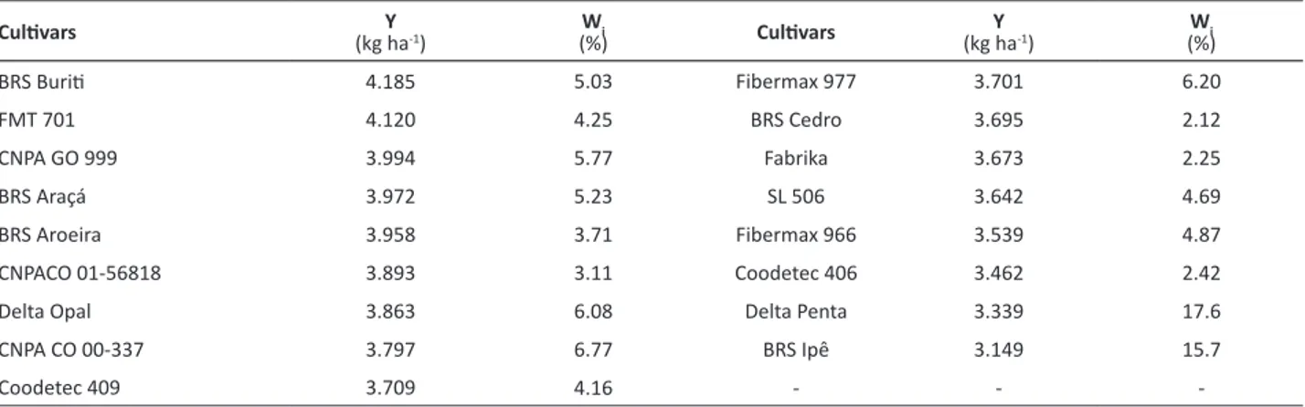
Cottonseed yield data obtained from 17 cotton cultivars evaluated in 23 locations in the Brazilian Cerrado were used in this study (Silva Filho et al. 2008). The ecovalence of two cultivars, BRS Ipê and Delta Penta, hereinafter referred to as high ecovalence cultivars (HEC), contributed for more than 30% of the sum of squares of the GEI (Table 1). This information is relevant for the understanding of the methodology described below.
Stratification methods
Using a process of resampling of the original data, four methods of environmental stratification and a control with no stratification were compared. Disjoint classifications in two groups were used to facilitate the implementation of the routines and the categorization of environments in one of the groups. If the study aimed at grouping the environments into macro-regions, it is probable that grouping in more than two strata would be necessary. In each resampling (simulation), the following methods were applied:
i) control (no environmental stratification): equivalent to selecting the genotype with the best mean performance across environments;
ii) stratification by environmental index (Ie): locations with yield above the overall mean constituted a group (favorable
environment), and locations below the overall mean constituted the other group (unfavorable environment);
iii) stratification by maximization of the sum of squares of genotype x partition - (GP)m: the sum of squares of the
GEI can be decomposed into SSGEI = SSGEI1(P1) + SSGEI2(P2) + SSGP, in which SSGEI1(P1) is the sum of the squares of the
GEI within partition 1; SSGEI2(P2) is the sum of squares of the GEI within partition 2; and SSGP is the sum of squares
environments is C
n,1 + Cn,2 + ... + Cn,n/2 taking the whole part to the decimal “n/2” values. This method was used only
as a maximization reference of the interaction between the two groups, since it is impractical when a high number of environments is evaluated.
iv) stratification by environment PC2 scores of the GGE analysis (PC2-GGE): according to Yan and Hunt (2001), scores of the first PC of the GGE analysis are associated with the simple part of the GEI, while the scores of the second PC are associated with the crossover GEI. Thus, the environment PC2 scores were adopted as reference, considering the environments with negative score in a group, and those with positive scores in another group.
v) stratification by environment PC1 scores of the AMMI analysis (AMMI): Gauch et al. (2008) reported that PC1-AMMI and PC2-GGE are highly correlated. Thus, the environment PC1 scores were used considering the environments with negative score in a group, and those with positive scores in another group.
Scenarios in which the methods were compared
The highest number of possible combinations of n elements taken k at a time, Cn,k, occurs if k is equal to n/2 (or near the whole number). In this case, with 23 environments, k = 11 or 12; for 17 genotypes, k = 8 or 9. We assume that the higher the values of Cn,k, the higher are the chances of representing different situations of the GEI. Considering that one of the goals was to evaluate scenarios with higher or lower number of environments than the number of genotypes, nine or 13 environments and 11 genotypes, which included or not the HEC, were resampled. Therefore, the four methods and the control were compared in four scenarios:
i) number of environments lower than the number of genotypes, with the presence of HEC - 10,000 simulations by resampling of the original matrix (17 genotypes x 23 environments), considering nine environments and 11 genotypes. In this case, in each resampling, nine environments were randomly sampled among the 23; the two HEC (BRS Ipê and Delta Penta) were always present, and the other nine genotypes were randomly selected among the remaining 15.
ii) number of environments lower than the number of genotypes, without the presence of HEC - 10,000 simulations by resampling of the original matrix, considering nine environments and 11 genotypes. Similarly to the previous scenario, nine environments were randomly selected among the 23; the two HEC were excluded from the resampling process. The 11 genotypes were randomly sampled among the remaining 15.
iii) number of environments higher than the number of genotypes, with the presence of HEC - 10,000 simulations considering 11 genotypes and 13 environments randomly sampled among the 23 environments. The two HEC were always present, and the other nine genotypes were sampled among the remaining 15;
iv) number of environments higher than the number of genotypes, without the presence of HEC - 10,000 simulations considering 11 genotypes and 13 environments randomly selected among the 23 environments, and 11 genotypes selected among 15, excluding the two HEC.
Regarding the stratification method (iii), (GP)m, in each one of the 10,000 simulations per scenario, all the 255 or
4095 stratification possibilities (nine or 13 environments, respectively) were included. Thus, for the latter situation, more than 40 million tests per scenario were computed.
Criteria for comparison between the stratification methods
At the end of the 10,000 simulations in each scenario, the following criteria were calculated for each method: i) mean selection gains (SG): in each simulation, for each group, the genotype with the highest cottonseed yield was assumed to be the best genotype. Then, the weighted mean of the best genotypes was calculated with the number of environments as weight. The SG (as a percentage) was calculated by the difference between the weighted mean and the overall mean of the sample, divided by the overall mean of the sample. The mean values of these percentages in 10,000 simulations were then calculated for each stratification method. For the control method, this criterion corresponds to selecting the genotypes with the best mean performance in the sample.
each simulation, taking the mean value of the simulations for each stratification method. The values of this criterion for the method (iii), (GP)m, are reference values, since, they are the mean of the maximum values for this statistic obtained
in the simulations.
iii) percentage of wins (PW): number of simulations where the stratification method have the highest SG value, in the 10,000 simulations for each scenario;
iv) percentage of exclusive wins (PEW): number of simulations where the stratification method had exclusively the highest SG value, in the 10,000 simulations for each scenario;
v) percentage of common wins between the pairs of methods (PCW): number of simulations where each pair of stratification methods had the highest GS value, in 10,000 simulations for each scenario;
vi) Pearson’s correlation between the GS and the GP: Pearson’s correlation was calculated between SG and GP, for each method, in each scenario, considering the 10,000 simulations.
All analyses were carried out in the R environment, including the routines for each one of the stratification method. All routines were based on functions and commands previously available in R (“sample”, “colMeans”, “rowMeans”, “SVD”, among others).
RESULTS AND DISCUSSION
Table 1 shows the mean cottonseed yield and ecovalences estimates for 17 cotton cultivars evaluated in 23 locations. The two cultivars with the lowest yield, BRS Ipê and Delta Penta, contributed with more than 30% to the GEI, and according to Silva Filho et al. (2008), they are not well adapted to any of the 23 locations evaluated.
In such situations, one may question whether the presence of genotypes with high ecovalence can influence the stratification patterns given by AMMI or GGE analysis either on the magnitude of the GEI captured by the eigenvalues, or on the dispersion graphic.
Table 2 shows the mean values of the comparison criteria for the stratification methods in different scenarios simulated. As expected, the SG values in the absence of environmental stratification (control) were the lowest in all scenarios, since, at worst, the best genotype of a group should be the best genotype in the overall mean whatever the partitioning of the groups of environment may be. Thus, there is no PEW for the control method, and PW indicates the percentage of simulations in which all the methods simultaneously provided the same SG. The simultaneous agreement ranged from 4.5 to 7.8%, being higher, in absolute terms, in the presence of the HEC and, or, in more environments. According to the results, the more complex the GEI, the more similar to each other the methods tend to be, possibly due to greater difficulty in identifying patterns.
Table 1. Mean cottonseed yield (Y) and ecovalences estimates in percentage (W
i) for 17 cotton cultivars evaluated in 23 locations of
the Brazilian Cerrado
Cultivars Y
(kg ha-1)
Wi
(%) Cultivars (kg haY -1)
Wi
(%)
BRS Buriti 4.185 5.03 Fibermax 977 3.701 6.20
FMT 701 4.120 4.25 BRS Cedro 3.695 2.12
CNPA GO 999 3.994 5.77 Fabrika 3.673 2.25
BRS Araçá 3.972 5.23 SL 506 3.642 4.69
BRS Aroeira 3.958 3.71 Fibermax 966 3.539 4.87
CNPACO 01-56818 3.893 3.11 Coodetec 406 3.462 2.42
Delta Opal 3.863 6.08 Delta Penta 3.339 17.6
CNPA CO 00-337 3.797 6.77 BRS Ipê 3.149 15.7
Coodetec 409 3.709 4.16 - -
It should be noted that identical SG values do not necessarily imply that the methods identified identical partitions, since the same genotype could be the winner in the partitions obtained by each method, or different partitions with different genotypes selected could provide identical SG value. In all scenarios, the descending order of PW and SG was: PC2-GGE, PC1-AMMI, (GP)m, and Ie. Therefore, discussion was organized by comparing a given stratification method
with the one immediately superior in performance.
Comparing Ie and (GP)m is the same as comparing a strategy based on scale effect, Ie, and another that maximizes the
variance of the interaction between groups, (GP)m. In all scenarios, the GP values captured by the method (GP)m were
almost three times the value of Ie, and PW of (GP)m were always higher than those of Ie (Table 2). In situations in which
HEC were present, the PEW obtained in Ie were higher.
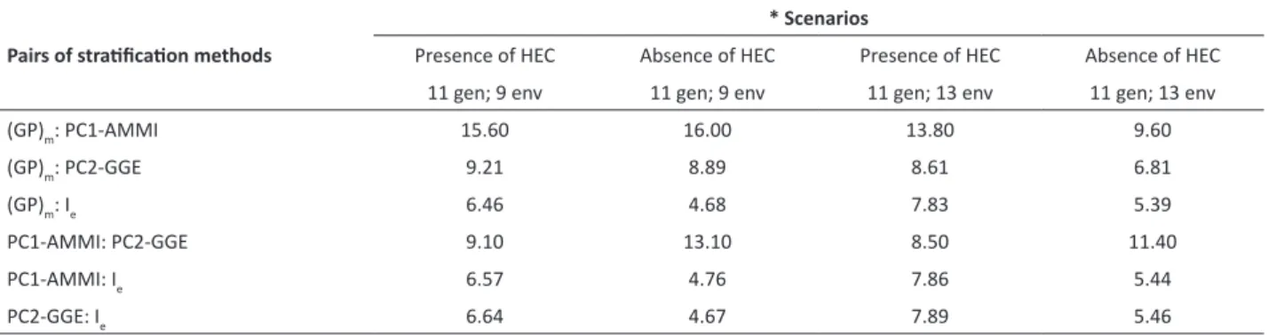
The Ie was the method that correlated less with the others, since PCW were very close to the PW of the control
(Table 3). For instance, in the presence of HEC with 11 genotypes and nine environments, PCW between (GP)m and
Ie was 6.5%, while the PW of the control was 6.4%. This may due to the fact that Ie does not use variance in the
stratification process.
Despite retaining little of the GEI between partitions, the Ie method was the only one with negative Pearson’s
correlations between SG and GP, with higher values, in modulus, in the absence of HEC (Table 2).
Table 2. Mean percentage values of selection gains (SG), ratio of sum of squares of the genotype x partitions interaction and the sum
of the squares of the total interaction (GP), percentage of wins (PW), percentage of exclusive wins (PEW), and Pearson’s correlation (r) between SG and GP, obtained for two sample sizes, in the presence or absence of high ecovalence cultivars (HEC), for each of the stratification methods
Sample size
Stratification method Presence of HEC Absence of HEC GP
(%) (%)SG PW(%) PEW(%) r (%)GP (%)SG PW(%) PEW(%) r
(GP)m 47.2 13.2 25.0 7.5 0.06 34.7 11.4 30.7 12.8 0.05
11 genotypes PC1-AMMI 42.6 13.5 29.9 12.5 0.12 31.1 11.6 41.2 19.0 0.16
9 enviroments PC2-GGE 23.8 14.1 57.8 46.7 0.12 23.7 11.7 49.0 34.0 0.27
Ie 16.7 13.1 20.6 13.8 -0.03 13.6 10.6 15.1 10.1 -0.13
*Control - 12.2 6.4 - - - 9.7 4.5 -
-(GP)m 42.8 12.5 23.7 9.4 0.03 28.4 10.6 28.8 18.4 0.06
11 genotypes PC1-AMMI 38.3 12.6 26.1 11.8 0.13 25.1 10.7 33.9 18.9 0.11
13 environments PC2-GGE 18.6 13.3 63.3 54.2 0.12 19.5 11.0 52.3 40.0 0.26
Ie 13.3 12.3 17.6 9.7 -0.04 9.4 9.8 12.3 6.8 -0.18
*Control - 11.8 7.8 - - 9.3 5.4 -
-* No stratification
Table 3. Percentage of common wins between the pairs of methods, in different simulated scenarios
Pairs of stratification methods
* Scenarios
Presence of HEC Absence of HEC Presence of HEC Absence of HEC 11 gen; 9 env 11 gen; 9 env 11 gen; 13 env 11 gen; 13 env
(GP)m: PC1-AMMI 15.60 16.00 13.80 9.60
(GP)m: PC2-GGE 9.21 8.89 8.61 6.81
(GP)m: Ie 6.46 4.68 7.83 5.39
PC1-AMMI: PC2-GGE 9.10 13.10 8.50 11.40
PC1-AMMI: Ie 6.57 4.76 7.86 5.44
PC2-GGE: Ie 6.64 4.67 7.89 5.46
The results of the present study do not support the widely diffused recommendation of cultivars based on defining favorable or unfavorable environments. However, it should be noted that the PEW obtained in the different scenarios (from 6.8 to 13.8%) shows that, in some situations, the more complex models were not efficient to evaluate SG.
Although (GP)m was slightly superior to Ie, showing advantage in incorporating variance information on environmental
stratification, maximizing GP was not efficient when the objective was to increase SG, since Pearson’s correlations between SG and GP were very low, ranging from 0.03 to 0.06 (Table 2). Even if this method was advantageous in relation to the others, the computational cost to try all possible environments partitions into two groups would make it impractical in situations with high numbers of environments; therefore, it should be interpreted as a reference in relation to the capture of the GP.
In all scenarios, the PC1-AMMI method had higher SG, PW, and PEW than (GP)m. Results confirm the classic assumption
conferred to the AMMI analysis, which is able to separate the variation of interaction into pattern and noise, and it is not appropriate to completely explore the GEI, at least for partitions disjoined into two groups.
PC1-AMMI and (GP)m had the greatest PCW between each other in three of the four scenarios (Table 3), always
superior to 9.5%. Taking the ratio between PCW of the two methods and the PW of (GP)m, a measure of how PC1-AMMI
could be used in substitution of (GP)m was obtained. In this regard, the best scenario is that where the number of
environments is lower than that of genotypes, and where HEC are present: 62.4% (15.6 ÷ 25.0); and the worst scenario, 33.3% (9.6 ÷ 28.8), is when the number of environments is superior to that of genotypes, and HEC are absent. Thus, it is useful to consider whether, and how, more complex AMMI models would be able to identify the partitions in which (GP)m was superior to PC1-AMMI.
On the other hand, our results did not corroborate some of the consolidated and well disseminated statements regarding the use of AMMI analysis. In the evaluation of an AMMI model, besides the number of PCs to be chosen, a primary consideration is how much of the variation is explained by the first PC capture (Lavoranti et al. 2007, Yang et al. 2009, Gauch 2013). There were higher values for GP when HEC was present, while higher PW and PEW were observed in the absence of HEC. Indeed, scenarios with higher captures of the GEI via GP were not those in which PC1-AMMI had better evaluations when compared with the others (Table 2). Pearson’s correlations between SG and GP obtained for the PC1-AMMI method was low (< 0.16), but higher than those for (GP)m.
The presence of HEC may have influenced the pattern and magnitude of the GEI captured in the first PC of the AMMI analysis. With GEI concentrated in a few genotypes, decomposition via SVD (singular values decomposition) seems to
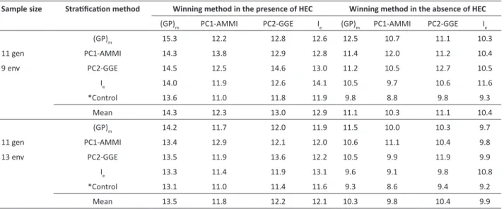
Table 4. Selection gains (%) obtained by each stratification method in simulations that a given method was exclusive winner in the
different scenarios simulated (two sample sizes, in the presence or absence of high ecovalence cultivars - HEC)
Sample size Stratification method Winning method in the presence of HEC Winning method in the absence of HEC
(GP)m PC1-AMMI PC2-GGE Ie (GP)m PC1-AMMI PC2-GGE Ie
(GP)m 15.3 12.2 12.8 12.6 12.5 10.7 11.1 10.3
11 gen PC1-AMMI 14.3 13.8 12.9 12.8 11.4 12.0 11.2 10.4
9 env PC2-GGE 14.5 12.5 14.6 13.0 11.2 10.5 12.7 10.5
Ie 14.0 11.9 12.6 14.1 10.5 9.7 10.6 11.6
*Control 13.6 11.0 11.8 11.9 9.8 8.8 9.8 9.3
Mean 14.3 12.3 13.0 12.9 11.1 10.3 11.1 10.4
(GP)m 14.2 11.7 12.0 11.9 11.5 10.0 10.3 9.7
11 gen PC1-AMMI 13.4 12.9 12.1 12.0 10.6 11.1 10.4 9.8
13 env PC2-GGE 13.5 11.9 13.6 12.2 10.5 9.9 11.9 9.9
Ie 13.3 11.4 11.9 13.1 9.6 9.1 9.8 10.8
*Control 13.1 11.0 11.4 11.6 9.3 8.6 9.4 9.2
Mean 13.5 11.8 12.2 12.1 10.3 9.8 10.4 9.9
seek this pattern. In the study of Silva Filho et al. (2008), the two HEC presented, in modulus, the highest scores of the first PC. These considerations are supported by Ferraudo and Perecin (2014), who claim that the AMMI model is efficient to capture interaction when there is strong fluctuation in the ranking of genotypes along the environment, i.e., with high ecovalence.
In all scenarios, when comparing PC2-GGE and PC1-AMMI, the estimates of SG, PW and PEW were higher in PC2-GGE, while those of GP were higher in PC1-AMMI. An explanation for GP values is that, in SVD analyzes, the first PC always captures more variation than the second, although the data matrices used by PC1-AMMI and PC2-GGE are different. Including the genotype´s effects in the GGE analysis may lead to a buffering effect to the estimates of GP, since there was little variation in the presence or absence of HEC for the same scenario of sample size (Table 2).
Gauch et al. (2008) stated that the PC1 of the AMMI analysis is highly correlated with the PC2 of the GGE analysis. However, the PCW values between the two methods were slightly lower than 10% in the presence of HEC, and slightly greater than this value in the absence of HEC (Table 3). The ratio between the PCW values of the two methods and PW values of the PC1-AMMI is an estimate on how close PC2-GGE is from PC1-AMMI. When including HEC, these values were 30.4% (9.1 ÷ 29.9), when 11 genotypes and nine environments were analyzed, and 32.6% (8.5 ÷ 26.1), when 11 genotypes and 13 environments were simulated. In the absence of HEC, these values were 31.8% (13.1 ÷ 41.2) and 33.6% (11.4 ÷ 33.9), respectively.
The combined use of AMMI and regression models to address different aspects of GEI has been reported (Ferreira et al. 2006, Ferraudo and Perecin 2014). This approach supports that stratification-PC2 via GGE as the most satisfactory method. Indeed, Yan et al. (2007) stated that the original model of the GGE analysis is also called regression model sites or locations (SREG - linear-bilinear regression model site), a multivariate regression.
However, results do not allow the exclusive recommendation of PC2-GGE. In the scenario with the highest PW and PEW for this method (with 11 genotypes, 13 environments and including HEC), there was 63.3% PW, and 54.2% PWE. Thus, in approximately 36% of the cases, there are potentially more efficient models regarding cultivars recommendation. Furthermore, PC1-AMMI and/or PC2-GGE identified the greatest SG of 74.8 to 80.9% (PWPC1-AMMI + PWPC2-GGE – PCW
PC1-AMMI:PC2-GGE). Thus, in at least 20% of the cases, the partitions that provided greater SG were not identified by these methods.
The PC2-GGE method presented its lower estimates of PW and PEW in scenarios where HEC were excluded from the simulations. In the data set used, HEC were among the low yielding cotton cultivars. The inclusion or exclusion of HEC may have changed the magnitude of GEI in the samples. However, these considerations may not be extended in cases where the HEC are among the high yielding, a matter of great practical concern. Unfortunately, no data set with such configuration was available. Thus, choosing the stratification methods goes beyond measuring, decomposing, and capturing the GEI in the partitions found by a particular method. It is important to know the nature of the GEI, how it is affected by genotypes and whether specific levels of treatments are decisive for the interaction, as mentioned by Crossa et al. (2015).
In order to verify if the stratification methods explore different aspects of GEI, we computed the SG, for each method, when a given method was exclusive winner (Table 4). When PC1-AMMI was exclusive winner, in general, smaller SG were obtained for all methods; on the other hand, when (GP)m was exclusive winner, higher SG were observed. Increasing the
number of environments reduces the SG by any method. The SG in the presence and absence of HEC are not comparable, since the simulations were carried out on the data set with different means.
Specific levels of treatment, such as genotypes of high ecovalence, can be decisive in the study of the GEI, influencing the choice of the stratification method. The Ie method is the least recommended for a general use, and it presents
less correlation with the other methods. While bearing in mind that there are situations in which other methods are potentially more advantageous, we believe that stratification by PC2-GGE should be recommended.
ACKNOWLEDGEMENTS
REFERENCES
Balestre M, Pinho RG, Souza J C and Oliveira RL (2009) Genotypic stability and adaptability in tropical maize based on AMMI and GGE biplot
analysis. Genetics and Molecular Research8: 1311-1322.
Crossa J, Vargas M, Cossani CM, Alvarado G, Burgueño J, Mathews KL and Reynolds MP (2015) Evaluation and interpretation of interactions.
Agronomy Journal107: 736-747.
Eberhart SA and Russell WA (1966) Stability parameters for comparing varieties. Crop Science 6: 36-40.
Ferraudo GM and Perecin D (2014) Mixed model, AMMI and Eberhart-Russell comparison via simulation on genotype × environment
interaction study in sugarcane. Applied Mathematics 5: 2107-2119.
Ferreira DF, Demétrio CGB, Manly BFJ, Machado AA and Vencovsky R (2006) Statistical models in agriculture: biometrical methods for evaluating phenotypic stability in plant breeding. Cerne12: 373-388.
Gauch HG (2006) Statistical analysis of yield trials by AMMI and GGE.
Crop Science 46: 1488-1500.
Gauch HG (2013) A simple protocol for AMMI analysis of yield trials. Crop
Science 53: 1860-1869.
Gauch HG and Zobel RW (1996) AMMI analysis of yield trials. In Kang
MS and Gauch HG (ed) Genotype by environment interaction. CRC
Press, New York, p. 85-122.
Gauch HG, Piepho HP and Annicchiarico P (2008) Statistical analysis of
yield trials by AMMI and GGE: further considerations. Crop Science
48: 866-889.
Lavoranti OJ, Dias CTS and Kraznowski WJ (2007) Phenotypic stability
via AMMI model with Bootstrap re-sampling. Boletim de Pesquisa
Florestal 2: 45-52.
Morello CL, Pedrosa MB, Suassuna ND, Lamas FM, Chitarra LG, Silva JL, Andrade FP, Barroso PAV, Ribeiro JL, Godinho VPC and Lanza MA (2012) BRS 336: a high-quality fiber upland cotton cultivar for Brazilian
savanna and semi-arid conditions. Crop Breeding and Applied
Biotechnology 12: 92-95.
Morello CL, Suassuna ND, Barroso PAV, Silva Filho JL, Ferreira ACB, Lamas
FM, Pedrosa MB, Chitarra LG, Ribeiro JL, Godinho VPC and Lanza MA (2015) BRS 369RF and BRS 370RF: Glyphosate tolerant, high-yielding
upland cotton cultivars for central Brazilian savanna. Crop Breeding
and Applied Biotechnology 15: 290-294.
Morello CL, Suassuna ND, Farias FJC, Lamas FM, Pedrosa MB, Ribeiro JL, Godinho VPC and Freire EC (2010) BRS 293: A midseason
high-yielding upland cotton cultivar for Brazilian savanna. Crop Breeding
and Applied Biotechnology 10: 180-182.
Oliveira RL, Pinho RG, Balestre M and Ferreira DV (2010) Evaluation of maize hybrids and environmental stratification by the methods
AMMI and GGE biplot. Crop Breeding and Applied Biotechnology
10: 247-253.
Ramalho MAP, Santos JB and Zimmermann MJO (1993) Genética
quantitativa em plantas autógamas: aplicações ao melhoramento
do feijoeiro. UFG, Goiânia, 271p.
Silva Filho JL, Morello CL, Farias FJC, Lamas FML, Pedrosa MB and Ribeiro JL (2008) Comparação de métodos para avaliar a adaptabilidade
e estabilidade produtiva em algodoeiro. Pesquisa Agropecuária
Brasileira 43: 349-355.
Toler JE and Burrows PM (1998) Genotype performance over environment arrays: a non-linear grouping protocol. Journal of Applied Statistics 25: 131-143.
Yan W and Hunt LA (2001) Interpretation of genotype x environment interaction for winter wheat yield in Ontario. Crop Science 41: 19-25.
Yan W, Fetch JM, Frégeau-Reid J, Rossnagel B and Ames N (2011) Genotype x locations interactions patterns and testing strategies for oat in
Canadian prairies. Crop Science 51: 1903-1914.
Yan W, Hunt LA, Sheng Q and Szlavnics Z (2000) Cultivar evaluation and
mega-environment investigation based on the GGE biplot. Crop
Science 40: 597-605
Yan W, Kang MS, Ma B, Woods S and Cornelius PL (2007) GGE biplot vs.
AMMI analysis of genotype-by-environment data. Crop Science 47:
643-653.
Yang RC, Crossa J, Cornelius PL and Burgueño J (2009) Biplot analysis
of genotype environment interaction: Proceed with caution. Crop