Evaluation of maize hybrids and environmental stratification by the methods AMMI and GGE biplot

(1)

Crop Breeding and Applied Biotechnology 10: 247-253, 2010 Brazilian Society of Plant Breeding. Printed in Brazil

Received 18 December 2009

Accepted 12 May 2010

Evaluation of maize hybrids and environmental

stratification by the methods AMMI and GGE biplot

Rogério Lunezzo de Oliveira1* Renzo Garcia Von Pinho2, Márcio Balestre1, and Denys Vitor Ferreira3

ABSTRACT -The purpose of this study was to evaluate yield stability, adaptability and environmental stratification by the methods AMMI (Additive Main Effects and Multiplicative Interaction Analysis) and GGE (Genotype and Genotypes by Environment Interaction) biplot and to compare the efficiency of these methods. Data from the evaluation of 20 experimental single-cross and three commercial hybrids and 11 locations, in two growing seasons, 2005/2006 and 2006/2007 were used. Analyses of variance, adaptability, stability and environmental stratification were performed. A better combination of adaptability and stability was observed in the hybrids 10 and 16, according to the graphics of AMMI and GGE biplot methods, respectively. The number of locations could be reduced by 28% based on stratification. The predictive correlation of the AMMI and GGE methods was 0.88 and 0.86, respectively. The results showed that it is possible to reduce the number of evaluation sites; AMMI tended to be more accurate than GGE analysis.

Key words: Zea mays, genotype by environment interaction, mega-environments.

INTRODUCTION

The genotype by environment interaction (GE) may be reduced using specific cultivars for each environment or using cultivars with wide adaptability and good stability or by stratifying the region under study in mega-environments with similar environmental characteristics, within which the interaction becomes insignificant (Terasawa Júnior et al. 2008).

There are several methodologies to assess the GE, of which the most commonly used are based on simple and multiple regression. Despite the widespread use, regression-based methods have limitations that are frequently reported in the literature. Crossa (1990) argues that linear regression analysis is not informative if linearity

fails, is highly dependent on the group of genotypes and environments included, and tends to simplify response models explaining the variation caused by interaction in one dimension, when in fact it can be quite complex.

Crossa (1990) suggested that the application of multivariate methods can be useful to better exploit the information contained in the data. He proposed techniques such as principal component analysis (PCA), cluster analysis and the AMMI procedure (Additive Main Effects and Multiplicative Interaction Analysis), which have gained wide application in recent years. A detailed description of the AMMI methodology is given by Ebdon and Gauch (2002) and Duarte and Vencovsky (1999). The AMMI model has also been used for environmental stratification, and stratification based on the winning

1 _{Universidade Federal de Lavras (UFLA), Departamento de Biologia, C.P. 3037, Lavras, MG, Brazil. E-mail: rlunezzo@yahoo.com.br.} 2

UFLA, Departamento de Agricultura.

(2)

genotypes has been more efficient than of other stratification methods (Pacheco et al. 2003).

Recently, a modification of conventional AMMI analysis, proposed by Yan et al. (2000), denoted GGE (Genotype and Genotype-by-Environment Interaction) biplot, has been used to study the genotype by environment interaction. GGE analysis groups the genotype effect, which is an additive effect in the AMMI analysis, with the GE interaction, which is a multiplicative effect, and subjects these effects to a multiplicative model for local regression (SREG - Site Regression).

The purpose of this study was to evaluate yield stability, adaptability and environmental stratification by the methods AMMI and GGE biplot, using test data to evaluate maize hybrids and compare the efficiency of the methods.

MATERIAL AND METHODS

Grain yield data of the final trials of maize hybrids were used, provided by the company Monsanto. The tests were performed in a randomized block design (three replications in the 2005/2006 and two replications in the 2006/2007 growing season) at 11 locations in two growing seasons, in a total of 22 environments, in the states Minas Gerais, São Paulo, Paraná, Goiás, Mato Grosso do Sul, Bahia and Distrito Federal (Table 1). The plots consisted of four 5-m rows and the evaluated area per plot was 7.5 m2_{. Of the 23 evaluated hybrids, 20 were experimental and}

three commercial hybrids (described in Table 1).

To assess the genetic variability among the treatments (hybrids) and the experimental accuracy, analysis of variance was performed for each environment (individual analysis). Then a combined analysis was carried out, as proposed by Ramalho et al. (2000), considering the genotype and environment effects as fixed. For the analyses of variance

proc glm was used, of the software package SAS v 8.0 (SAS Institute 2000).

Once the presence of GE interaction (F test significant) was confirmed, the stability analysis was carried out, which allows a measurement of adaptabilityand yield stability of each test hybrid. The AMMI and GGE biplot were used in the assessment in order to compare the efficiency of these methods. The AMMI analysis was performed using the software Estabilidade, developed by Ferreira and Zambalde (1997), while the GGE biplot analysis was performed using SAS v 8.0, with IML (Interactive Matrix Language) and SAS GRAPH (SAS Institute 2000).

The AMMI analysis according to Zobel et al. (1988) combines in a single model additive components for the main effects of genotype (gi) and environments (ej), and

multiplicative components for the effect of GE interaction (geij). The model that describes the mean yield of a genotype

i in environment j is given by: Yij = µ + gi + aj + Σ λkγikαjk +

rij + εijwhere: Yij is the average yield of genotype i in environment j, Yij is the overall mean yield; gi is the effect of genotype I; aj is the effect of environment j; λk is the k-th singular value of the original matrix interactions (GE); γik is the element corresponding to the i-th_{genotype in the}_k-th singular vector of the GE matrix column; αjk is the element corresponding to the j-th_{environment in the}_k-th_singular vector of the GE matrix row; rij is the noise associated with the expression (geij) not explained by the retained principal components; n is the number of axes or principal components retained to describe the GE interaction pattern;

εij is the average experimental error associated with observation, assumed to be independent ε ~N(0, σ2₎_.

For the GE interaction, the biplot is interpreted by observing the magnitude and sign of the scores of genotypes and environments, for the axis (axes) of interaction. Thus, low scores (close to zero) represent genotypes and environments are little involved in the interaction and are characterized as stable. In an AMMI2 biplot, the points of stable genotypes and environments

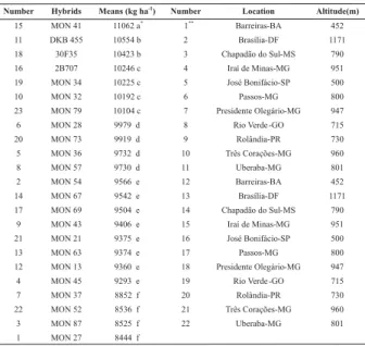
Table 1. Identification of 23 hybrids, with their respective mean yield, and of 22 environments

* Means followed by the same letter did not differ from each other by the Scott-Knott test at 5% probability.

** ** ** **

** Number 1 to 11 (growing season 2005/2006), number 12 to 22 (growing season 2006/2007).

(3)

(with little contribution to the sum of squares of the GE interaction (SSGE)) lie near the origin.

To stratify the environments, the methodology AMMI was used with the approach of winning genotypes, as proposed by Gauch and Zobel (1997). In this study, the groups were obtained by estimates of the interaction of AMMI1. Thus, the strata were defined by the winning genotype. In this context, each genotype with one or more winning genotypes, i.e., the genotype with the highest mean yield in one or more environments, determines an environmental stratum.

To verify the efficiency of SREG, denoted GGE biplot (Genotype and Genotype-by-Environment Interaction), by Yan et al. (2000), in explaining the effect of genotypes (G) + (GE) interaction in relation to the AMMI analysis, the GGE analysis was performed, using SAS v. 8.0 (SAS Institute 2000) considering the simplified model for two principal components: Yij - µj = λ1γi1αj1+λ2γi2αj2 + ρij + εij, where Yij is the mean yield of cultivar i in environment j; µj is the mean of environment j; λ1γi1αj1 is the first principal component (PCA1); λ2γi2αj2 is the second major component (PCA2); λ1 and λ2 are the eigenvalues associated to PCA1 and PCA2; γi1 and γi2 are the scores of PCA1 and of PCA2, respectively, for the genotype effect;

αj1 and αj2 are the scores of PCA1 and of PCA2, respectively, for the environmental effect; ρij is the residue of genotype-environment interaction, also known as noise, corresponding to the principal components not retained in the model; and εij is the residual effect of the model with normal distribution, with zero mean and variance σ2_/r_(where_σ2_is the variance of the error between plots for each environment and r is the number of replications).

The efficiency in retaining the greatest portion of the sum of the squares of the GE interaction effects, as well as (G) + genotype-environment (GE) interaction of the graphics AMMI1 and GGE biplot were compared. For this reason, the sum of squares of G and GE contained in PCA1 and PCA2 of the GGE biplot were partitioned, according to Gauch et al. (2008), by the following expressions:

SSG = trace(ab’KKba’) + trace(a b’KKba’);

SSGE = trace(ab’PPba’) + trace(ab’PPba’)

where: SSG and SSGE are the sums of squares of genotype and genotype-environment (GE) contained in the first two principal components of GGE2 (GGE model with two principal components), and the first two scores for

genotype (G) and environment (E) respectively; K is the matrix of the phenotypic means distributed along the k-th

column, and P = I-K, where I is the identity matrix contained in the singular value decomposition (SVD) of G + GE.

Gauch and Zobel (1988) argue that the methods of model evaluation, using F tests, are not efficient for the selection of parsimonious models and are likely to include noise. In contrast, predictive evaluation criteria capitalize on the ability of a model to obtain predictions with data not included in the analysis by simulating future responses yet unmeasured, so it would be preferable to choose the model based on these criteria.

Unless the choice of a model or performance evaluation of a predictor is based on assumptions of distribution, the method providing the most general results should be adopted. Methods essentially based on data free from theoretical distributions have the greatest generality. These methods involve resampling in a given data set by techniques such as jackknife, bootstrap and cross validation (Dias and Krzanowski 2003).

The accuracy of the graphical identification methods of mega-environments and winning genotypes was tested by the cross validation procedure proposed by Gabriel (2002). With this purpose, the statistics PRESSm and PRESScorr were used to measure the discrepancy between observed and predicted and predictive correlation values (Dias and Krzanowsky 2003).

Gabriel (2002) proposed an algorithm for the cross-validation, partitioning the data matrix by the singular value decomposition (SVD). The algorithm is developed based on the submatrix X_/11given by :

XGxE =

where: X/11 = Σ u(k)dkv(k) = UDVT, where: r is the number of multiplicative components under analysis; uk, dk and vk correspond, respectively, to the elements, and λk, γik and αik (k = 1, 2, ... , r) derived from the SVD, described above for the models evaluated; U = [µ1, µ2, ..., µr], V = [υ1, υ2,

..., υr] and D = [d1, d1, ..., dr]. The predicted value for x11 is given by: x11 = x1 VD-1UTx1. The residue of the cross-validation is obtained by: e11 = x11 = x11.

Similarly, to calculate all xij values set by cross validation and errors eij = xij - xij for all other elements xij(i = 1, 2 ,..., g) where g is the number of genotypes; (j = 1, 2, ..., e) where

e is the number of environments. The error and fitted values are summarized by: PRESSm = ΣΣ eij and PRECORR(m)

= Corr (xij, xij i,j), respectively. For Gabriel (2002), the

1 1 1 2 2 2 2 1

1 1

1 1 2 2 2 2

x₁₁ x₁

x₁T

x/11

T k=1

r

^ ^

^

1 g e

g i=1 g j=1

(4)

model should be chosen that provides the lowest PRESSm value.

The empirical means for the genotypes (Yij) are explained by the genotype scores in the following sense: in the biplot graph, the higher the score of the first principal component (PCA1), the higher are the genotype means, and if the second principal component (PCA2) is close to zero, the genotypes are considered more stable (Yan et al. 2000).

RESULTS AND DISCUSSION

Based on the combined analysis, it was confirmed that the sources of variation in genotypes, environments and GE interaction were significant at 1% probability in all 22 environments. This high significance of the GE interaction indicates different responses of the genotypes in each evaluation environment. The coefficient of variation of the combined analysis was 9.85%, indicating high experimental accuracy in the test set.

The results of AMMI analysis (Table 2) show the lowest PRESSm value in the AMMI1 model, i.e., the discrepancy between the values observed and predicted by the model was lowest. Consequently, the predictive correlation (PRESScorr) of the AMMI1 model was highest. Thus, the AMMI1 biplot was used for the graphical analysis (main effects vs. scores of the first interaction principal component analysis (IPCA1).

with noise, so the pattern of GE interaction would be inexpressive (Duarte and Vencovsky 1999).

The AMMI1graph shows that the hybrids 4, 6, 10, 14, and 17 stood out with the lowest IPCA1 scores (Figuree1). This indicates that these hybrids were least involved with the interaction, and are therefore the most stable. However, only the yield of hybrids 6 and 10 was above-average. The mean hybrid yield performance, in decreasing order, ranked hybrid 15 first (most productive), 11 and 18 (second), 16, 19 and 10 (third most productive). There was no significant difference between hybrids 11 and 18 as well as between hybrids 16, 19 and 10, by the Scott and Knott (1974) test at 5% probability (Table 1). Thus, considering adaptability and stability in all environments, the best hybrid is 10, since it ranked third in yield and was more stable than the highest-yielding hybrids (Figure 1).

Table 2.Recovery of the sums of squares of genotypes (SS_G) and of the genotype-environment interaction (SSGE), of the methods AMMI1,

AMMI2 and GGE2, based on the mean grain yield (kg ha-1_{) of 23}

maize hybrids evaluated, in 22 environments. In the first principal component of the AMMI1 (IPCA1) diagram, the additive effects de G and E were used; it was assumed that this principal component accounts for 100% of the additive effects

The first principal component of the AMMI model explained only 21.88% of SSGE, however, the AMMI1 model

was the most accurate, as mentioned above (Table 2). This was the case because much of SSGE may be associated

Figure 1. AMMI1 Biplot with the main effects vs the first principal component of interaction (IPCA1), corresponding to the representation of 23 hybrids and 22 environments. The identification of the hybrids and environments, with the respective numbers of reference used in this diagram, are shown in Table 1.

(5)

Chapadão do Sul (06/07), Iraí de Minas (06/07), Rio Verde (06/07), and Uberaba (06/07).

Group 1 was composed of only five locations in the same growing season. However, of these five sites, the environmental scores of three (Brasilia, Chapadão do Sul, Iraí de Minas) were very close to IPCA1. This indicates that these sites similarly affect the general genotype performance, while only one of these sites can be used in the group. Thus, the group was composed of the following locations: Chapadão do Sul, Rio Verde and Uberaba. The 17 environments that make up group 2 are distributed in the 11 sites, six of which are present in two seasons (Barreiras, José Bonifácio, Passos, Presidente Olegário, Rolândia, and Três corações). However, the environmental scores of IPCA1 of Barreiras and Presidente Olegário were very close, in both growing seasons. Thus, only five sites formed group 2, which are: José Bonifácio, Passos, Presidente Olegário, Rolândia, and Três corações.

Regarding the number of sites evaluated, the model AMMI1 allowed a reduction of 28% in the number of sites used in the evaluation test of maize hybrids. This reduction in the number of sites to be used in future evaluation tests represents a significant reduction in the costs of obtaining new hybrids in breeding programs, since the step of genotype assessment is the most costly of an improvement program (Terasawa Júnior et al. 2008).

In the GGE biplot method, the first two principal components (PCA1 and PCA2), derived by singular value decomposition of the effects of genotype (G) + interaction (GE) were presented. The first principal component (PCA1)

indicates genotype adaptability, i.e., it is highly correlated with yield (Yan et al. 2000). Accordingly, it can be seen that hybrid 15 was best adapted to the evaluation environments, followed by hybrids 11, 18, 16, and 19 (Figure 3). The second principal component (PCA2) indicates phenotypic stability, i.e., genotypes with PCA2 closer to zero would be the most stable (Yan et al. 2000). Thus, the stability of the hybrids was in decreasing order hybrid 6 > 22 > 16 > 5 > 12 and > 3 (Figure 3). Analyzing the two components of the graph, the conclusion was drawn that the best genotype, considering adaptability and stability, was hybrid 16, for being among the most stable and also the third most productive hybrid (Figure 3).

Figure 2. Yield estimates of the winning genotypes, as related to the AMMI1 score of the environments (IPCA1j). The point of transition between strata corresponds to the environmental score -30.07. The points identified correspond to the following environments: Bras(05/ 06) – Brasília (05/06); ChS(05/06) – Chapadão do Sul (05/06); IrM (05/06) – Iraí de Minas (05/06); PrO(05/06) and (06/07) – Presiden-te Olegário (05/06) and (06/07); Bar(05/06) and (06/07) – Barreiras (05/06) and (06/07).

Figure 3. GGE biplot with the first two principal components of G + GxA (PCA1 and PCA2), corresponding to the representation of 23 genotypes and 22 environments (numbers preceded by letter E). The algorisms I and II represent the mega-environments I and II, respectively. The identification of the hybrids and environments, with the respective reference numbers used in this diagram, are shown in Table 1.

(6)

are recommended: Iraí Minas, José Bonifácio, Passos, Presidente Olegário, Rolândia, and Três Corações.

The mega-environment II contained only six environments: Brasília (05/06), Chapadão do Sul (05/06 and 06/07), Rio Verde (05/06), Uberaba (05/06) and Barreiras (06/07). Environments Brasília (05/06), Chapadão do Sul (05/06) and Uberaba (05/06) were plotted at very close points, i.e., they have similar interaction patterns. Thus, of these three environments, only Chapadão do Sul was maintained in mega-environment II, since this site appeared in this mega-environment in both growing seasons. In the environment Barreiras (06/07), the PCA1 and PCA2 scores were close to zero, indicating that this environment has a low capacity to discriminate genotypes and low representativeness, and can therefore be excluded from this mega-environment (Yan et al. 2000) . After this analysis, in mega-environment II, Chapadão do Sul and Rio Verde are recommended for future trials.

The GGE biplot, with regard to the number of sites assessed, allowed a reduction of 28% in the number of sites to be used in future tests, which is equivalent to the result obtained for model AMMI1 in this study. In terms of efficiency of the GGE biplot analysis, the model GGE2 could explain 51.5% of the sum of squares (G) + (GE) and 27.17% of SQGE, whereas AMMI1 explained 48.5% and 21

88%, respectively. However, thevalue of the statistic PRESSm of AMMI1 was lower and therefore the predictive correlation of the model (AMMI1) tended to be higher (PRESScorr = 0.88) than of the model GGE2 (PRESScorr = 0.86). These results differed from those obtained by Balestre et al. (2009), who also used the method proposed by Gabriel (2002), and found higher PRESScorr values for GGE2 (PRESScorr = 0.9301) than for AMMI1 (PRESScorr = 0.9279) in an analysis of data from tests of intervarietal and commercial hybrids in the state of Minas Gerais. This

difference is probably due to the fact that this additional portion of the sums of square (G + GE) and of GE, retained by the model GGE2, was noise-rich; in this case, the increased retention of the sums of squares did not result in greater predictive correlation.

One factor that may have contributed to the greater proportion of noise in the sums of squares of (G + GE) and GE retained by the model GGE2 in this study is that Balestre et al. (2009) evaluated these genotypes at locations within the same state, unlike in this study, where very different sites in terms of soil and climatic features were used, resulting in a more complex pattern of GE interaction. Thus, when aiming to evaluate genotypes for regional programs (similar environments) the performance of the GGE biplot method is slightly superior. While on the contrary, in breeding programs on a nationwide scale, the performance of the AMMI method tends to be better.

Based on the results presented in this study, we conclude that it is possible to reduce the number of locations in future trials to evaluate maize hybrids. The grouping obtained by the GGE biplot was similar to that obtained by the model AMMI1.

The GGE biplot method performed better than AMMI1 in retaining a greater portion of the sums of squares (G + GE) and (GE), whereas the models AMMI1 and AMMI1 2 tend to be more accurate than model GGE2. However, the GGE biplot graph was more practical and its interpretation provided a greater wealth of information.

ACKNOWLEDGEMENTS

(7)

REFERENCES

Balestre M, Von Pinho RG, Souza JC, Oliveira RL and Paes JMV (2009) Yield stability and adaptability of maize hybrids based on GGE biplot analysis characteristics. Crop Breeding and Applied Biotechnology 9: 219-228.

Crossa J (1990) Statistical analysis of multilocation trials.

Advances in Agronomy 44: 55-85.

Dias CTS and Krzanowski WJ (2003) Model selection and cross validation in additive main effect and multiplicative interaction models. Crop Science 43: 865-873.

Duarte JB and Vencovsky R (1999) Interação genótipos x

ambientes: uma introdução a análise AMMI. ESALQ/USP, Ribeirão Preto, SP, 60p.

Ebdon JS and Gauch HG (2002) Additive Main Effect and Multiplicative Interaction analysis of national turfgrass

performance trials: II. cultivar recommendations. Crop

Science 42: 497-506.

Ferreira DF and Zambalde AL (1997) Simplificação das análises de algumas técnicas especiais da experimentação agropecuária no Mapgen e softwares correlatos. In Congresso da sociedade brasileira de informática aplicada à agropecuária e à agroindústria. SBI, Belo Horizonte, p. 285-291.

Gabriel KR (2002) Le biplot– outil d’exploration de données multidimensionnelles. Journal de la Société Française de Statistique 143: 5-55.

Gauch HG and Zobel RW (1997) Identifying Mega-Environments and targeting genotypes. Crop Science37: 311-326.

Gauch HG and RW Zobel (1988) Predictive and postdictive success of statistical analysis of yield trials. Theoretical and Applied Genetics 76: 1–10.

Gauch HG, Piepho HP and Annicchiarico P (2008) Statistical analysis of yield trials by AMMI and GGE: further considerations.

Crop Science 48: 866-889.

Pacheco RM, Duarte JB, Assunção MDS, Nunes Júnior J and Chaves AAP (2003) Zoneamento e adaptação produtiva de genótipos de soja de ciclo médio de maturação para Goiás. Pesquisa Agropecuária Tropical33: 23-27.

Ramalho MAP, Ferreira DF and Oliveira AC (2000)

Experimentação em genética e melhoramento de plantas. Editora UFLA, Lavras, 326 p.

SAS Institute (2000) SAS/STAT user’s guide. SAS Institute, Cary, 1028p.

Scott, AJ and Knott, M (1974) A cluster analysis method for grouping means in the analysis of variance. Biometrics 30: 507-512.

Terasawa Júnior F, Vencovsky R and Koehler H (2008) Environment and genotype-environment interaction in maize breeding in Paraná, Brazil. Crop Breeding and Applied Biotechnology 8: 17-22.

Yan W, Hunt LA, Sheng Q and Szlavnics Z (2000) Cultivar evaluation and mega-environment investigation based on the GGE biplot. Crop Science40: 597-605.

Zobel RW, Wright MJ and Gauch HG (1988) Statistical analysis of a yield trial. Agronomy Journal 80: 388-393.

Avaliação de híbridos de milho e estratificação ambiental

pelos métodos AMMI e GGE biplot

RESUMO- O objetivo desse trabalho foi avaliar a estabilidade, adaptabilidade e estratificação ambiental, por meio dos métodos AMMI (Additive Main Effects and Multiplicative Interaction Analysis) e GGE (Genotype and Genotypes by Environment Interaction) biplot e comparar a eficiência destes métodos. Utilizaram-se dados da avaliação de vinte híbridos simples experimentais e três comerciais, em onze locais e duas safras, 2005/2006 e 2006/2007. Foram realizadas as análises de variância, adaptabilidade, estabilidade e estratificação ambiental. Os híbridos 10 e 16 apresentaram melhor combinação entre adaptabilidade e estabilidade, considerando os gráficos dos métodos AMMI e GGE biplot respectivamente. A estratificação promoveu uma redução 28% no número de locais. Os métodos AMMI e GGE apresentaram correlação preditiva de 0,88 e 0,86 respectivamente. Pelos resultados obtidos conclui-se que é possível reduzir o número de locais de avaliação; a análise AMMI tendeu ser mais acurada que a análise GGE.