An early warning system for space-time cluster detection
RENATOM. ASSUNC¸ ˜AO1, ANDREA´ IABRUDITAVARES1, MARTINKULLDORFF2
1Laborat´orio de Estat´ıstica Espacial
Universidade Federal de Minas Gerais
[email protected], [email protected]
2Biostatistician Department of Ambulatory Care and Prevention
Harvard Medical School and Harvard Pilgrim Health Care
martin [email protected]
Abstract. A new topic of great relevance and concern has been the design of efficient early warning systems to detect as soon as possible the emergence of spatial clusters. In particular, many applications involving spatial events recorded as they occur sequentially in time require this kind of analysis, such as fire spots in forest areas as in the Amazon, crimes occurring in urban centers, locations of new disease cases to prevent epidemics, etc. We propose a statistical method to test for the presence of space-time clusters in point processes data, when the goal is to identify and evaluate the statistical significance of localized clusters. It is based on scanning the three-dimensional space with a score test statistic under the null hypothesis that the point process is an inhomogeneous Poisson point process with space and time separable first order intensity. We discuss an algorithm to carry out the test and we illustrate our method with space-time crime data from Belo Horizonte, a large Brazilian city.
1 Introduction
Suppose that data are available consisting of the locations and reference times of events occurring within a specified geographical region and time period. It is common to test whether there is space-time clustering of events, after ad-justing for purely spatial and purely temporal clustering. That is, it is of interest to test whether cases which are close in space are also relatively close in time, and vice versa. If
so, the data exhibitspace-time clustering, or in
epidemio-logical terminology, space-time interaction.
The most popular statistical technique for testing spa-ce-time interaction with point process data was proposed by Knox (1964). Specifying a spatial and a temporal criti-cal distance, it is possible to indicate when a pair of events is close in space or close in time. The test is based on the
numberXof pair of events which are simultaneously close
in space and in time. A large numberX would be an
in-dication that cases which are close in space tend also to be close in time leading to space-time interaction.
Knox test and the later developments by Mantel (1967),
Diggleet al(1995), Baker (1996), Jacquez (1996), and
Kull-dorff and Hjalmars (1999) are global tests in that they test for space-time clustering throughout the data, without iden-tifying specific clusters. That is, the tests do not aim at de-tecting and localizing clusters. This is appropriate when the test is aimed at for example finding evidence of whether a disease is infectious or not. When spatially localized episodic or epidemic outbreak occurs, the identification of clusters is important since the space-time interaction will appear in the form of raised incidence on localized regions
in the space-time volume under study.
Based on the score function, we derive and present a new time cluster detection scan statistic for space-time point processes in section 2. In Section 3, we discuss the computer issues involved on the methodology imple-mentation. In Section 4, we apply the methodology to three crime data sets and conclude in Section 5.
2 Identifying Space-Time Clusters
Assume that we observe random point events generated by
a Poisson point process in a space-time regionA = A×
[0, τ], whereAis a bi-dimensional polygon. Usually, there
is substantial spatial and temporal heterogeneity and this is modelled by the space-time intensity function denoted by
λ(x, y, t).
Given the observed events, the Poisson log-likelihood is given by
l=
n
X
i=1
logλ(xi, yi, ti)−
Z
A
λ(x, y, t)dxdydt
The null hypothesis of no space-time interaction im-plies that the intensity function is a product of two
func-tions, one depending only on the spatial location(x, y)and
another depending only ont:
H0:λ(x, y, t) =λS(x, y)λT(t)
LetC=CS×CTbe a fixed and arbitrary space-time
in-terval. Consider a local alternativeHC,ǫtoH0given by
HC,ǫ:λ(x, y, t) =λS(x, y)λT(t) (1 +ǫIC(x, y, t))
whereǫ >0andICis the indicator function that(x, y, t)∈
C. Therefore, this alternative considers a situation where
locally, at the cylinderC, the point process deviates from
the space-time separability hypothesis by the larger than expected events density under the null hypothesis (in case
ǫ >0).
The score statistics is given by
∂l
∂ǫ|ǫ=0=N(C)− Z
CS
λS(x, y)dxdy×
Z
CT
λT(t)dt (1)
whereN(C)is the number of events withinC. It can be
shown that, under the null hypothesis, (1) becomes
∂l
∂ǫ|ǫ=0=N(C)−
E[N(CS×[0, T])]E[N(A×CT)]
E[N(A×[0, T])]
After some algebraic manipulation, we found that the standardized test statistic is given by
UC=
N(Cp)−N(CS×[0, T])N(A×CT)/N(A×[0, T])
N(CS×[0, T])N(A×CT)/N(A×[0, T]) (2) which is the locally most powerful test in the sense that
it maximizes the derivative of the power function atǫ = 0
(Cox and Hinkley, 1974, page 113).
Usually we have no prior knowledge of space-time clusters location and then the test developed can not be
ap-plied since we have no cluster candidateCto use. Hence,
our proposed test is based on the scan statistic
U = sup
C {
UC} (3)
which searches over all possible cylindersC. In practice,
the scanning in (3) is undertaken over a smaller class of cylinders for several reasons, not described here for lack of space.
The sampling distribution ofU defined in (3) is
in-tractable. As a consequence, its null hypothesis distribution is obtained by a Monte Carlo procedure conditionally on the realizations of the process spatial and temporal compo-nents. Under the null hypothesis, the sampling distribution
ofU is the distribution induced by random permutation of
the timesti, i= 1, ..., nkeeping fixed the spatial locations
(xi, yi), i= 1, ..., n.
The observed value u1 of U is ranked amongst
val-uesu2, ..., umgenerated by recomputing theU statistic
af-term−1independent random permutations of the times
ti, i= 1, ..., n. Ifu1ranksk-th largest, the one-sided exact
attained significance level isk/m.
This Monte Carlo method is computer intensive and naive algorithms should not be used for large datasets. Al-gorithmic considerations are discussed in Section 3.
As in Kulldorff (1997), our Monte Carlo test
identi-fies also secondary clusters besides the cylinderC1which
maximizes the score statistic U defined in (3). That is, it
identifies clustersC2, C3, ...non-overlappingwithC1and
with score statistics UC1 ≥ UC2 ≥ UC2 ≥ ...
signifi-cantly larger than the(1−α)quantile threshold based on the
Monte Carlo reference distribution ofU = maxCUCunder
the null hypothesis. We need to consider non-overlapping cylinders because other cylinders, almost coinciding with
C1, will have a likelihood and score statistic close to that
ofC1. Hence, the second most significant cylinder should
not be defined based only on the second ranked cylinder but rather in the second ranked cylinder among those that
do not intersectC1. It should be noted that the test results
for the secondary clustersC2, C3, ...are conservative
(Kull-dorff, 1997).
3 Computer Implementation Issues
In the scan procedure, we need to consider only the
min-imum enveloping cylinder of a given subsetE of events.
Because(N(C)−µ)/√µis a decreasing function ofµ, it
is maximized at the minimum value ofµfor fixedN(C).
SinceC1 =CS1×CT1 ⊂C2 =CS2×CT2implies that
N(CS1×[0, T])N(A×CT1)≤N(CS2×[0, T])N(A×
CT2), we haveUC1≤UC2. Therefore, it suffices to scan all
distinct subsetsEof events and their associated enveloping
cylinders.
We additionally restrict the spatial cylindersCS to be
circles centered in an observed evente. Hence, the
space-time cylinderC(E, e) = (xe, ye, r, tm, tM), centered ate∈
E, with space cylinder CS(E, e) = (xe, ye, r) and time
cylinderCT(E, e) = (tm, tM), is defined by:
tm = min f∈Etf
tM = max f∈E tf
r = max
f∈E(d(e, f) = q
(xe−xf)2+ (ye−yf)2)
As relevant cylinders have at leastsmevents, a naive
ap-proach to the scan algorithm is to generate all subsets with
size greater than or equal tosm. This naive approach has
O(n5) order which can be reduced to O(n4) if we
pre-process time and space cylinders, as we explain next. Space-time cylinders generation is performed by prcomputing space and time cylinders. This induces two e-vents orderings that allows cylinders’ size evaluation to be
performed in constant time (O(1)). We iterate through
e-vents, get time and space cylindersin the pre-computed
or-deringsand define space-time cylinders by their
intersec-tion. We denote byC∗
the space-time cylinder whose test
statistic valueUC∗ is maximum. We assignUC∗ =−∞in
loop-pobe the iteration over a set in a previously specified order, the high-level description of our algorithm is:
Scan Procedure
Input:event set with associated temporal and spatial ranks
Output:C∗
andUC∗
SL1.foreach eventedo
SL2.loop-pooverCT that containsedo
SL3.loop-pooverCS centered inedo
SS1.C←CS×CT
SS2. computeN(C), N(CS), N(CT)
SS3.ifN(C)> smandUC> UC∗,thenC∗←C
returnC∗
andUC∗
This algorithm has complexity O(n4), as we show in the
Appendix.
3.1 Monte Carlo Procedure
The null distribution ofU is obtained conditioning on the
observed times and positions of the events. We permute the events’ time indexes and apply the scan procedure to
ob-tain the space-time clusterC with largestUC value. This
is repeated independently a large numberpof times.
Previ-ously computed temporal and spatial ranks are reused. The algorithm for this Monte Carlo procedure is:
Monte Carlo Procedure
Input:event set, temporal and spatial ranks, numberp
Output:p-dim arraylwith largestUCvalue in each
permutation.
ML1.fori= 1topdo
MS1. generate a permutation of events time index
MS2. update temporal ranks
MS3.callScanProcedure
MS4.l[p]←value ofUstatistic
returnl
Considering that generating a random permutation
ta-kesO(n)operations, the computational complexity of the
procedure isO(pn4)since loopML1complexity is
domi-nated by stepMS3.
3.2 Non-overlapping scan algorithm
A first approach to generate non-overlapping best space-time cylinders is to visit each cylinder just one space-time and to store a list of candidates. As this list may contain up
toO(n4)cylinders, efficient data structures are essential to
maintain low computational complexity. Here, we took a
different approach since we expect that the numberbof
de-sired non-overlapping cylinders is relatively low with re-spect of the number of relevant cylinders. Instead of
stor-ing candidate cylinders, we perform the scan procedure b
times, maintaining a list of already identified best
space-time cylinders. This approach reevaluatesUCstatistics for
many cylindersCbut does not require complex data
struc-tures. LetGbe the list of non-overlapping cylinders.
Ini-tially, it is empty and, at each instance of loopNL1, a new
space-time cylinder is included inGor the procedure
ter-minates if there is no such cylinder.
Non-overlapping Scan Procedure
Input:event set, temporal and spatial ranks andb
Output:C∗ 1, C
∗ 2, ..., C
∗
b and their test statisticUCvalues
G← ∅
NL1.dobtimes
found←FALSE
foreach eventedo
foreach validCT that containsedo
foreach validCS centered inedo
C←CS×CT
NS2.ifCdo not overlap any cylinder inGthen
found←TRUE
computeN(C), N(CS), N(CT)
ifN(C)> smandUC > UC∗,thenC
∗ ←C
if(found)
thenincludeC∗
inG
elsereturnG
returnG
The complexity of this procedure depends on the
num-berb of desired cylinders, both because of loopNL1and
stepNS2. We perform the basic scanbtimes and, in each
one of those, all previously generated cylinders should be
inspected in stepNS2. The final complexity isO(b2n4).
4 Space-time clusters in crime data
For illustration, we use the crime incidence data from a large Brazilian city, Belo Horizonte, during 1995-2001 col-lected by the Pol´ıcia Militar de Minas Gerais based on their police records of crime events. Each crime event was geo-referenced by the coordinates of its occurrence place (in meters) and occurrence day.
We deal with robberies of three types of stores: drug-stores, bakeries, and lottery houses. Most of these robberies were gun armed robberies. We also consider homicides, a different kind of crime to contrast to the store robberies. We have data from 1995 to 2000 for store robberies and from 1995 to 2001 for homicides. The total number of events were 582, 765, and 2216 for the lottery houses, drugstores, and bakeries robberies, respectively, and 1356 for homi-cides.
* * * * * * * ** * * * * * * *** * * * * * ** * * * * * * * * * * * * * * * * * * * * * * * * ** * * * * * * * * * * * * * * * * * * * * * * * * * * * * * * * * ** * * * * * ** * * * * * * * * * * * * * * * * * * * * * * * * * * * * * * ** * * * * * * * * * * * * * * * * * * * * * * * * * * * * * * * * * * * * * * * * * * * * * * * * * * ** * * * * * * * * * * * * * * * * * * * * * * * * * * * * * * * * * * * * * * * * * * * * * * * * * * * * * * * * * * * * * * * * * * * * * * * * * * * * * * * * * * * ** * * * * * * * * * * ** * * * * * * * * * * * * ** * * * * * * * * * * * * * ** * * * * * * * * * * * * * * * * * * * * * * * * * * * * * * * * * * * * * * * * * * * * * * * * * * * * * * * * * * * * * * * * * * * * * * * * * * * * * * * * * * * * * * * * * * * * * * * * * * * * * * * * * * * * * * * * * * * * * * * * * * * * * * ** * * * * * * * * * * * * * * * * * * * * * * * * * * * * * * * ** * * * * * * * * * * * * * * * * * * * * * * * * * * * * * * * * * * * * * * * * * * * * * * * * * * * * * * * * * * * * * * * * * * * * * ** * * * * * * * * * * * * * * * * * * * * ** * * * * * * * * * * * * * * * * * * * * * * * * * * * * * * * * * * * * * * * * * * * * * * * * * * * * * * * * * * * * * * * * * * * * ** * * * * * * * * * ** * * * * * * * * * * * * * * * * * * * * ** * * * * * * * * * * * * * * * * * * * * * * * * * * * * * * * * * * * * * * * * * * * * * * * * * * * * * * * * * * * * * * * * * * * * * * * * * * * * ** * * * * * * * * * * * * * * * * * * * * * * * * * * * * * * * * * * * * * * * * * * * * * * * * * * * * * * * * * * ** ** * * * * * * * * * * * * ** * * * * * * * * * * * * * * * * * * * * * * * * * * * * * * * * * * * * * * * * * * * * * * * * * * * * * * * * * * * * * * * * * * * * * * * * * * * * * * * * * * * * * * * * * * * * * * * * * * * * * * * * * * * * * * * * * * * * * * * * * * * * ** * * * * * * * * * * * * * * * * * * * * * * * * * * * * * * * * * * * * * * * * * * * * * * * * * * * * * * * * * * * * * * * * * * * * * * * * * * * * * * * * * * * * * * * * * * * * * * * * * * * * * * * * * * * * * * * * * * * * * * * * * ** * * * * * * * * * * * * * * * * * * * * *** * * * * * * * * * * * * * * * * * * * * * * * * * * * * * * * * * * * * * * * * * * * * * * * * * * * * * * * * * * * * ** ** * * * * * * * * * * * * * * * * * * * * * * * * * * * * * * * * * * * * * * * * * * * * * * * * * * * * * * * * * * * * * * * * * * * ** * * * * * * * * * * * * * * * * * * * * * * * * * * * * * * * * * * * * * * * * * * * * * * * * * * * * * * * * * * * * * * * * * ** * * * * * * * * * * * * * * * * * * * * * * * * * * * * * * * * * * * * * * * * * * * * * * * * * * * * * * * * * * * * * * * * * * * * * * * * * * * * ** * * * * * * * * * * * ** * * * * * * * * * * * * * * * * * * * * * * * * * * * * ** * * * ** * * * * * * * * * * * * * * * * * * * * * * * * * * * * * * * * * * * * * * * * * * * * * * * * * * * * * * * * * * * * * * * * * * * * * * * * * * * * * * * * * * * * * * * * * * * * * * * * * * * * * * * * * * ** * * * * * * * * * * * * * * * * * * * * * * * * * * * * * * * * * * * * * * * * * * * * * * ** * * * * * * * * * * * * * * * * * * * * * * * * * * * * * * * * * * * * * * * * * * * * * ** * * * * * * * * * * * * * * * * * * * * * * * * * * * * * * * ** * * * * * * * * * * * * * * * * * * * * * * * * * * * * * * * * * * * * * * * * * * * * * * * * * * * * * * * * * * * * * * * * * * * * * * * * * * * * * * * * * * * * * * * * * * * * * * * * * * * * * * * * * * * * * * * * * * * * * * * * * * * * * * * * * * ** * * * * * * * * * * * * * * * * * * * * * * * * * * * * * * * * * * * * * * * * * * * * * * * * * * * * * * * * * * * * ** * * * * * * * * * * * * * * * * * * * * * * * * * ** * * * * * * * * * * * * * * * * * * * * * * * * * * * * * * * * * * * * * * * * * * * * * * * * * * * * * * * * * * * * * * * * * * * * * * * * * * * * * * * * * * * * * * * * * * * * * * * * * * * * * * * * * * * * * * * * * * * * * * * * * ** * * * * * * * * * ** * * * * * * * ** * * * * ** * * * * * * * * * * * * * * * * * * * * * * * * * * * * * * * * * * ** * * * * * * * * * * * * * * * * * * * * * * * * * * * * * * * * * * * * * * * * * * * * * * * * * * * * * * * * * * * * * * * * * * * * * * * * * * * * * * * * * * * * * * * * * * * * * * * * * * * * * * * * * * * * * * ** * * * * * * * * * ** * * * * * * * * * * * * * * * * * * * * * * * * * * * * * * * * * * * * * * * * * * * * * * * * * * * * * * * * * * ** * * * * * * * * * * * ** * * * * * * * * * * * * * * * * * * * * * * * * * * * * * * * * * * * * * * * * * * * * * * * * * * * * * * * * * * * * * * * * * * * * * * * * * * * * * * * * * * * * * * * * * * * * * * * * * * * * * * * * * * * * * * * * ** * * * * * * * * * * * * * * * * * * * * * * * * * * * * * * * * * * * * * * * * * * * * * * * * * * * * * * * * * * * * * * * * * * * * * * * * * * ** * * * * * * * * * ** * * * * * * * * * * * * * * * * * * * * * * * * * * * * * * * * * * * * * * * * * * * * * * * * * * * * * * * * * * * * * * * * * * * * * * * * * * * * * * * * * * * * * * * * * * * * * * * * * * * * * * * * * * * * * * * * * * * * * * * * * * * * * * * * * * * * * * * * * * * * * * * * * * * * * * * * * * * * * * * * * * * * * * * * * * * * * * * * * * * * * * * * * * * * * * * * * * * * * * * * * * * * * * * * * * * * * * * * * * * * * * * * * * * * * * * * * * * * * * * * * * * * * * * * * * * * * * * * * * * * * * * * * * * * * * * * * * * * * * * * * * * * * * * * * * * * * * * * * * * * * * * * * * * * * * * * * * * * * * * * * * * * * * * * * * * * * * * * * * * * * * * * * * * * * * * * * * * * * * * * * * * * * * * * * * * * ** * * * * * * * * * * * * * * * * * * * * * * * * * * * * * * * * * * * * * * * * * * * * * * * * * * * * * * * * * * * * * * * * * * * * * * * * * * * * * * * * * * * * * * * * * * * * * * * * * * * * * * * * * * * * * * * * * * * * * * * * * * * * * * * * * * * * * * * * * * * * * * * * * * * * * * * * * * * * * * * * * * * * * * * * * * * * * * * * * * * * * * * * * * * * * * * * * * * * * * * * * * * * * * * * * * * * * * * * * * * * * * * * * * * * * * * * * * * * * * * * * * * * * * * * * * * * * * * * * * * * * * * * * * * * * * * * * * * * * * * * * * * * * * * * * * * * * * * * * * * * * * * * * * * * * * * * * * * * * * * * * * * * * * * * * * * * * * * * * * * * * * * * * * * * * * * * * * * ** * * * * * * * * * * * * * * * * * * * * * * * * * * * * * * * * * ** * * * * * * * * * * * * * * * * * * * * * * * * * * * * * * * * * * * * * * * * * * * * * * * * * * * * * * * * * * * * * * * * * * * * * * * * * * ** ** * * * * * * * * * * * * * * * * * * * * * * * * * * * * * * * * * * * * * * * * * * * * * * * * * * * ** * * * * * * * * * * * * * * * * * * * * * * * * * * * * * ** * * ** * * * * * * * * * * * * * * ** * ** * * * * * * * * * * * * * * * * * * * * * * * * * * * * * * * * * * * * * * * * * * * * * * * * * * * * * * * * * * * * * * * * * * * * * * * * * * * * * * * * * * * * * * * * * * * * * * * * * * * * * * * * * * * * * * * * * * * * * * * * * * * * * * * * * * * * * * * * * * * * * * * * * * * * * * * * * * * * * * * * * * * * * * * * * * * * * * * * * * * * * * * * * * * * * * * * * * * * * * * * * * * * * * * * * * * * * * * * * * * * * * * * * * * * * * ** * * * * * * * * * * * * * * * * * * * * * * * * * * * * * * * * * * * * * * * * * * * * * * * * * * * * * * * * * * * * * * * * * * * * * * * * * * * * * * * * * * * * * * * * * * * * * * * * * * * * * * * * * * * * * * * * * * * * * * * * * * * * * * * * * * * * * * * * * * * * * * * * * * * * * * * * * * * * * * * * * * * * * * * * * * * * * * * * * * * * * * * * * * * * * * * * * * ** * * * * * * * * * * * * * * * * * * * * * * * * * * * * * * * * * * * * * * * * * * * * * * * * * * * * * * * * * * * * * * * * * * * * * * * * * * * * * * * * * * * * * * * * * * ** * * * * * * * * * * * * * * * * * * * * * * * ** * * * * * * * * * * * * * * * * * * * * * * * * * * * * * * * * * * * * * * * * * * * * * * * * * * * * * * * * * *** * * * * * * * * * * * * * * ** * * * * * * * * * * * * * * * * * * * * * * * * * * * * ** * * * * * * * * * * * * * * * * * * * * * * * * * * * * * * * * * * * * * * * * * * * * * * * * * * * * * * * * * * * * * * * * * * * * * * * * * * * * * * * * * * * * * * * * * * * * * * * * * * * ** * * * * * * * * * * * * * * ** * * * * * * * * * * * * * * * * * * * * * * * * * * * * * * * * * * * * * * * * * * * * * * * * * * * * * * * * * * * * * * * * * * ** * * * * * * * * * * * * * * * * * * * * * * * * * * * * * * * * * * * * * * * * * * * * * * * * * * * * * * * * * * * * * * * * * * * * * * * * * * * * * * * * * * * * * ** * * * * * * * * * * * * * * * * * * * * * * * * * * * * * * * * * * * * * * * * * * * * * * * * * * * * * * * * * * * * * * * * * * * * * * * * * * * * ** * * * * * * * * * * * * * * * * * * * * * * * * * * * * * * * * * * * * * * * * * * ** * * * * * * * * ** * * * * * * * * * * * * * * * * * * * * * * * * * * * * * * * * * * * * * * * * * * * * * * * * * * * * * * * * * * * * * * * * * ** * * * * * * * * * * * * * * * * * * * * * * * * * * * * * * * * * * * * * * * * * * * * * * * * * * * * * * * * * ** * ** * * * * * * * * * * * * * * * * * * * * * * * * * * * * * * * * * * * * * * * * * * * * * * * * * * * * * * * * * * * * * * * * * * * * * * * * * * * ** * * * * * * * * * * * * * * * * * * * * * * * * * * * * * * * * * * * * * * * * * * * * * * * * * * * * * * * * * * * * * * * * * * * * * * * * * * * * * * * * * * * * * * * * * * * * * * * * * * * * * * * * * * * * * * * * * * * * * * * * * * * * * * * * * * * * * * * * * * * * * * * * * * * * * * * * * ** * * * * * * * * * * * * * * * * * * * * ** * * * * * * * * * * * * * * * * * * * * * * * * * * * * * ** * * * * * * * * * * * * * * * * * * * * * * * * * * * * * * * ** * * * * * * * * * * * * * * * *
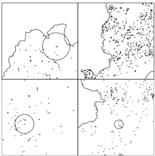
Figure 1: Maps of Belo Horizonte with four types of crime. The upper row shows the 765 drugstore robberies (left) and the 2216 bakery robberies (right). The bottom row shows the 582 lottery house robberies (left) and the homicides (right). The first three range from 1998 to 2000 while homi-cides data range from 1998 to 2001.
space-time clustering, bakery and drugstore robbery have
small p-values while the evidence for lottery robbery
de-pends on the threshold used and even then it is only border-line significant.
To run our scan procedure in the same dataset, we used a minimum of 5 events in each cylinder and we limit the cylinders to contain at most 15% of the observed events and
to not cover more than 15% of either the areaAor the total
time interval[0, τ]. We used 999 Monte Carlo simulations
to generate the null hypothesis distribution.
We foundC∗
1as a significant (at 0.05 level) space-time
cluster in all four crimes, with bakery robberies presenting
alsoC∗
2 as a significant cluster (see Table 1). The number
of events in the most significant cluster was 5, 7, 6, and 5 events for bakery, drugstore, lottery robberies, and homi-cide, respectively. The second significant cluster of bakery robberies had 5 events. Although the homicide space-time cluster presented borderline significance, we can see that the scan test identified clusters in homicide and lottery rob-beries, whereas Knox test did not. This suggests that our method could be more sensitive to the presence of localized clusters than Knox test.
Figure 2 presents the maps from Figure 1 zoomed to show the significant space-time clusters we detected with our scan procedure. The cluster covering the largest area was drugstore robbery with 1.52 kilometers of radius while the other clusters ranged from 370 to 760 meters. Hence, the events within the clusters are tightly clustered in space.
* * ** * * * * * * * * ** * * * * * * * * * * * * * * * * * * * ** * * * * * * * * * * * * * * * * * * * * * * * * * * * * * * * * * * * * * * * * * * * * * ** * * * * * * * * * * * * * * * * * * * * * * * * * * ** * * * * * * * * * * * * * * * * * * * * * * * * * * * * * * * * * * * * * * * * * * * * * * * * * * * * * * * * * * * * * * * * * * * * * * * * * * * * * * * * * * * * * * * * * * * * * * * * * * * * * * * * * * * * * * * * * * * * * * * * * * * * * * * * * * * * * * * * * * * * * * * * * * * * * * * * * * * * * * * * * * * * * * * * * * * * * * * * * * * * * * * * * * * * * * * * * * * * * * * * * * * * * * * * * * * * * * * * * * * * * * * * * * * * * * * * * * * * * * * * * * * * * * * * * * * * * * * * * * * * * * * * * * * * * * * * * * * * * * * * * * * * * * * * * * * ** * * * * * * * ** * * * ** * * * * * * * * * * * * * * * * * * * * * * * * * * * * * * * * * * * * ** * * * * * * * * * * * * * * * * * * * * * * * * * * * * * * * * * * * * * * * * * * * * * * * * * * * * * * * * * * * * * * * * * * * * * * * * * * * * * * * * * * * * * * * * * * * * * * * * * * * * * * * * * * * * * * * * * * * * * * * * * * * * * * * * * * * * * * * * * * * * * * * * * * * * * * * * * * * * * * * * * * * * * * * * * * * * * * * * * * * * * * * * * * * * * * * * * * * * * * * * * * * * * * * * * * * * * * * * * * * * * * * * * * * * * * * * * * * * * * * * * * * * * * * * * * * * * ** * * * * * * * * * * * * * * * * * * * * * * * * * * * * * * * * * * * * * * * * * * * * * * * * * * * * * * * * * * * * * * * * * * * * * * * * * * * * * * * * * * * * * * * * * * * * * * * * * * * * * * * * * * * * * * * * * * * * * * * * * * * * * * * * * * * * * * * * * * * * * * * * * * * * * * * * * * * * * * * * * * * * * * * * * * * * * * * * * * * * * * * * * * * * * * * * * * * * * * * * * * * * * * * * * * * * * * * * * * * * * * * * * * * * * * * * * * * * * * * * * * * * * * * * * * * * * * * * * * * * * * * * * * * * * * * * * * * * * * * * * * * * * * * * * * * * * * * * * * * * * * * * * * * * * * * * * * * * * * * * * * * * * * * * * * * * * * * * * * * * * * * * * * * * * * * * * * * * * * * * * * * * * * * * * * * * * * * * * * * * * * * * * * * * * * * * * * * * * * * * * * * * * * * * * * * * * * * * * * * * * * * * * * * * * * * * * * * * * * * * * * * * * * * * * * * * * * * * * * * * * * * ** * * * * * * * * * * * * * * * * ** * * * * * * * * * * * * * * * * * * * ** * * * * * * ** * * * * * * * * * * * * * * * * * * * ** * * * * * * * * * * * * * * * * * * * * * * * * * * *** * * * * * * * * * * * * * * * * * * * * * * * * * * * * * * * * * * ** * * * * * * * * * * * * * * * * * * * * * * * * * * * * * * * * * * * * * * * * * * * * * * * * * * * * * * * * * * * * * * * * * * * * * * * * * * * * * * * * * * * * * * * * * * * * * * * * * * * * * * * * * * * * * * * * * * * * * * * * * * * * * * * * * * * * * * * * * * * * * * * * * * * * * * * * * * * * * * * * * * * * * * * * * * * * * * * * * * * * * * * * ** * * * * * * * * * * * * * * * * * *
Figure 2: Zoomed maps of Belo Horizonte with the
signif-icant space-time clustersC∗
j by type of crime, in the same
order as Figure 1. Bakery robbery is the only crime with two significant space-time clusters, the others having only one significant cluster (at 0.05 value).
One store was robbed twice in each of the lottery and drug-store clusters. A more extreme pattern was found in the second bakery cluster with one store robbed three times. There were no obvious spatial pattern connecting clusters from different crimes.
Concerning time, the shortest bursts of spatially local-ized violence was that associated with the two clusters of
bakery robberies. They first and second clusters C∗
1 and
C∗
2 lasted 8 and 17 days starting on February, 28 2000 and
March 29, 2000 respectively. Drugstore and lottery rob-beries had longer clusters lasting 68 and 81 days starting on April 03, 1997 and May 23, 1995, respectively. The homi-cide cluster was detected on February 03, 2000, lasting 58 days.
The significant clusters of bakery robberies showed
extreme patterns. ClusterC∗
1 lasted only 8 days and,
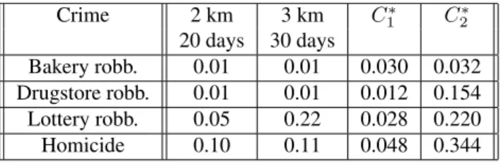
Crime 2 km 3 km C∗
1 C
∗ 2
20 days 30 days
Bakery robb. 0.01 0.01 0.030 0.032
Drugstore robb. 0.01 0.01 0.012 0.154
Lottery robb. 0.05 0.22 0.028 0.220
Homicide 0.10 0.11 0.048 0.344
Table 1: Table with the p-values of Knox and scan tests. The results are separated according to either the thresholds
used in the test (Knox) or the first (C∗
1) and second (C2∗)
most significant cylinders (scan test). The null hypothesis distribution was determined by 999 Monte Carlo
permuta-tions of the observed timesti.
5 Conclusion
Recently, there has been interest on space-time surveillance systems for the early detection of disease outbreaks, but very few studies have provided solutions to this problem. Rogerson (2001) proposed to use a cumulative sum approach for space-time point processes data, each event being scored according to a local Knox statistic. Theophilides (2003) uses multiple Knox test (1964) in multiple local area, so see whether one or more exhibit space-time clustering within that local area. Their method is very different from the one proposed here. Kulldorff et al. (2002,2003) have devel-oped a space-time permutation scan statistic for the early detection of disease outbreaks, which is currently in use by the New York City Department of Health for syndromic surveillance. They use a Poisson based likelihood ratio test statistic rather than the score test proposed in this paper. All of these methods are prospective in nature, in that they are looking for recent outbreaks, as opposed to our retrospec-tive method, which aims at detecting space-time clusters at any location and time.
In conclusion, our method has many desirable featu-res: it does not require population data; it identifies the space-time clusters; it does not require time and distance critical thresholds as Knox test does, it adjusts for purely spatial and purely temporal clustering, and it provides sta-tistical inference for each individual cluster detected. We think it will be of great use in many practical applications.
Acknowledgements
This work was partially supported by project SAUDAVEL, joint call MCT/SEPIN - FINEP - CNPq 01/2002. The data-set used in the example was kindly provided by the Pol´ıcia Militar de Minas Gerais.
Appendix: Algorithm Complexity
The algorithm has two steps. The first one finds the
rel-evant time and space cylinders and this takesO(nlogn)
andO(n2logn)complexity, respectively. The second step
finds the space-time cylinders as intersections of space and
time cylinders and this takesO(n4)running time.
There-fore, a single execution of the scan procedure takes
O(nlogn) +O(n2logn) +O(n4) =O(n4)
running time. It takesO(pn4)to obtain the null
hy-pothesis distribution with p independent permutations of
time indexes. In order to obtain thebnon-intersecting most
significant cylinders, we needO(b2n4)running times. We
describe these calculations with more detail.
Temporal and spatial ranks input
Lett(1) < t(2) < . . . < t(n) be the ranked values of the
observed times andmtbe the maximum length of a time
cylinder. The set of time cylindersCT induced by the
ob-served events is
CT ={(t(i), t(j))|i < jandt(j)−t(i)≤mt}.
We derive the time cylinders from the time ranked
val-ues and these are obtained inO(nlogn)running time if we
use optimal sorting algorithm, such asquicksort.
The set of relevant space cylindersCS is the union of
the space cylinders centered at eventse. Let(xe, ye)be the
center of a space cylinder andde
(2) < d
e
(3)< . . . < d
e
(n)be
the ranked distances of the other observed events to event
e. Note thatde
(1)= 0since it is the distance betweeneand
e. Ifmdis the maximum radius of a space cylinder, the set
of space cylindersCS is
CS =
n ³
xe, ye, de(s)
´
|e, s∈ {1, . . . , n}, s≥2, andde
(s)≤md
o .
The distance ranked values are sufficient to define
spa-ce cylinders. They can be evaluated by n sorting
algo-rithms. Therefore, we need O(n2logn) running time to
generate the spatial cylinders.
Scan procedure complexity
Given an evente, loopsSL2andSL3should guarantee the
generation of all time cylinders containingeand all space
cylinders centered ate. A time cylinder is generated by
defining first an allowable initial timetm =t(i)(tm ≤te
andte−tm ≤ mt), and then, a valid final time tM =
through events in their temporal ordering determiningiand
f inO(logn)time. LoopSL2is implemented by letting
m vary from i tillrt(e)where rt(e) is event e temporal
rank. For a fixedm, valid time cylindersCT = (t(m), t(M))
are those that containse (M varies from rt(e)tof) and
respects time thresholdmt. There are at mostPni=1(n−
i) < n2such cylinders (depending on them
tvalue), thus
SL2is performedO(n2)times. The size of a time cylinder
CT = (t(m), t(M))inSS2isM−m+ 1events and can be
evaluated in constant time.
For a fixed time cylinderCT, space cylinders
gener-ated in loopSL3should contain at least them-th andM-th
time events in order to minimize the re-generation of
space-time cylinders. LetemandeM be those events. The space
cylinder minimum radius isr= min{d(e, em), d(e, eM)}.
Letlbe the distance rank of this radius, which can be
deter-mined inO(logn). Spatial cylinders in loopSL3are of the
formCS ={(xe, ye, de(s))|l ≤s < g}, whered
e
(g)> md
or g = n+ 1. LoopSL3is performedO(n)times. The
evaluation ofN(CS)inSS2is exactlys, and takes constant
time.
The space-time cylinders are the intersection of events
in a spatial and a time cylinder. For a fixed CT in loop
SL2, spatial cylinders are considered in increasing radius
in loopSL3. Hence, a new spatial cylinder must include all
previous events and at least one additional event. Initially, a sequential scan is used to determine the intersection of
CT andCS = (xe, ye, de(l)), by comparing the timesteof
eventse ∈ CS to the time interval ofCT. For each new
CS, a new event is included and the comparison is repeated.
It results that the computation of all C in step SS3for a
loopSL3isO(n)(which is also the complexity ofN(C)).
OperationsN(CT),N(CS)and the test statisticsTCare all
O(1).
The resulting computational complexity of the
algo-rithm is the pre-processing time,O(nlogn)for time rank
andO(n2logn)for space rank, plus the space-time
cylin-ders generation which has complexity
|SL1|¡
O(logn) +|SL2|¡
O(logn)+ |SL3|[O(SS1) +O(SS2) +O(SS3)]¢¢
.
where —S— denotes the number of times loopS is
executed. From the previous discussion, |L1| = O(n),
|L2|=O(n2)and|L3|[O(S1) +O(S2) +O(S3)] =O(n).
Therefore, the final complexity of our scan algorithm is
O(n4).
Bibliography
Cliff AD, Ord JK (1981) Spatial processes: models and ap-plications. Pion Limited: London.
Cox DR, Hinkley DV (1974) Theoretical Statistics.
Chapman and Hall: London.
Diggle PJ, Chetwynd AG, H¨aggkvist R, Morris SE
(1995). Second-order analysis of space-time clustering.
Sta-tistical Methods in Medical Research, 4, 124-136.
Duczmal LH, Assunc¸˜ao RM (2003) A simulated an-nealing strategy for the detection of arbitrary shaped spatial
clusters. Computational Statistics and Data Analysis, in
press.
Jacquez GM (1996) Aknearest neighbor test for
spa-ce-time interaction.Statistics in Medicine, 15, 1935-1949.
Knox EG (1964) The detection of space-time
interac-tions.Applied Statistics, 13, 25-29.
Kulldorff M (1997) A spatial scan statistic,
Communi-cations in Statistics - Theory and Methods, 26 (6): 1481-1496.
Kulldorff, M (2001) Prospective time periodic
geo-graphical disease surveillance using a scan statistic.
Jour-nal of the Royal Statistical Society, Series A, 164, 61-72. Kulldorff M, Heffernan R, Hartmann J, Assunc¸˜ao RM, Mostashari F. A space-time permutation scan statistic for the early detection of disease outbreaks. Manuscript, 2003. Kulldorff M, Hjalmars U (1999) The Knox method
and other tests for space-time interactionBiometrics, 55 (2):
544-552.
Kulldorff M and IMS Inc. SaTSacan v3.0: Software for the spatial and space-time scan statistics. Available at [http://www.satscan.org], 2002.
Mantel N (1967) The detection of disease clustering
and the generalized regression approach.Cancer Research,
27, 209-220.
Rogerson PA (1997) Surveillance systems for
mon-itoring the development of spatial patterns. Statistics in
Medicine, 16, 2081-2093.
Rogerson PA (2001) Monitoring point patterns for the
development of space-time clusters. Journal of the Royal