Nonparametric dependence modelling for space-time cluster detection

Ricardo Fonseca Couto

NONPARAMETRIC DEPENDENCE

MODELLING FOR SPACE-TIME CLUSTER

DETECTION

Ricardo Fonseca Couto

NONPARAMETRIC DEPENDENCE

MODELLING FOR SPACE-TIME CLUSTER

DETECTION

Tese apresentada como requisito

parcial para obtenção do grau de

Doutor em Estatística

Banca Examinadora:

Orientador: Prof. Dr. Luiz Henrique Duczmal

Co-Orientadora: Prof. Dra. Denise Burgarelli Duczmal Membro: Prof. Dr. André Luiz Fernandes Cançado Membro: Prof. Dr. Gladston Juliano Prates Moreira Membro: Prof. Dr. Ricardo Hiroshi Caldeira Takahashi Membro: Prof. Dr. Roberto da Costa Quinino

Programa de Pós-Graduação

Departmento de Estatística

Universidade Federal de Minas Gerais

Agradecimentos

Primeiramente, sempre agradeço a Deus por toda a ajuda necessária. Sem Ele, nada acontece. E é Ele que nos cerca de pessoas que tornam o ambiente tão propício para o desenvolvimento pessoal e proĄssional.

O agradecimento às mulheres que me rodeiam não poderia deixar de ser especial: à minha mãe que, simplesmente, não tenho palavras para descrevê-la. Suporte total, irrestrito e incondicional. Às minhas irmãs, Mayra e Mylena, pelo desenvolvimento ao longo de todos estes anos, sendo alguns difíceis de vencer. Ao meu pai, Paulo Heslander, e ao irmão, Ronaldo, que sempre me incentivaram esta etapa nada elementar. À todos os meus familiares, cunhado, sobrinhos, tios, primos, que sempre estiveram do meu lado. Ao Martin Orji pelo incentivo e oportunidade deste sonho.

A todos os professores que são e serão para sempre nossos eternos mestres e aos colaboradores do Departamento, especialmente Rogéria e Rose, que me apoiaram intensamente.

Ao grupo de Equações Diferenciais Estocásticas: Luiz, Denise e Felipe. Mentes (e mais que isso, pessoas) brilhantes que tem a capacidade de motivar, compartilhar e cobrar de forma tão harmônica a tornar o trabalho cada vez mais prazeroso. Não consigo nem imaginar o que teria sido do doutorado sem essas pessoas tão diferenciadas no percurso. Fico feliz e honrado por fazer parte deste grupo tão seleto.

Aos colegas do curso, principalmente os frequentadores da sala de Pós-Graduação, que Ązeram parte do aprendizado de forma tão direta.

Gostaria de agradecer, por Ąm, de forma especial e muito carinhosa, a pessoa mais incrível que pude conhecer em toda minha vida: minha esposa, Lara, com quem tive o orgulho de casar durante o curso. Posso dizer que sou a pessoa mais privilegiada por ter uma mulher tão especial ao meu lado todos os dias. Ao Marco Polo, à Sônia e ao Gabriel, por tudo que representam para mim.

Resumo

Estruturas de dependência são estudadas exaustivamente em diversas aplicações. Nesta tese, uma nova metodologia para a detecção de clusters, chamada de Distância Ponder-ada de Voronoi, é apresentPonder-ada levando em consideração não somente a localização dos pontos, mas também sua estrutura temporal. Usando o espaço de variáveis ao invés da localização geográĄca, como em estatística espacial, e o toro em lugar do plano cartesiano, esta metodologia permite que o usuário aplique a ideia para um número maior de cenários alternativos. Em particular nos mercados Ąnanceiros, diferentes modelagens de dependência entre ativos podem levar a mudanças drásticas na alocação de recursos e a diferentes exposições a risco. Além disso, estas relações de dependência podem ser utilizadas como mecanismos para a detecção de crises Ąnanceiras mais rápidos que os modelos fundamentalistas, através do efeito contágio. Inicialmente, esta aplicação é realizada entre ativos de um mesmo mercado, o mercado americano, comparando a metodologia proposta com metodologias mencionadas na literatura como coeĄcientes lineares e copulas. Esta abordagem foi estendida para ativos de mercados distintos, a Ąm de se analisar a disseminação de crises Ąnanceiras entre diferentes mercados. Resultados obtidos através de simulações e aplicações com dados reais mostraram melhorias se comparados com abordagens clássicas, especialmente em períodos Ąnanceiros turbulentos.

Abstract

The dependence structures have been exhaustively studied in many applications. In this thesis, a new methodology for cluster detection is presented, i.e. the Weighted Voronoi Distance (WVD), taking into consideration not only the location of the points but also their time structure. Using variables space instead of geographical location as in spatial statistics and the torus instead of a regular Cartesian plane, this methodology allows the user to apply the rationale for more alternative scenarios. Particularly in Ąnancial markets, different dependence modelling among assets can lead to signiĄcant changes in asset allocation and different risk exposures. Besides, these dependence relationships can be used as mechanisms to detect Ąnancial crisis more quickly than fundamental models through the contagion effect. Initially, this application is run using assets from the same market, i.e. the US market, comparing the proposed methodology with methodologies mentioned in literature such as linear coefficients and copulas. This approach will be extended to assets from distinct markets in order to analyse the Ąnancial crisis dissemination across different markets. Results obtained from simulations and real data applications showed improvements compared to classical approaches especially in during turbulent Ąnancial periods.

Contents

List of Figures vi

List of Tables vii

Apresentação vii

1 Introduction 3

2 Dependence Modelling using Copulas 6

2.1 Copulas . . . 6

2.1.1 Elliptical Copulas . . . 7

3 Dependence Modelling Measures and Cluster Analysis and

Detec-tion 9

3.1 Cluster Analysis . . . 9

3.1.1 Weighted Voronoi Distance . . . 9

3.1.2 Cluster Detection and WVD Space-Time Scan . . . 10

4 Simulation Study 14

4.1 Discussion . . . 17

5 Financial Markets and the Weighted Voronoi Distance Space-Time

Scan 19

5.1 Financial Market Crisis . . . 19

5.2 The US Financial Market Crisis and the WVD Space-Time Scan . . . . 22

5.3 International Financial Markets and the WVD Space-Time Scan . . . . 25

6 Conclusions and Final Remarks 29

List of Figures

3.1 Example of Weighted Voronoi Distance (WVD) . . . 10

3.2 Example of possible clusters . . . 11

3.3 Cluster in Cartesian plane and in torus . . . 13

4.1 Scatter plot for alternative scenarios. . . 15

4.2 Sliding window for cluster detection. . . 16

5.1 Daily returns. . . 22

5.2 Scatter plot and the torus representation. . . 23

5.3 P-values for different assets in the US market. . . 24

5.4 Correlation coefficients estimated by EVT and Copula for ARMA/GARCH Ąltered series (US market). . . 26

5.5 P-values for different assets in international markets. . . 27

List of Tables

4.1 Critical Values for the Empirical Distributions. . . 16

4.2 Simulation Results. . . 17

5.1 P-values for the US market. . . 23

Apresentação

A relação de dependência entre variáveis aleatórias é motivo de estudo há séculos. Inicialmente, medidas de associação lineares foram desenvolvidas e, com o passar do tempo, medidas não lineares foram apresentadas. Paralelamente, os estudos de séries temporais também se tornaram difundidos na análise que incorporam os efeitos do tempo no comportamento de uma variável aleatória. Entretanto, no mundo real, podemos encontrar variáveis aleatórias que estão, de alguma forma associadas, mas também possuem o efeito da variável tempo tanto dentro das próprias séries como entre elas. Como entender este comportamento? É possível veriĄcar de forma rápida e eĄciente um aumento ou diminuição da dependência destas variáveis para pequenas variações?

Sendo encontrada em diversas áreas do conhecimento, estas questões apontadas acima são de extrema importância para o entendimento de fenômenos e tomadas de decisão. Por isso, esta tese foi desenvolvida através do estudo de estruturas de dependência entre variáveis aleatórias, culminando na proposta de uma nova medida de dependência. Esta abordagem possui algumas vantagens sobre as abordagens já apresentadas na literatura: (i) possibilita a utilização de dados em tempo real, (ii) intrinsecamente traz a estrutura temporal das séries, (iii) se baseia em técnicas de estatística espacial próprias para a deteccção de clusters, deĄnidos formalmente no Capítulo 1 e (iv) utiliza uma topologia capaz de suportar uma variedade maior de modelos alternativos.

List of Tables 2

Chapter 1

Introduction

Dependence between two variables has been of major concern in many Ąelds not only for statisticians but also for both researchers and practitioners from biological to social sciences. Along the last centuries, independently of any particular application, many measures have been proposed. Although the linear correlation coefficient (PearsonŠs ρ)

proposed by Pearson (1895) is the most popular, other concordance measures such as rank correlation have been introduced to better apprehend correlation drawbacks. Spear-man(1904) proposed a concordance measure (as known as ŞSpearmanŠsρŤ) which does

not assume linear relationships among variables but only monotonicity. Kendall (1938) has also proposed a concordance measure, the ŞKendalŠsτŤ, with similar characteristics

and assumptions.Pantaleo et al. (2011), for instance, show a comparative study of nine covariance matrix estimators and Deng and Tsui(2013) propose a different method to estimate the covariance matrix using matrix-logarithm transformation, to cite only a few. One of the main issues about the covariance matrix is due to its non-static nature. Many studies discuss the dynamic behaviour of the covariance matrix and provide alternative methods and metrics to estimate and evaluate the change taking into account the time structure (Andersen et al., 2009; Bauwens et al., 2006; Engle,

2002)

4

However, data time structure such as autocorrelation and homoskedasticity were not taken into consideration in these studies. For time series analysis, other tools have been developed separately such as Auto Regressive Conditional Heteroscedas-ticity/Generalized Auto Regressive Conditional Heteroskedasticity (ARCH/GARCH) developed by Engle (1982) and Bollerslev (1986), and its derivations, for instance, Asymmetric Power ARCH (Ding et al.,1993), Exponential GARCH (Nelson, 1991), and Multivariate GARCH (Bauwens et al.,2006).

Recently, many studies have been published using copulas and conditional volatility to explain the contagion effect in Ąnancial markets (Brunnermeier and Perdersen,

2005; Forbes and Rigobon,2002; Kaminsky et al., 2003; Naoui et al., 2010; Rodriguez,

2007). Particularly in Ąnancial applications, thecontagion effect is when the returns of Ąnancial assets show increase in their dependence structure or, graphically speaking, appear in a unlikely manner around the regression line. An important aspect of this phenomenon is that the high positive returns can also be correlated with high negative returns as in Ąnancial ŞbubblesŤ. In quantitative Ąnance, both risk management and asset allocation procedures rely strongly upon dependence measures to estimate risk factors and achieve efficient diversiĄcation. As stock returns show asymmetric lower and upper tail dependence, the behaviour cannot be captured by traditional linear correlation coefficient (Ang and Bekaert, 2002; Granger and Silvapulle, 2001; Login and Solnik,2001).

Copula functions also turn out to play an important role in dependence modelling especially due to concordance characteristics, capacity to model tail dependence and Ćexibility to work in a non-Gaussian world. However, in order to use the Extreme Value Theory (EVT) and Generalized Pareto (GP) distribution model for both left and right tails separately, the independence and identically distribution (i.i.d) assumptions cannot be broken. Therefore, an ARMA/GARCH approach is usually applied to generate the Ąltered conditional residuals which can be assumed to be independent and identically distributed (Ghrobel and Trabelsi, 2009; Nystrom and Skoglund,2002). Besides, copula selection and validation tools are not unanimous. For instance, Huard et al.(2006) considered copulas selection without counting for marginal modelling.Silva and Lopes (2008) show advantages of estimating all parameters and used the deviance information criterion, proposed by Spiegelhalter et al. (2002).Michiels and Schepper

5

Formally, a spatial cluster is the localized portion of the domain which contains a higher-than-average proportion of cases over controls, and a space-time cluster can be deĄned as unexpected concentrations of cases in a time series sequence of maps. One of the predecessors in this Ąeld was Kulldorff (1997) who developed a spatial scan statistics to detect a geographical cluster as early as possible. Thereafter, Kulldorff

(2001) proposed a prospective time scan method improved by Duczmal et al. (2006). Other methods such as Conley et al. (2005), Wieland et al. (2007), Yiannakoulias et al. (2007) and Duczmal et al. (2008) have also been presented to detect clusters using different techniques. Duczmal et al. (2011) showed an extension for a prospective space-time scan called the Voronoi Based Scan which uses the spatial tessellation and Voronoi cells boundaries to detect clusters.

Although, at a Ąrst glance, these problems seem to be unrelated, the rationale behind them is quite similar. Suppose X, Y are two random variables with an

un-known dependence structure between them. Without assuming any condition for the relationship such as linearity or lack of sample autocorrelation, the main interest is to analyse the time behaviour of the dependence structure which can be used for many applications such as cluster detection in spatial statistics and contagion effect signalling in Ąnancial markets. As described in Dornbusch et al. (2000), the Ąnancial contagion detection can serve as a tool to anticipate a crisis in Ąnancial markets.

This work proposes a new non-parametric methodology based upon a non-ordinary metric: the Weighted Voronoi Distance (WVD). Although extensive theoretical dis-cussion can be found in Okabe et al. (2000) about spatial tessellation which has been widely used in many Ąelds such as biology and physics, it has not been used, to the best of our knowledge, to model the space-time dependence structure between two random variables. The main goal is to use the technique to develop a method able to detect the increase in dependence more quickly than traditional measures. To illustrate the potential advantages, simulations were run and real Ąnancial datasets were used to verify how quick the 2007 subprime crisis could have been warned.

Chapter 2

Dependence Modelling using

Copulas

Copulas are the cutting edge technique to analyse the dependence structure today due to its characteristics and Ćexibility (Boubaker and Sghaier, 2013;Meucci, 2011;

Patton, 2012). Therefore, this Chapter deĄnes this measure in section 2.1, mentioning the practical issues and beneĄts of such mathematical tool.

Broadly speaking, two parametric copula families are the most common and men-tioned in literature, i.e. the elliptical and Archimedean copulas. In this work, the elliptical family will be described and used as parameters interpretation is eased through the transformation to traditional ρ. Furthermore, for Archimedean families, not only

are such analytical transformations not possible making it harder to interpret the parameters, but they also have showed poor results for Goodness-of-Ąt test for Ąnancial series (Patton, 2012).

2.1

Copulas

The wordcopula has its origin in Latin meaning ŞbondŤ or ŞtieŤ. In statistics, Sklar (1959) was the Ąrst to mention this particular word in a theorem which bears his name (pointed out in this section). Since then, this measure has become of great interest among statisticians especially due to its scale-free characteristics and the possibility of constructing families of bivariate distributions.

Formally, letI = [0,1]. Then, copulas can be deĄned as:

Definition 2.1.1 A two-dimensional copula is a function C:I2 _{→I such that:}

2.1 Copulas 7

(ii) for all a, b, c, d∈I, with a≤b and c≤d,

Vc([a, b]x[c, d]) = C(b, d)−C(a, d)−C(b, c) +C(a, c)≤0. (2.1)

The functionVc is also called theC−volumeof the rectangle [a, b]×[c, d].

Equiva-lently, a copula is a bivariate distribution whose margins are uniform in [0,1] restricted

to the unit square [0,1]×[0,1].

The importance of copulas in statistical Ąeld has been increasing due to SklarŠs Theorem.

Theorem 2.1.1 (Sklar’s Theorem) Let G be a two-dimensional distribution function with marginal distribution functions F1 and F2. Then there exists a copula C such that

G(x, y) =C(F1(x), F2(y)). Conversely, for any distribution functions F1 and F2 and

any copula C, the function G defined above is a two-dimensional distribution function with marginals F1 and F2. Furthermore, if F1 and F2 are continuous, C is unique.

According to SklarŠs theorem, using a collection of copulas it is possible to construct bivariate distributions with arbitrary margins. Nelsen (2006) and references therein describe in details many parametric families and their characteristics. Normal and t copulas and the Farlie-Gumbel-Morgenstern (FGM) copula family are widely used in literature as mentioned byAas (2004); Kolev and Paiva (2009); Manner and Reznikova

(2012); Patton(2012) to mention only a few. However, the FGM family can only model relatively weak dependence (Nelsen, 2006). Thus, the immediate interest is to focus on Normal and t copulas.

2.1.1

Elliptical Copulas

Let Φρ be the standard bivariate normal joint distribution with correlation coefficient

ρ. Then, the Normal (or Gaussian) copula is given by: CN

ρ (u, v) = Φρ(Φ−1(u),Φ−1(v)) (2.2)

where Φ−1 _{denotes the standard normal distribution function. It is worth mentioning}

that since there is no analytical expression for Φ−1_{, Φ}

ρ has also no closed form.

The t (or Student) copula can be deĄned analogous to the normal copula. Let

Tv,ρ be cumulative bivariatetv,ρ distribution with correlation coefficient ρ. Then, the

t-copula is given by:

CT

2.1 Copulas 8

Although both copulas have similarities, their behaviour in case of extreme events (when the interest is to see the joint extremes) differ substantially. In order to study the tail behaviour, the upper and lower tail dependences (λU and λL, respectively) can

be deĄned as:

λU = lim

t↗1P(Y > F

−

2 (t)♣X > F1−(t))

= 2−lim

t↗1

1−C(t, t) 1−t λL= lim

t↘0P(Y ≤F

−

2 (t)♣X ≤F1−(t))

= lim

t↘0

C(t, t)

t

(2.4)

It is possible to show that the Gaussian copula has 0 tail dependence for any given correlation ρ. However, t-copula has its upper and lower tail dependence evaluated by:

λt

v,ρ= 2tv+1





−[(1 +v)(1−ρ)]12

(1 +ρ)12



 (2.5)

Chapter 3

Dependence Modelling Measures

and Cluster Analysis and Detection

In this Chapter, the main contribution of this thesis is presented. First of all, the new measure, called Weighted Voronoi Distance, is deĄned followed by a cluster detection algorithm and a Space-Time Scan based on it.

3.1

Cluster Analysis

3.1.1

Weighted Voronoi Distance

The Ąrst step to build the proposed metric is to deĄne Voronoi diagram. Considern

point in the space domain and the set P = ¶(xi, yi) :i= 1, ..., n♦ ⊂ ℜ2. For i= 1, ..., n,

the Voronoi cell v(i) consists of those points inℜ2 _{which are closer to (x}

i, yi) than any

other point in P. The Voronoi diagram is the collection of cells v(i), i= 1, ...n.

Let vk be a Voronoi cell which is crossed by the line segment joining points

ci = (xi, yi) and cj = (xj, yj), dk the length of the segment that is in vk, and ak the

area of the cell vk. Then, the Weighted Voronoi Distance (WVD) is deĄned as:

W V Dci,cj =

nk

X

k=1

(dk/ak) = nk

X

k=1

(wk∗dk) (3.1)

wherenk is the total number of cells crossed by the line segment and wk = 1/ai is

3.1 Cluster Analysis 10

−4 −3 −2 −1 0 1 2 3 4

−4 −3 −2 −1 0 1 2 3 4

Cell 1 Cell 2

Cell 3

Cell 4 _{Cell 5} Cell 6

Cell 7

Cell 8 Cell 9

Cell 10 Cell 11 Cell 12 Cell 13 Cell 14 Cell 15 p q 1 2 3 4

Fig. 3.1 Example of Weighted Voronoi Distance (WVD).

Example 3.1.1 Let p and q be two points in the plane illustrated in Figure 3.1. The formula becomes:

W V Dp,q =

4

X

i=1

di/ai =d1/a1+d2/a2+d3/a3+d4/a4 (3.2)

The numbered segments, di, emphasize that each segment is weighted by its Voronoi

cell area ai.

3.1.2

Cluster Detection and WVD Space-Time Scan

Having deĄned the WVD, it is possible to build a cluster detection procedure. Firstly, a data set called training set (T) (known as ŞcontrolsŤ in some Ąelds) is chosen, the Voronoi diagram is calculated and plotted with these points and the WVD is calculated for all possible pairs. Notably, as the metric is symmetric only (n2−n)/2 distances have

to be calculated, reducing the complexity of the algorithm. Besides, this training setT

has to be chosen to represent a randomly distributed population. Secondly, a Monte Carlo simulation is run m times to build the empirical distribution of WVDŠs. Then,

3.1 Cluster Analysis 11

as deĄned in Chapter 1, through an one-tail hypothesis test. The procedure can be summarized as:

1. Choose the Training Set (T) which describes the randomly distributed population

and calculate the Voronoi Diagram for these points.

2. Calculate the Weighted Voronoi Distance (WVD) for all pairs in the Training Set (T).

3. Build an Empirical Distribution for the WVD using Monte Carlo simulations. 4. Calculate the Weighted Voronoi Distance for the Candidate Set (C).

5. Compare the WVD of the Candidate Set with the appropriate percentile given the conĄdence level.

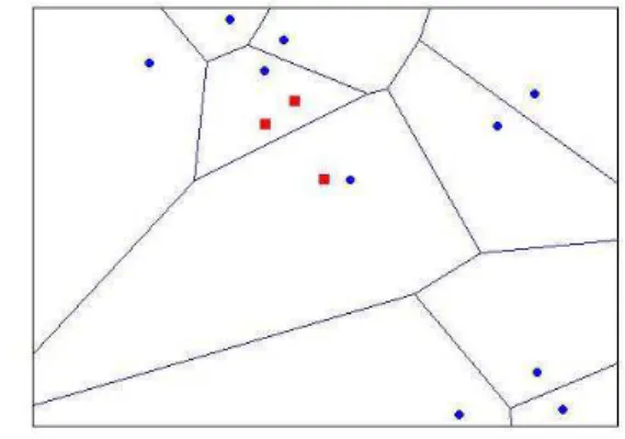
To visualize both the Training Set (T) and the Candidate Set (C), Figure3.2shows

an example of a Training Set with 10 points and a Candidate Set with 3 elements.

Fig. 3.2 The circles are the training set. The squares are the candidates for a cluster. It is worth mentioning that the points can hardly be identiĄed as signiĄcantly concentrated just looking at the map.

Formally, let ci be the i−th point, the training set T = Sni=1T ci, and nc be the

length of the candidate set C. Then, the W V Di of a subset of T = c(i−nc), ..., ci is

deĄned as:

W V Di = i

X

t=i−nc+1

3.1 Cluster Analysis 12

And the Empirical Distribution (ED) for a particular time length (or horizon)nc

obtained running m Monte Carlo simulations is deĄned as:

ED=

m

[

i=1

W V Di (3.4)

Having set the signiĄcance level, α, the one-tail hypothesis test is run:

  

 

H0 :W V Di ≥100∗αthpercentile(ED)

H1 :W V Di <100∗αthpercentile(ED)

One of the advantages of this new metric is that as it has been built upon the real line, it allows no multiple solutions, a problem faced by Duczmal et al. (2011).

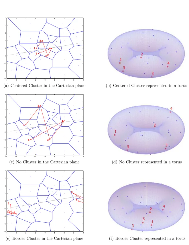
Particularly in Ąnancial applications, the contagion effect can be seen when the returns of Ąnancial assets increase their correlation getting closer to the regression line. As high positive returns can be followed by high negative returns as in Ąnancial unstable periods, instead of applying the WVD methodology for the original plane, i.e. returns of asset y against returns of asset x, a torus is created with its external longitudinal axis being the regression line of the original plane, maintaining the returns dependence characteristics. Furthermore, this geometry construction extinguishes the border problem when dealing with Voronoi Diagrams in classical Cartesian plane as borders are connected and no inĄnite border is necessary.

In Figure3.3 the original returns series are plotted for three different situations: a centered cluster, no cluster, and a border cluster.

3.1 Cluster Analysis 13

−4 −3 −2 −1 0 1 2 3 4

−4 −3 −2 −1 0 1 2 3 4 1 2 3 4 5

(a) Centered Cluster in the Cartesian plane (b) Centered Cluster represented in a torus

−4 −3 −2 −1 0 1 2 3 4

−4 −3 −2 −1 0 1 2 3 4 1 2 3 4 5

(c) No Cluster in the Cartesian plane (d) No Cluster represented in a torus

−4 −3 −2 −1 0 1 2 3 4

−4 −3 −2 −1 0 1 2 3 4 1 2 3 4 5

(e) Border Cluster in the Cartesian plane (f) Border Cluster represented in a torus

Chapter 4

Simulation Study

After describing the new methodology in Chapter 3, this chapter shows results and discussion about the methodology simulations under different scenarios, and comparison with copula approach.

For both methods, a training set (T) assumed to be the null hypothesis of 504

observations was generated from a bivariate Normal distribution with zero mean, 0.10 standard deviation for each variable, and 0.70 correlation coefficient between them. Formally, the empirical distribution is given by:

X H0

∼ N(µ,Σ), (4.1)

whereµ= [0,0] and Σ =h0.010 0.007 0.007 0.010

i .

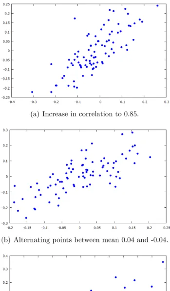
As alternative scenarios, three different changes in behaviour were tested. Firstly, the mean was kept at zero and the correlation was increased to 0.85. This scenario simulates the simple increase in correlation between two random variables. The second scenario was generated from distribution with the same covariance as the null hypothesis, but the mean for each sample was either [0.04,0.04] or [−0.04,−0.04]. The decision

as taken from a Bernoulli Distribution with pparameter equals to 0.5. Thus, keeping

the correlation constant, this scenario is expected to verify the detection capacity of the proposed algorithm in a situation where regular tools usually do not work as well as in the Ąrst scenario. Finally, the third scenario was generated changing the mean vector to µ = [−0.04,−0.04]. These cases were especially chosen due to practical

applications were this phenomena are found such as Ąnancial markets (described in details in Chapter 5). The alternative scenarios are shown in Figure 4.1.

15

(a) Increase in correlation to 0.85.

(b) Alternating points between mean 0.04 and -0.04.

(c) Translated points around (-0.04,-0.04)

16

last few observations, purely spatial analysis for the whole period dilutes the cluster strength and diminishes the power to detect such cluster. Conversely, for short periods, adjustments for multiple testing should be made when repeated analysis every month are taking place. Therefore, simulations were run using four different time periods, i.e.

n = 21, 42, 63 and 84 points, and tests were made after each step to check possible

cluster detections.

For each horizon, the WVD Space-Time Scan compares the Voronoi Distance with an empirical distribution as deĄned in equation 3.4. In each simulation, a collection of

n points was randomly selected from the 504 original points and Voronoi tessellation,

respecting their order, and the total Weighted Voronoi Distance was recorded. This step was repeated 100,000 times to build the empirical distributions for each horizon. With the empirical distributions, it was possible to calculate the critical values for each horizon and for different signiĄcance levels: 0.5%, 1%, 2%, 5%, 10%, 20%, 50%, and 80%. Table 4.2describes these values which play an important role in the proposed test.

Table 4.1 Critical Values for the Empirical Distributions for different horizons.

Significance Level Horizons

21 42 63 84

0.5% 7213.7 17144.7 27693.7 37634.0

1.0% 7596.2 17711.2 28333.2 38855.2

2.0% 8046.1 18333.3 29157.6 39818.6

5.0% 8662.4 19229.8 30165.1 41026.8

10.0% 9220.7 20027.4 31128.5 42195.4

20.0% 9868.7 20979.4 32314.3 43614.0

50.0% 11127.4 22863.4 34590.8 46306.2

80.0% 12433.5 24682.9 36933.2 48999.4

4.1 Discussion 17

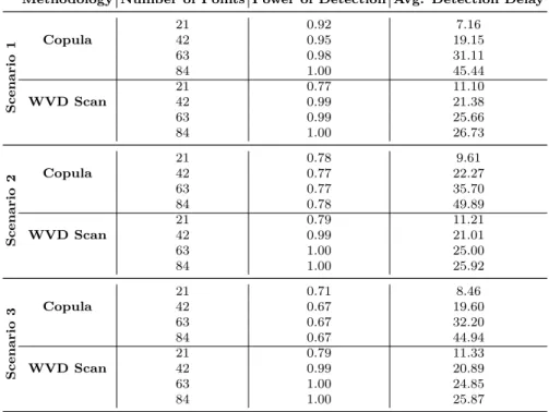
Table 4.2 Simulation results for different time horizons (95% conĄdence level).

Methodology Number of Points Power of Detection Avg. Detection Delay

Scenario

1

21 0.92 7.16

Copula 42 0.95 19.15

63 0.98 31.11

84 1.00 45.44

21 0.77 11.10

WVD Scan 42 0.99 21.38

63 0.99 25.66

84 1.00 26.73

Scenario

2

21 0.78 9.61

Copula 42 0.77 22.27

63 0.77 35.70

84 0.78 49.89

21 0.79 11.21

WVD Scan 42 0.99 21.01

63 1.00 25.00

84 1.00 25.92

Scenario

3

21 0.71 8.46

Copula 42 0.67 19.60

63 0.67 32.20

84 0.67 44.94

21 0.79 11.33

WVD Scan 42 0.99 20.89

63 1.00 24.85

84 1.00 25.87

As results were similar for all other signiĄcance levels, the analysis will be made for the 95% conĄdence level and tables for the remaining levels can be found in the Appendix.

4.1

Discussion

Having proposed the new methodology for cluster detection and run simulations for three different alternative scenarios for both Copulas and WVD Space-Time Scan, it is possible to compare both methodologies.

First of all, both methods behaved similarly for the scenario where the increase in dependence occurs through an increase in off-diagonal terms of the covariance matrix. Such a situation was expected for copulas as a direct transformation can be made to work with the linear correlation coefficient in question. On the other hand, for the same scenario, the WVD approach was also able to capture the data structure change and signalize the increase in dependence.

4.1 Discussion 18

Chapter 5

Financial Markets and the

Weighted Voronoi Distance

Space-Time Scan

This chapter describes the behaviour of global Ąnancial markets during crisis (section5.1

and applies the methodology proposed in Chapter 4 to detect clusters in Ąnancial assets returns. A comparison with copula methodology described in Chapter3 is made and the results are shown in sections 5.2 and 5.3.

5.1

Financial Market Crisis

5.1 Financial Market Crisis 20

Traditionally, it is believed that continuous long-term deterioration of macroeco-nomic factors would lead to Ąnancial crisis. Krugman(1979) is one of the predecessors in this Ąeld having studied how governments should not be able to sustain a pegged exchange rate regime using their foreign reserves to offset markets movements. Other-wise, a ŞcrisisŤ would be created in the balance of payments.Obstfeld(1986) innovated studying the self-fulĄlling balance of payments crises using stochastic models to link macroeconomic variables to the phenomenon. For decades, the early warning systems (EWS) for Ąnancial crisis were based on macroeconomic fundamentals and were

de-signed to monitor and predict the events in the mid- to long term, i.e. at least one year. However, due to lack or delay of information and relative low frequency of data releases, these models tend to respond slowly to market changes, although Ąnancial data demonstrate high variability.

Recently, many studies have been published trying to analyse and explain the spillover phenomena (Bae et al., 2003;Dungey et al.,2003; Forbes and Rigobon, 1999;

Kaminsky et al.,2003;Valdés, 1996). Dornbusch et al. (2000) and Pericoli and Sbracia

(2003), for instance, divided the transmission mechanisms into two different categories, i.e. interdependence and contagion. The Ąrst category is due to normal interdependence such as geographical position and trade links. This market interaction is based upon fundamentals and is responsible for the comovements in both tranquil and turbulent times. Calvo and Reinhart(2003) named this effect as Şfundamentals-based contagionŤ. The second category is another type of dependence which can be seen only in turbulent periods. Dornbusch et al. (2000) argues that this ŞirrationalŤ phenomenon is based on panic, loss of conĄdence and herd behavior, but not on Ąnancial nor macroeconomic variables. Kyle and Xiong (2001) and references therein discuss how effects other than fundamentals can and actually interfere in market behaviors.

The Ąnancial literature describes many mechanisms through which the contagion can be disseminated (Longstaff,2010, and references therein). First, the negative shocks in one market is associated with negative news that is directly linked to securities, for example, cash-Ćow and/or collateral, in other markets. Kaminsky et al.(2003); King and Wadhwani (1990);Kiyotaki and Moore (2002) are only a few authors who discuss these market news absorption from different perspectives. Second, Allen and Gale

5.1 Financial Market Crisis 21

to bear risk. Acharya and Pedersen (2005); Longstaff (2004); Vayanos (2004) show how distressed securities may be predictive of subsequent negative returns in other securities, leading to increase in risk premia asked by investors.

Econometric models have been developed to describe and forecast the economic phenomenon in question.Eichengreen et al.(1996) andFrankel and Rose(1996) showed almost simultaneously how currency crisis can be estimated using logit/probit models. Although they used different input variables and different deĄnitions for ŞcrisisŤ, the rationale is still very similar. Hawkins and Klau (2000) built Şvulnerability and pressure indicesŤ based on representative variables presented in the literature and achieved satisfactory results. Edwards (1998) studied the role interest rates play in crisis contagion in open economies using the generalized autoregressive conditionally heteroskedastic (GARCH) approach. The contagion effect among East Asian countries was modeled by Khalid and Kawai(2003) using vector autoregressive (VAR), and no strong support for contagion was found for the period and markets included. Longstaff

(2010) used the same approach for ABX subprime indexes and found strong evidence of contagion in the American Ąnancial market. Another leading modelling category is the non-parametric approach which utilizes available daily Ąnancial data to improve crises detection capability. Kaminsky et al. (1997) popularized the idea of deĄning threshold values beyond which a crisis would be said to take place using equity prices as one of the indicators. Thereafter, many other studies have been conducted in this line and moderately success has been obtained (Frankel and Saravelos,2010), although their focus were not crisis prediction but rather an ex-post analysis.

5.2 The US Financial Market Crisis and the WVD Space-Time Scan 22

Fig. 5.1 Daily Returns for all 4 asset series between 01/03/2003 and 12/31/2007.

5.2

The US Financial Market Crisis and the WVD

Space-Time Scan

The analysis of the American Ąnancial market was based upon daily returns of EURO, NASDAQ, iShares iBoxx Investment Grade Corporate Bonds and S&P500 were used from January, 3th_{, 2003 until December, 12}th_{, 2007, totalling 1253 samples for each}

series. The data was downloaded from Yahoo! Finance (Ąnance.yahoo.com) and the returns are plotted in Figure 5.1.

It was not until August, 2007, that the Federal Reserve officially published the turmoil in Ąnancial markets (FOMC,2007). Although authorities came to public only in the third quarter of 2007, investors and other market participants have already reacted to and priced the upcoming crisis, changing the behaviour and consequently the dependence structure between assets.

Figure5.2 shows on the left hand side the scatter plot for the returns around the

x-axis, i.e. the returns rotated by the regression line angle. On the right hand side,

the respective torus representation is shown. As similar results were obtained for all four pairs of assets, the illustration below is just for one particular case (Corporate Bonds and S&P500).

surveil-5.2 The US Financial Market Crisis and the WVD Space-Time Scan 23

Fig. 5.2 Scatter plot and the torus representation for Corporate Bonds and S&P500. Table 5.1 P-values for three different dates and four horizons.

Horizon 12/06 06/07 10/07

Corporate Bonds/S&P 1 month 0.04 0.97 0.00

2 months 0.00 0.93 0.00 3 months 0.19 0.87 0.00 4 months 0.12 0.00 0.00

Euro/Nasdaq 1 month 0.40 0.90 0.02

2 months 0.04 0.87 0.00 3 months 0.11 0.96 0.04 4 months 0.54 0.00 0.06

Euro/Corporate Bonds 1 month 0.08 0.50 0.02

2 months 0.04 0.74 0.00 3 months 0.22 0.80 0.03 4 months 0.16 0.00 0.14

Euro/S&P 1 month 0.43 0.76 0.32

2 months 0.02 0.59 0.04 3 months 0.06 0.74 0.13 4 months 0.37 0.00 0.35

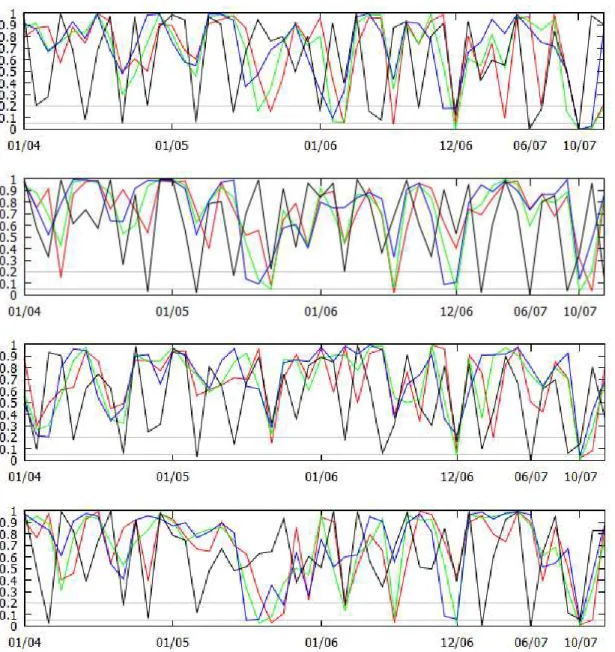
lance is used with one, two, three and four months. Figure 5.3 presents the p-values for 10,000 Monte Carlo simulations (m = 10,000).

Working with a 95% conĄdence interval, it is expected to Ąnd random points below both the 20 and 5% levels (horizontal lines). However, in December 2006, June 2007 and October 2007, all asset pairs presented at least one horizon below the 5% level. This effect can indicate a presence of a market reaction, a Ąnancial contagion, before the crisis announcements and earlier than previous studies about Early Warning Systems (Addo et al. 2013, for example). The p-values for these horizons are presented in Table

5.1.

Having analysed the results for the proposed model, we would like to compare the WVD Space-Time Scan with the Copula approach estimated by Ąltered conditional residuals obtained from a ARMA/GARCH model as shown by Nystrom and Skoglund

5.2 The US Financial Market Crisis and the WVD Space-Time Scan 24

5.3 International Financial Markets and the WVD Space-Time Scan 25

series. The second step was to estimate the empirical cumulative distribution function (CDF) for each series with a Gaussian kernel to smooth the interior the sample CDF pattern. Each tail, consisting of 15% of the residuals, was associated with a parametric Generalized Pareto Distribution (GDP) and their index (ζ) and scale

(β) parameters were estimated optimizing the log-likelihood function. Finally, the

standardized residuals are transformed to uniform variates and a t-copula (as described in 2.1) is Ątted to the transformed data. Figure 5.4 shows theρ for the pairs studied.

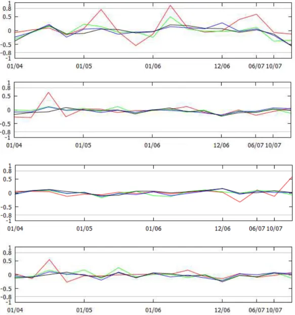
The horizontal lines in Figure5.4show a possible threshold for the coefficient of 0.8 and -0.8. It is worthy mentioning that the interpretation of the correlation coefficient graph is different from the p-values shown in Figure 5.3: while the crisis signal is given by a low p-value level in Figure 5.3, in Figure 5.4 the crisis is signalized by a high correlation coefficient. As can be seen, the positive threshold, i.e. +0.8, was crossed just once, in the Ąrst quarter of 2006, by the Corporate Bonds and S&P500 (1-month) series during the period in question. This signal is weaker than the signal generated by the WVD Space-Time Scan procedure.

5.3

International Financial Markets and the WVD

Space-Time Scan

In order to analyse the behaviour of the WVD Space-Time Scan for the international markets, equity indexes were used from the US, UK, and Japanese markets: S&P500, FTSE100, and NIKKEI225, respectively. These markets were chosen due to their representativeness in global Ąnancial markets and their informational efficiency.

The period in question was from January 2003 until December 2007 for all assets. However, the number of observations are different for each pair of series as only trading days were taken into account. The American and British pair was built with 1250 observations, the American and Japanese series had 1184 observations, and the Japanese and British pair showed 1223 observations.

Similar analysis as described in previous section is made and the p-values are shown in Figure 5.5 and Table 5.2.

5.3 International Financial Markets and the WVD Space-Time Scan 26

5.3 International Financial Markets and the WVD Space-Time Scan 27

Fig. 5.5 P-values for NIKKEI250 and FTSE100, FTSE100 and S&P500, and NIKKEI250 and S&P500 for 1, 2, 3 and 4 months (red, green, blue and black), respectively.

Table 5.2 P-values for three different dates and four horizons.

Horizon 07/06 12/06 10/07

Nikkei/FTSE 1 month 0.16 0.10 0.05

2 months 0.02 0.04 0.00 3 months 0.07 0.04 0.00 4 months 0.03 0.037 0.00

FTSE/S&P 1 month 0.01 0.21 0.00

2 months 0.00 0.01 0.00 3 months 0.01 0.00 0.00 4 months 0.04 0.92 0.00

Nikkei/S&P 1 month 0.00 0.01 0.00

5.3 International Financial Markets and the WVD Space-Time Scan 28

Fig. 5.6 Correlation Coefficients estimated by EVT and Copula for ARMA/GARCH Ąltered series of NIKKEI250 and FTSE100, FTSE100 and S&P500, and NIKKEI250 and S&P500 for 1, 2, 3 and 4 months (red, green, blue and black), respectively.

However, using the same technique described in section5.2, i.e. Ąltering the original series with a AR(1)/GARCH(1,1) process and modelling the each residual series with a Gaussian kernel and GP Distribution before estimating the t-copula function for the dependence, results were not helpful in anticipating the 2007 crisis. The Figure 5.6

displays the behaviour for all three market pairs and for the same window lengths: one, two, three, and four months.

Chapter 6

Conclusions and Final Remarks

Dependence modelling has been of major concern in many Ąelds during the last century. So, many measures have been proposed to quantify the relationship between two or more random variables. In this thesis, the Weighted Voronoi Distance (WVD), a new dependence measure based upon spatial tessellation is proposed. This approach uses a well know geometry concept, i.e. the Voronoi diagram, working with the parameters space instead of the geographical points and in a torus instead of the regular Cartesian plane. While not unanimous, such a construction allows users to work with more alternative models and to detect dependence behaviours that are not possible with traditional dependence modelling measure such as linear coefficient or copulas.

Using this new measure, a Space-Time Scan statistics was built to detect the increase in dependence levels recognizing the cluster presence. The method is non-parametric and respects the time structure in dataset to compute the measure which can be an advantage if compared to other methods in applications where assumptions such as independence or autocorrelation cannot be relaxed.

Inference procedure for the WVD Space-Time statistics is presented and Monte Carlo simulations were run to build a thorough cluster detection analysis. Simulations show that this strategy is similar to traditional mehtods in ŞregularŤ situations and behave better when the location changes abruptly from north-east to south-west in the map.

30

References

Aas, K. (2004). Modelling the dependence structure of Ąnancial assets: A survey of four copulas. Norwegian Computing Center - NR Note, SAMBA/22/04.

Acharya, V. and Pedersen, L. (2005). Asset pricing with liquidity risk. Journal of Financial Economics, 77:375Ű410.

Addo, P. M., Billio, M., and Guegan, D. (2013). Nonlinear dynamics and recurrence plots for detecting Ąnancial crisis. The North American Journal of Economics and Finance, 26:416Ű435.

Allen, F. and Gale, D. (2000). Financial contagion. Journal of Political Economy, 108:1Ű33.

Andersen, T., Davis, R., Kreiss, J., and Mikosch, T. (2009). Handbook of Financial Time Series. Springer-Verlag, Berlin-Heidelberg.

Ang, A. and Bekaert, G. (2002). International asset allocation with regime shifts. Review of Financial Studies, 15:1137Ű1187.

Bae, K., Karolyi, G., and Stulz, R. (2003). A new approach to measuring Ąnancial contagion. The Review of Financial Studies, 16:717Ű763.

Bauwens, L., Laurent, S., and Rombouts, J. (2006). Multivariate garch models: A survey. Journal of Applied Econometrics, 21:79Ű109.

Bollerslev, T. (1986). Generalized autoregressive conditional heteroskedasticity. Journal of Econometrics, 31:307Ű327.

Boubaker, H. and Sghaier, N. (2013). Portfolio optimization in the presence of dependent Ąnancial returns with long memory: A copula based approach. Journal of Banking and Finance, 37:361Ű377.

Brunnermeier, M. and Pedersen, L. (2009). Market liquidity and funding liquidity. Review of Financial Studies, 22:2201Ű2238.

Brunnermeier, M. and Perdersen, L. (2005). Predatory trading. Journal of Finance, 60:1825Ű1863.

Calvo, S. and Reinhart, C. (2003). Capital Ćows to latin america: Is there evidence of contagion effect? Private Capital Flows to Emerging Markets After the Mexican Crisis, (G. A. Calvo, M. Goldstein and E. Hochreiter, eds.). Institute for International

References 32

Cherubini, Vecchiato, and Luciano (2004). Copula Models in Finance. John Wiley & Sons, New York.

Conley, J., Gahegan, M., and Macgill, J. (2005). A genetic approach to detecting clusters in point-data sets. Geographical Analysis, 37:286Ű314.

Deng, X. and Tsui, K. (2013). Penalized covariance matrix estimation using a matrix-logarithm transformation. Journal of Computational and Graphical Statistics, 22(2):494Ű512.

Ding, C., Granger, C., and Engle, R. (1993). A long memory property of stock market returns and a new model. Journal of Empirical Finance, 1:83Ű106.

Dornbusch, R., Park, Y., and Claessens, S. (2000). Contagion: How it spreads and how it can be stopped. World Bank Research Observer, 15:177Ű197.

Duczmal, L., Cançado, A., and Takahashi, R. (2008). Geographic delineation of disease clusters through multi-objective optimization. Journal of Computational and Graphical Statistics, 17(1):243Ű262.

Duczmal, L., Kulldorf, M., and Huang, L. (2006). Evaluation of spatial scan statistics for irregularly shaped clusters. Journal of Computational and Graphical Statistics, 15(2):428Ű442.

Duczmal, L., Moreira, G., Burgarelli, D., Takahashi, R., Magalhães, F., and Bodevan, E. (2011). Voronoi distance based prospective space-time scans for point data sets: a dengue fever cluster analysis in a southeast brazilian town. International Journal of Health Geographics, 10:29.

Dungey, M., Fry, R., González-Hermosillo, B., and Martin, V. (2003). Empirical modelling of contagion: A review of methofologies. CERF, 8. Working Paper. Edwards, S. (1998). Interest rate volatility, contagion and convergence: an

empiri-cal investigation of the cases of argentina, chile and mexico. Journal of Applied Economics, 1:55Ű86.

Eichengreen, B., Rose, A., and Wyplosz, C. (1996). Contagious currency crisis. Scandi-navian Economic Review, 98:463Ű84.

Engle, R. (1982). Autoregressive conditional heterokedasticity with estimates of the variance of u.k. inĆation. Econometrica, 50:987Ű1008.

Engle, R. (2002). Dynamic conditional correlation: A simple class of multivariate generalized autoregressive conditional heteroskedasticity models. Journal of Business and Economic Statistics, 20(3):339Ű350.

FOMC (2007). Current economic and Ąnancial conditions: Summary and outlook. Federal Open Market Committee, Greenbook, Part I, August Meeting. Staff of the Board of Governors of the Federal Reserve System.

References 33

Forbes, K. and Rigobon, R. (2002). No contagion, only interdependence: measuring stock market co-movements. Journal of Finance, 57:2223Ű2261.

Frankel, J. and Rose, A. (1996). Currency crashes in emerging markets: an empirical treatment. Journal of International Economics, 41:351Ű366.

Frankel, J. and Saravelos, G. (2010). Are leading indicators of Ąnancial crises useful for assessing country vulnerability? evidence from the 2008-09 global crisis. NBER, 16047. Working Paper.

Ghrobel, A. and Trabelsi, A. (2009). Measure of Ąnancial risk using conditional extreme value copulas with evt margins. The Journal of Risk, 11(4):51Ű85.

Granger, C. and Silvapulle, P. (2001). Large returns, conditional correlation and portfolio diversiĄcation: a value-at-risk approach. Quantitative Finance, 1:542Ű551. Hawkins, J. and Klau, M. (2000). Measuring potential vulnerabilities in emerging

market economies. BIS Working Papers, 91. Bank for International Settlements. Huard, D., Évin, G., and Favre, A. (2006). Bayesian copula selection. Computational

Statistics & Data Analysis, 51(2):809Ű822.

Kaminsky, G., C., R., and Vegh, C. (2003). The unholy trinity of Ąnancial contagion. Journal of Economic Perspectives, 17:51Ű74.

Kaminsky, G., Lizond, S., and Reinhart, C. (1997). Leading indicators of currency crisis. IMF Staff Papers, 45.

Kendall, M. (1938). A new measure of rank correlation. Biometrika, 30:81Ű93. Khalid, A. and Kawai, M. (2003). Was Ąnancial market contagion the source of

economic crisis in asia? evidence using a multivariate var model. Journal of Asian Economics, 14:131Ű156.

King, M. and Wadhwani, S. (1990). Transmission of volatility between stock markets. Review of Financial Markets, 3:5Ű33.

Kiyotaki, N. and Moore, J. (2002). Evil is the root of all money. American Economic Review: Papers and Proceedings, 92:62Ű66.

Kolev, N. and Paiva, D. (2009). Copula-based regression models: A survey. Journal of Statistical Planning and Inference, 139:3847Ű3856.

Krugman, P. (1979). A model balance-of-payments crises. Journal of Money, Credit and Banking, 11:311Ű25.

Kulldorff, M. (1997). A spatial scan statistic. Communications in Statistics: Theory and Methods, 26:1481Ű1496.

References 34

Kyle, A. S. and Xiong, W. (2001). Contagion as a wealth effect. Journal of Finance, 56:1401Ű1440.

Login, F. and Solnik, B. (2001). Extreme correlation of international equity markets. Journal of Finance, 56:649Ű676.

Longstaff, F. (2004). Flight-from-leverage in distressed asset markets. Journal of Business, 33:511Ű526.

Longstaff, F. (2010). The subprime credit crisis and contagion in Ąnancial markets. Journal of Financial Economics, 97:436Ű450.

Manner, H. and Reznikova, O. (2012). A survey on time-varying copulas: SpeciĄcation, simulations, and application. Econometric Reviews, 31:654Ű687.

Meucci, A. (2011). A new breed of copulas for risk and portfolio management. Risk, pages 110Ű114.

Michiels, F. and Schepper, A. (2013). A new graphical tool for copula selection. Journal of Computational and Graphical Statistics, 22:471Ű493.

Naoui, K., N., L., and S., B. (2010). A dynamic conditional correlation analysis of Ąnancial contagion: The case of the subprime credit crisis. International Journal of Economics and Finance, 2:85Ű96.

Nelsen, R. B. (2006). An Introduction do Copulas. Springer Series in Statistics. Springer, second edition.

Nelson, D. (1991). Conditional heteroskedasticity in asset returns: A new approach. Econometrica, 51:347Ű370.

Nystrom, K. and Skoglund, J. (2002). Univariate extreme value theory, garch and measures of risk. SwedBank.

Obstfeld, M. (1986). Rational and self-fulĄlling balance-of-payments crises. The American Economic Review, 76:72Ű81.

Okabe, A., Boots, B., Sugihara, K., and Chiu, S. (2000).Spatial Tessellations: Concepts and Applications of Voronoi Diagrams. Wiley, UK, second edition.

Pantaleo, E., Tumminello, M., Lillo, F., and Mantegna, R. (2011). When do im-proved covariance matrix estimators enhance portfolio optimization? an empirical comparative study of nine estimators. Quantitative Finance, 11:1067Ű1080.

Patton, A. (2012). A review of copula models for economic time series. Journal of Multivariate Analysis, 110:4Ű18.

Pearson, K. (1895). Notes on regression and inheritance in the case of two parents. Proceedings of the Royal Society of London, 58:240Ű242.

References 35

Rodriguez, J. (2007). Measuring Ąnancial contagion: A copula approach. Journal of Empirical Finance, 14:401Ű423.

Salvadori, G., De Michele, C., Kottegoda, N., and Rosso, R. (2007). Extremes in Nature, volume 56 ofWater Science and Technology Library. Springer.

Silva, R. and Lopes, H. (2008). Copula, marginal distributions and model selection: a bayesian note. Statistics and Computing, 18:313Ű320.

Sklar, A. (1959). Fonctions de répartition à n dimensions et leurs marges. Publications de l’Institut de Statistique de l’Université de Paris, 8:229Ű231.

Spearman, C. (1904). The proof and measurement of association between two things. The American Journal of Psychology, 15:72Ű101.

Spiegelhalter, D., Best, N., Carlin, B., and Van Der Linde, A. (2002). Bayesian measures of model complexity and Ąt. Journal of the Royal Statistical Society: Series B (Statistical Methodology), 64:583Ű639.

Valdés, R. (1996). Essays on Capital Flows and Exchange Rates. PhD thesis, Mas-sachusetts Institute of Technology.

Vayanos, D. (2004). Flight to qaulity, Ćight to liquidity, and the pricing of risk. NBER, 10327. Working Paper.

Wieland, S., Brownstein, J., Berger, B., and Mandl, K. (2007). Density-equalizing euclidean minimum spanning trees for the detection of all disease cluster shapes. Proceedings of the National Academy of Sciences, 104:9404Ű9409.