3D reconstruction from multiple RGB-D images with different perspectives

(1)

F

ACULDADE DE

E

NGENHARIA DA

U

NIVERSIDADE DO

P

ORTO

3D reconstruction from multiple RGB-D

images with different perspectives

Mário André Pinto Ferraz de Aguiar

Mestrado Integrado em Engenharia Informática e Computação

Orientador: Hélder Filipe Pinto de Oliveira, PhD Co-orientador: Jorge Alves da Silva, PhD

(2)

(3)

3D reconstruction from multiple RGB-D images with

different perspectives

Mário André Pinto Ferraz de Aguiar

Mestrado Integrado em Engenharia Informática e Computação

Aprovado em provas públicas pelo Júri:

Presidente: Rui Camacho (PhD)

Vogal Externo: Teresa Terroso (PhD)

Orientador: Hélder Oliveira (PhD)

____________________________________________________

(4)

(5)

Abstract

3D model reconstruction can be a useful tool for multiple purposes. Some examples are modeling a person or objects for an animation, in robotics, modeling spaces for exploration or, for clinical purposes, modeling patients over time to keep a history of the patient’s body. The reconstruction process is constituted by the captures of the object to be reconstructed, the conversion of these captures to point clouds and the registration of each point cloud to achieve the 3D model.

The implemented methodology for the registration process was as much general as possible, to be usable for the multiple purposes discussed above, with a special focus on non-rigid objects. This focus comes from the need to reconstruct high quality 3D models, of patients treated for breast cancer, for the evaluation of the aesthetic outcome. With the non-rigid algorithms the reconstruction process is more robust to small movements during the captures.

The sensor used for the captures was the Microsoft Kinect, due to the possibility of obtaining both color (RGB) and depth images, called RGB-D images. With this type of data the final 3D model can be textured, which is an advantage for many cases. The other main reason for this choice was the fact that Microsoft Kinect is a low-cost equipment, thereby becoming an alternative to expensive systems available in the market.

The main achieved objectives were the reconstruction of 3D models with good quality from noisy captures, using a low cost sensor. The registration of point clouds without knowing the sensor’s pose, allowing the free movement of the sensor around the objects. Finally the registration of point clouds with small deformations between them, where the conventional rigid registration algorithms could not be used.

Keywords: Microsoft Kinect, 3D Reconstruction, Non-rigid Registration, RGB-D, Point Cloud.

(6)

Resumo

Reconstrução de modelos 3D pode ser uma tarefa útil para várias finalidades. Alguns exemplos são a modelação de uma pessoa ou objeto para uma animação, em robótica, modelação de espaços para exploração ou, para fins clínicos, modelação de pacientes ao longo do tempo para manter um histórico do corpo do paciente. O processo de reconstrução é constituído pelas capturas do objeto a ser modelado, a conversão destas capturas para nuvens de pontos e o alinhamento de cada nuvem de pontos por forma a obter o modelo 3D.

A metodologia implementada para o processo de alinhamento foi o mais genérico quanto possível, para poder ser usado para os múltiplos fins discutidos acima, com um foco especial nos objetos não-rígidos. Este foco vem da necessidade de reconstruir modelos 3D de alta qualidade, de pacientes tratadas para o cancro da mama, para a avaliação estética do resultado cirúrgico. Com o uso de algoritmos de alinhamento não-rígido, o processo de reconstrução fica mais robusto a pequenos movimentos durante as capturas.

O sensor utilizado para as capturas foi o Microsoft Kinect, devido à possibilidade de se obter imagens de cores (RGB) e imagens de profundidade, mais conhecidas por imagens RGB -D. Com este tipo de dados o modelo 3D final pode ter textura, o que é uma vantagem em muitos casos. A outra razão principal para esta escolha foi o fato de o Microsoft Kinect ser um sensor de baixo custo, tornando-se assim uma alternativa aos sistemas mais dispendiosos disponíveis no mercado.

Os principais objetivos alcançados foram a reconstrução de modelos 3D com boa qualidade a partir de capturas com ruido, usando um sensor de baixo custo. O registro de nuvens de pontos sem conhecimento prévio sobre a pose do sensor, permitindo a livre circulação do sensor em torno dos objetos. Por fim, o registo de nuvens de pontos com pequenas deformações entre elas, onde os algoritmos de alinhamento rígido convencionais não podem ser utilizados.

Palavras-chave: Microsoft Kinect, Modelação 3D, Alinhamento não rígido, RGB-D, Nuvem de Pontos.

(7)

Acknowledgements

To Hélder Oliveira and Jorge Alves Silva for their guidance.

To INESC TEC people for their availability and willingness to help.

(8)

(9)

Index

List of Figures ... xi

List of Tables ... xiii

Abbreviations ... xv Introduction ... 1 1.1 Context ... 1 1.2 Motivation ... 1 1.3 Objectives ... 2 1.4 Contributions ... 2 1.5 Thesis Structure ... 3

State of the Art ... 4

2.1 Low-Cost RGB-D sensors ... 4 2.2 Calibration RGB-D ... 6 2.3 Registration ... 6 2.4 3D Registration ... 9 2.5 Non-Rigid Registration ... 11 2.6 Parametric Model ... 12 2.7 Conclusions ... 14

A 3D Reconstruction approach for RGB-D Images ... 15

3.1 Captures and Point Clouds ... 15

3.2 Registration ... 16

3.3 Non-rigid alignment ... 21

Validation and Results ... 26

4.1 Validation with rigid objects ... 26

4.2 Validation with non-rigid objects ... 31

Conclusions and Future Work ... 36

5.1 Conclusions ... 36

(10)

References ... 38 Annexes ... 43

(11)

xi

List of Figures

Figure 1: Example of the chessboard pattern over a rectangular flat surface. 6 Figure 2: Registration of two 2D images to expand the view [40]. 7 Figure 3: Registration of 3D point clouds to build a 3D model. 7 Figure 4: Registration of multiple scans from different sensors [54]. 7 Figure 5: Example of line extraction for ICL. 10 Figure 6: An example of a NURBS curve. 12 Figure 7: Examples of superellipsoids [6]. 12 Figure 8: Example of surface fitting when using the plane as initial shape of the

parametric model. 13

Figure 9: Reference object [6]. 13

Figure 10: Initial shape of the parametric model [6]. 13 Figure 11: Displacement field between the parametric model surface and the reference

object surface [6]. 14

Figure 12: Final shape of the parametric model after the fitting [6]. 14 Figure 13: Flowchart of one iteration of the capture process. 16 Figure 14: Flowchart of the 3D model reconstruction algorithm. 16 Figure 15: Example of a point cloud before the noise reduction algorithm. 17 Figure 16: The same point cloud of Figure 6 after the noise reduction algorithm. 17 Figure 17: Two point clouds of the same scene, before the registration. 18 Figure 18: The same point clouds of Figure 8 after the registration. 18 Figure 19: Example of failed registration when the sensor is moving parallel to a

surface with big flat regions. 19

Figure 20: Example of a successful alignment after the registration of 30 point clouds

(captured at 10 fps). 19

Figure 21: Three views of 5 aligned point clouds of a small object. 20 Figure 22: Three views of 50 aligned point clouds of a small object. 20 Figure 23: Example of 50 aligned point clouds using four different smoothing. 20 Figure 24: Illustration of the identification of the overlap window step. 21 Figure 25: Illustration of the identification of the region with deformation step. 22 Figure 26: Illustration of the alignment of the region with deformation. 22 Figure 27: Multiple views of the result of rigid registration between two point clouds

with small deformations. 23

Figure 28: Multiple views of the result of the non-rigid algorithm. 23 Figure 29: Result after rigid registration 24

(12)

xii

Figure 30: Selection of the region with discontinuities 24 Figure 31: Illustration of the discontinuities on the selection 24 Figure 32: A different view of the selection 24 Figure 33: Replacement of the selection with the parametric model 25 Figure 34: Final result after the smoothing 25 Figure 35: Two pictures of the components of the David laserscanner. 27 Figure 36: Illustration of the use of the David laserscanner. 27 Figure 37: Rigid object used for validation. 28 Figure 38: 3D model reconstruction with David laserscanner. 28 Figure 39: 3D model reconstruction with Microsoft Kinect. 28 Figure 40: Rigid object used for validation. 29 Figure 41: 3D model reconstruction with David laserscanner. 29 Figure 42: 3D model reconstruction with Microsoft Kinect. 29 Figure 43: Rigid registration of two point clouds with deformations. 32 Figure 44: Two perspectives of the result after the non-rigid registration. 32

Figure 45: 3dMD sensor 33

Figure 46: 3D models of patient A, the rigid reconstruction on the left, the result of the parametric model approach on the middle and the reconstruction from the 3dMD

sensor on the right 33

Figure 47: 3D models of patient B, the rigid reconstruction on the left, the result of the parametric model approach on the middle and the reconstruction from the 3dMD

sensor on the right 34

Figure 48: 3D models of patient C, the rigid reconstruction on the left, the result of the parametric model approach on the middle and the reconstruction from the 3dMD

(13)

xiii

List of Tables

Table 1: Kinect 2.0 specifications 5

Table 2: Asus Xtion Pro Live specifications 5 Table 3: Validation results of rigid objects. 30 Table 4: Validation results of non-rigid objects 35

(14)

(15)

xv

Abbreviations

2D Bidimensional

3D Tridimensional

FAST Features from Accelerated Segment Test

FLANN Fast Library for Approximate Nearest Neighbors

FPS Frames per second

ICL Iterative Closest Line ICP Iterative Closest Point

ICT Iterative Closest Triangle patch

mm Millimeters

MSER Maximally Stable Extremal Regions NARF Normal Aligned Radial Feature NURBS Non-uniform rational B-spline PCBR Principal curvature-based region

PCL Point Cloud Library

PFH Point Feature Histograms RANSAC Random Sample Consensus RGB-D Color and depth image

SDK Software Development Kit

SUSAN Smallest Univalue Segment Assimilating Nucleus

(16)

Chapter 1

Introduction

1.1 Context

Registration of point clouds with the goal of creating a 3D model is a complex process, full of constrains and not always fully automatic. Some of the key threshold values are hard to estimate, making the process manual when the goal is quality. One of the next steps to improve the methods of registration is the nullification of some limitations, for example, the limitation “rigid transformations only”, in other words, if the point clouds were obtained from a non-rigid type of object, it is possible that they can have small and localized deformations (movement) between consecutively point clouds, leading to impossible alignments when using rigid geometric transformations only. One practical example is the registration of point clouds obtained from a person. During the captures, where the sensor will be moving around this person, is hard for him/her to act like a rigid object, at the very least this person will be breeding, and after some time most people will start making small movements with the head or the arms. The current solutions for non-rigid registration are very dependent on expensive high quality and precision sensors and very dependent on the type of target.

1.2 Motivation

Some clinical evaluations, after the treatment or surgery, are being done visually by a physician. This happens because the current solutions for precise 3D model reconstruction of the patients are expensive and not very practical, requiring complex sensors and specialized staff to use it [34]. One example is the aesthetic evaluation of patients treated for breast cancer [35]. For these evaluations the physician will be observing and comparing some parameters like the color, shape and geometry. Ideally the patients are photographed after and before the

(17)

2

surgery, but sometimes this does not happen so the physician uses the untreated breast as a reference for comparison. There are two main types of evaluations, subjective and objective. The subjective methods are currently the most used and consist on choosing a score value based only on the visual comparison done by the physician. This type of evaluation will always have the problem of subjectivity and lower quality or precision of the results. The objective methods consist on the comparison of the parameters values. For these methods to work, a precise and high quality representation of the patient is needed, some pictures are not enough. This is where the 3D model reconstruction comes in, so the correct calculations of shape and volume can be done.

1.3 Objectives

The main objective of this work is the automatic creation of a 3D model of some object, rigid or non-rigid, using a low cost sensor. This tool must be as general as possible so it can be used for modeling a person, objects or spaces for an animation or a game, in robotics modeling the space around for exploration or localization or, for clinical purposes, modeling the patients over time to keep a history of the patient’s body. To achieve this goal there are two main steps:

- Implementation of an acquisition software, with the objective of creating and storing point clouds. The acquisition process must be continuous, allowing the free movement of the sensor around the targeted object, without the need of knowing the exact pose of the sensor.

- Registration of the resulting point clouds, obtained during the acquisition process. The objective in this step is the 3D model reconstruction of the captured object. The object can be non-rigid, so deformations between consecutive point clouds is a possibility. At the end the resulting 3D model must have a degree of quality and precision sufficient for clinical purposes.

1.4 Contributions

The contributions of this work are:

- The acquisition software, used to create and store the point clouds of each frame captured with Microsoft Kinect.

- The rigid registration methodology with two different approaches, one for the registration of scenes and the other for the registration of objects.

- The point-to-point approach for non-rigid registration. - The parametric model approach for non-rigid registration.

(18)

3

1.5 Thesis Structure

After this chapter the state of the art (chapter 2) is presented, where the most relevant methods and algorithms for this work are discussed, followed by the implementation of the reconstruction algorithm (chapter 3), where the tasks to achieve the objectives are proposed, after that the results are presented and the validation of the methods is done (chapter 4). Finally the conclusions and future work of this research (chapter 5).

(19)

State of the Art

4

Chapter 2

State of the Art

In this chapter a review of the state of the art methods related with this thesis is done. Starting with the analysis of some low cost sensors for the captures and discussing some calibration methods for RGB-D sensors. After this, multiple technics and methodologies for registration will be analyzed, from the most general rigid registration to the most specific non-rigid registration algorithms.

2.1 Low-Cost RGB-D sensors

RGB-D sensors have existed in the market for years but used to be very expensive, like the Swiss Ranger SR4000 and PMD Tech products costing around €7 000 each [46]. Now RGB-D sensors can be found in the market for around €200, like the Microsoft Kinect and Asus Xtion PRO Live sensors.

Microsoft Kinect

The first version of Microsoft Kinect has one RGB camera, one infrared projector and one infrared camera. By projecting a pattern (structured light [51]) it can calculate the depth information.

The newer version 2.0 of Kinect comes with many improvements. For depth sensing, instead of one infrared projector it now has three projectors emitting at different rates and wave lengths. The process of depth acquisition is TOF (Time of Flight) of photons [47] [4]. With the new SDK (Kinect for Windows SDK 2.0) we can track in each frame color, depth, sound, sound direction and an infrared view of the scene. The SDK offers tools to track six persons at the same time, as well as 25 skeleton joints of each person, including position, direction and

(20)

State of the Art

5

rotation of each joint. It has a degree of accuracy capable of sensing the fingers of the hands at around 5 meters of the camera, giving the ability of tracking complex and precise gestures.

Table 1: Kinect 2.0 specifications

Distance of use Between 0.5m and 5.0m

Field of View 70° Horizontal, 60° Vertical

Sensors RGB, Depth, Microphone

Resolution RGB: 1920x1080

Depth: 512 x 424

Interface USB 3.0

Software Kinect for Windows SDK 2.0

OS Support Windows

Programming Language C#, C++, Visual Basic, Java, Python,

ActionScript

Asus Xtion Pro Live

This sensor is similar to Microsoft Kinect, one RGB camera and a pair of projector / camera of infrared for the depth information but with much lesser support, relatively to documentation, tutorials, online community, forums and external software extensions (libraries and tools).

Table 2: Asus Xtion Pro Live specifications

Distance of Use Between 0.8m and 3.5m

Field of View 58° Horizontal, 45° Vertical

Sensors RGB, Depth, Microphone

Resolution RGB: 1280x1024

Depth: 640 x 480

Interface USB 2.0 / 3.0

Software Software development kits (OpenNI

SDK bundled)

OS Support Win 32/64 : XP, Vista, 7, 8

Linux Ubuntu 10.10: X86,32/64 bit Android

Programming Language C++/C# (Windows)

C++ (Linux) JAVA

(21)

State of the Art

6

2.2 Calibration RGB-D

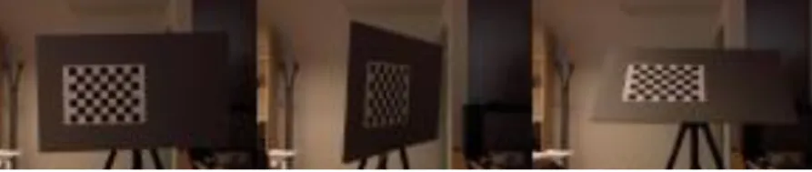
RGB-D cameras acquire in each frame one RGB image plus a depth image [16], which means in each frame is possible to obtain a colored point cloud of the scene. But at the process of association of each depth value to one pixel (or a set of pixels) of the RGB image, some pixels of objects can get depth values of the background or vice-versa [11]. So some calibration process needs to be done. One easy to use method is by tracking some moving spherical object on both RGB and depth images [45] for a few seconds and with their center point locations it is possible to calibrate both images. Other method is by using a chessboard pattern above some flat surface (Figure 1), like a table, so that the color camera’s pose is calculated from this pattern and the depth sensor’s pose is calculated using the table’s surface, where the chessboard pattern is [17]. Then by establishing the relation between both poses it is possible to align the color image with the depth image.

2.3 Registration

Registration is the process of alignment of multiple captures, of the same scene or object, with different viewpoints. The result can be an extended version of a 2D image or a 3D representation of the scene / object.

The use of registration can be found in weather forecasting, creation of super-resolution images [50], in medicine, by combining multiple scans to obtain more complete information about the patient [54] (monitoring tumor growth, treatment verification), in cartography (map updating), and in computer vision (3D representation)[57]. There are four main types of applications that require registration:

- Different viewpoints, to expand a 2D view (Figure 2) [26] or acquire a 3D mesh of the scene (Figure 3) [53].

- Different times, to study and evaluate the changes over time in the same scene (motion tracking, global land usage or treatment evolution).

- Different sensors (Figure 4), to achieve a more complex and detailed representation of the scene (in medicine the fusion of different types of scans of the same person).

- Scene to model registration, to localize the acquired image by comparing it to some model of the scene [39] (2D/3D virtual representation) (object tracking, map updating).

(22)

State of the Art

7

Figure 2: Registration of two 2D images to expand the view [40].

Figure 3: Registration of 3D point clouds to build a 3D model.

(23)

State of the Art

8

The process of registration is very dependent on the type of scene being targeted, the type of sensors used for each capture and the final expected result [25] [38]. But, for almost every case, this process follows four main steps:

- Feature Detection. Distinctive features of the image or capture like blobs, edges, contours, line intersections or corners are detected in order to find correspondences between the images to be align [11]. These features must be represented in a way so that transformations like scale and rotation does not affect the feature identifier [27], also known as descriptor or feature vector. Some of the most common algorithms used in feature detection are Canny and Sobel for edge detection, Harris and SUSAN for edge and corner detection, Shi & Tomasi and Level curve curvature for corner detection, FAST, Laplacian of Gaussian and Difference of Gaussians for corner and blob detection, MSER, PCBR and Gray-level blobs for blob detection [5].

- Feature Matching. After finding and identifying the features of a capture, the process of matching these features is the next step. The idea is to find identical features in both the new capture and the reference model (or reference capture). From brute-force descriptors matching and FLANN (Fast Library for Approximate Nearest Neighbors) to pattern recognition [33] there are many different approaches to solve this problem however they are very dependent on the type of scene and the available processing time (quality vs performance).

- Transformation Model Estimation. This step is the most time consuming of all, especially if the targeted scene has non-static or non-rigid objects. Most of the times (just not to say all the times) the feature matching process is not perfect, matching some features wrongly result in the impossibility of finding a transformation model that works for every single match. One way of solving this problem is by estimating recursively a model that works for a set of matches until the size of that set is larger enough (RANSAC [7]). The remaining matches are discarded (considered as outliers). Other approach is using ICP (Iterative Closest Point [30]), that in some implementations does not need an individual feature matching process [28], each feature is paired with its closest neighbor (of a different capture) and the transformation model is recursively estimated (using a hill climbing algorithm) so the distance between neighbors gets close to zero. The most common type of models are for rigid body transformations with 6 parameters (3 rotations and 3 translations), affine transformations [32] with 12 parameters (translation, scaling, homothety, similarity transformation, reflection, rotation, shear mapping, and compositions) or an elastic transformation approach [21] for non-rigid body objects.

(24)

State of the Art

9

- Final Corrections. The last step of registration is the transformation of the new capture, using the estimated transformation model, and appending or comparing the result with the reference model or capture. In some cases, corrections must be made, normally on the edges of the new capture, so the final result looks like the result of a single capture and not the joining of multiple captures [36].

2.4 3D Registration

For 3D model reconstruction, each capture needs to go throw a registration process. With each capture being represented as a point cloud, the registration process can be solved using point cloud registration algorithms. The most common methods for general registration of point clouds are Iterative Closest Point (ICP) [31] and its variants. There are some other methods, more object specific, which uses contour tracking [10] or a reference model [14] for the initial registration. Other method is the use of markers, placed over the object, so that the initial registration can be done by tracking and matching these markers [44].

Iterative Closest Point and some variants

This algorithm starts with two point clouds and recursively tries to estimate the transformation model by following these steps:

- Association of points from one point cloud to the other.

- Estimation of the transformation model that minimizes a cost function. - Transformation of the second point cloud using the estimated model. - If the result is not good enough iterate from the first step.

For the association of points the distance can be used only and the closest pair of points is chosen [13]. Alternatively, a descriptor matching approach can be used, with descriptors obtained using Normal Aligned Radial Feature (NARF [42]), Point Feature Histograms (PFH [41]) or Persistent Feature Histogram [40], algorithms that use geometric relations of the neighbor points to create a descriptor for a 3D point, invariant to scaling and rotation. For the descriptor matching method an a priori step must be considered to remove the ambiguity of similar descriptors in flat surfaces, normally by using the closest point [39] or by using a color based descriptor, if the color information is available [29]. After this step, in some cases, a sampling algorithm (RANSAC [7]) is used to filter some outliers or mismatches.

The most common cost functions are least squares [48], Woods [19], normalized correlation [24], correlation ratio [9], mutual information [54] and normalized mutual

(25)

State of the Art

10

information [12] [15]. The main problem of these cost functions are the local minima traps [8]. To avoid this problem, a low resolution version of the point clouds is used, with the resolution being iteratively increased until reaching the original version [20]. Another method that minimizes this problem is called Apodization of the Cost Function [19] that uses an estimation of the overlapping window of points in each point cloud to smooth the cost function, reducing local minima.

The two main variants of ICP are point-to-point and point-to-plane [31], where the main difference is the input of the cost function. Point-to-point methods only uses the squared distance of the two linked points of each point cloud to minimize the error and the point-to-plane uses the squared distance and the difference between the tangent point-to-planes of each point. The point-to-plane approach usually shows better results [23].

ICL and ICT

Iterative closest line (ICL) is similar to ICP but instead of matching points it matches lines. Hough transformation is an edge detection method used to extract lines on 2D images but it can be used in 3D point clouds (Figure 5) as well by projection [3]. ICL works great if the scene is rich in edges, like some city view with multiple buildings.

Iterative closest triangle patch (ICT) has the same principle of ICL but instead of searching for lines it uses sets of three points to form triangles [22]. For flat surfaces it uses bigger triangles, with far away points, and for curve surfaces it uses more and smaller triangles.

(26)

State of the Art

11

2.5 Non-Rigid Registration

Registration of non-rigid objects cannot be solved by using common registration geometrical transformation models [12] (like rotations, translations or affine transformations), because from one point cloud to the other, the existence of some internal non-linear transformations is a possibility. Depending on the amount of deformation between point clouds there are some models that can be used, like elastic model [55] [52] and viscous fluid model [1]. The elastic model uses a pair of forces, internal and external, to estimate small deformations. This forces are estimated by calculating the derivative of the similarity for all degrees of freedom [18], using a B-spline representation [49] or a distance map represented using an octree spline [48] to speed up the process. To solve this step, two classes of optimizers can be used, deterministic methods, that assumes exact knowledge of criterion, and stochastic methods [52], that uses an estimation of a cost function. The viscous fluid model uses multiple forces to estimate greater number of types of deformations, which can lead to higher chances of miss registrations when the two point clouds are distant from each other.

There are two main types of non-rigid registration methods, one of them is by using a cost function that minimizes both the rigid transformation and the internal deformation, and the other one consists on finding the best rigid transformation first and then calculating the best deformation to match [37]. The first method shows better results when the rigid transformation is small, which gives room for more complex deformations [14]. The second method is more robust for finding the rigid transformation, when the data sets are far away, but only works for small and localized deformations [14].

(27)

State of the Art

12

2.6 Parametric Model

Parametric model is a surface or shape representation constituted by a set of Non-uniform rational basis spline. NURBS (Figure 6) is a mathematical model used to generate and manipulate curves or surfaces. This manipulation of the surface is done by moving control points, and the movement of each control point will affect the entire surface, with the intensity being based on the distance between the surface point and the control point.

The initial surface of the parametric model can have a variety of shapes, and the choice of this initial shape will have a major impact on the quality and performance of the final fitting [6]. Some examples are the use of a superellipsoid (Figure 7) for the fitting of objects, or the use of a plane (Figure 8) for the fitting of a surface.

Figure 6: An example of a NURBS curve.

(28)

State of the Art

13

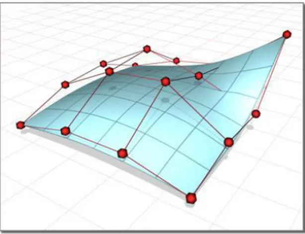
The fitting of the parametric model to the reference object or surface, is done by calculating the displacement vector of each control point, so that minimizes the displacement field between the parametric model surface and the reference surface [6]. The figures 9, 10, 11 and 12 are an example of the fitting process.

Figure 8: Example of surface fitting when using the plane as initial shape of the parametric model.

Figure 9: Reference object [6]. Figure 10: Initial shape of the parametric

(29)

State of the Art

14

The use of a parametric model for non-rigid registration can be a solution for the deformation correction. If it is possible to fit the parametric model to the point cloud with deformations, then the non-rigid alignment can be done by fitting this point cloud with deformations, now being represented as a parametric model, to the reference point cloud. This method can also be used to fill gaps occurring due to occlusions [56].

2.7 Conclusions

After this initial research, we can conclude that for rigid registration there are a great variety of methods and algorithms, each one with its improvements and drawbacks, with the success very dependent on the capture environment. For the non-rigid registration, the existing methods are dependent on a high quality and precision acquisition system, because noisy data have a stronger impact. In order to align point clouds with deformations, at least one point cloud needs to be a reference for the others. So if the reference point cloud have noisy data then all the point clouds with “good” data are going to be wrongly deformed.

Figure 11: Displacement field between the parametric model surface and the reference object surface [6].

Figure 12: Final shape of the parametric model after the fitting [6].

(30)

A 3D Reconstruction approach for RGB-D Images

15

Chapter 3

A 3D Reconstruction approach for

RGB-D Images

In this chapter a proposal will be described, step by step of the implementation to achieve our objectives, the 3D model reconstruction of rigid or non-rigid objects. Some examples of the results of the most important steps will be presented.

3.1 Captures and Point Clouds

The chosen sensor for the captures was the Microsoft Kinect over the Asus Xtion Pro Live mainly because of the online support, tutorials, forums, online community and the known compatibility with tools like PCL.

At this early stage the goal was to obtain color and depth images using the Microsoft Kinect sensor. For this purpose it was used the SDK “Kinect for Windows v2” for the communication with the sensor and obtaining the images. This tool is also used for the creation of point clouds resulting from the junction of the color information, depth and calibration parameters. These calibration parameters are obtained directly from the sensor and are constantly being updated. The capture rate (frame rate) can be set by the user, being limited only to the storage speed of each point cloud on the hard drive. Figure 13 shows a flowchart of the capture process.

(31)

16

3.2 Registration

The first approach used for a possible settlement of the main objective, 3D reconstruction of non-rigid objects, is the implementation of a variant of ICP with a cost function capable of obtaining the best rigid geometric transformation, without being influenced by possible deformations. The idea would be to use different weights for each point in the cost function, in such way that these weights would be the certainty of each point belonging to a rigid or non-rigid region of the point cloud.

This approach has been interrupted due to the difficulty of implementing the cost function with exact methods, so it was decided the use of approximate methods already implemented in PCL library [43]. With the PCL it is not possible to change the behavior of the cost function, so it was chosen a different approach. The methodology then consists of two main steps, first find the best rigid alignment and then adjust the non-rigid regions. For the rigid alignment, two different methods of coarse registration were implemented, one for scenes and other for objects. The reconstruction process is not fully automatic yet, it needs the manual setup of two threshold values: the noise reduction threshold and the smoothing threshold. These thresholds will be presented below. Figure 14 shows a flowchart of the reconstruction process.

Figure 13: Flowchart of one iteration of the capture process.

(32)

17 - Noise Reduction

Before starting with the process of registration, each point cloud is filtered with the objective of improving its quality and reliability about the position of each point. The algorithm used is simple, not time consuming and presents good results (Figure 15 and Figure 16). This method consists on filtering each point, of the point clouds, that have a lower density value of neighbors than the noise reduction threshold.

Figure 15: Example of a point cloud before the noise reduction algorithm.

Figure 16: The same point cloud of Figure 6 after the noise reduction algorithm.

(33)

18 - Scenes

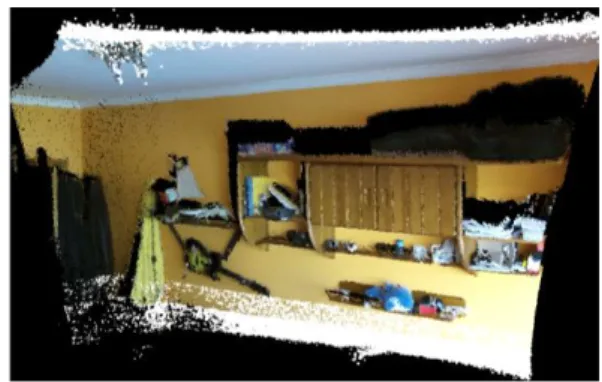
The first test cases were scenes (rooms captured from the inside) to be rich in corners and high-contrast regions in relation to color. With these specific attributes of scenes we concluded that it would be a good idea to use methods with feature points to use descriptors composed with color and curvature information, to determine an initial alignment required for the ICP algorithm. Unfortunately the results were not positive.

With this, we started to implement a different approach, consisting on several steps. Instead of feature points, the initial alignment was made up by comparison of the quality of the alignment after a limited number of iterations of a variant of ICP. This variant uses, as input of the cost function, the information of the curvature of each point, calculated with the geometric relations between neighbor’s points, along with the Euclidian distance, between each pair of closest points. At the first iterations it is used a smaller representation of the point cloud (sampled). The quality of the alignment is obtained iteratively and is compared between iterations, storing only the best. In each iteration is generated a different initial geometric transformation, that is applied to all points of the point cloud to be aligned in order to find a geometrical transformation that best approximates the actual transformation. After this, the final alignment is done by using the original version of ICP with a termination criteria of the type:

έ – ε < T, έ is the error of the previous iteration, ε is the error of the current iteration and T is a value close to zero (10−8_{was the value used).}

With this solution it is possible to align in most cases (Figure 17 and Figure 18), except in the parallel displacements between the sensor and surfaces with big flat regions (Figure 19). This is a problem for the correct alignment when using ICP, or its variants, due to the nature of these algorithms. When the point cloud to be aligned has a big flat region, the cost function will have a greater probability of getting stuck in a local minimum.

Figure 17: Two point clouds of the same scene, before the registration.

Figure 18: The same point clouds of Figure 8 after the registration.

(34)

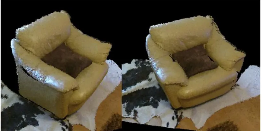
19 - Objects

For the registration of objects it was used a slightly different methodology. In this approach the initial alignment consists on a translation of one point cloud, so that the center of mass of both point clouds are at the same point, and a rotation obtained by the previous alignments:

𝑅 = 𝐿𝐸

Where R is the initial rotation for the current point cloud, L is the final rotation of the last aligned point cloud and E is the initial rotation of the last aligned point cloud. For the first iteration, R is initialized with the identity matrix.

After this step it was used the ICP variant with the curvature information. The results were very positive (Figure 20) for most of the objects.

Figure 19: Example of failed registration when the sensor is moving parallel to a surface with big flat regions.

Figure 20: Example of a successful alignment after the registration of 30 point clouds (captured at 10 fps).

(1) Figu re 20: Example of a successfu l alignment after the registratio n of 30 point clouds (captured at 10 fps).(1) Figu re 20: Example of a successfu l alignment

(35)

20

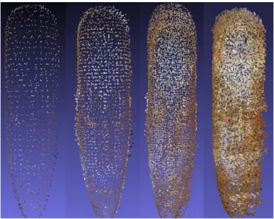
The small objects were having a problem with the density of the point clouds, in such way that in some cases the density of the noise was close to the density of the real data of the object. This way the noise was not being filtered after the noise reduction step (Figure 21 and Figure 22), because the algorithm uses the density value to remove the noise (described above).

To improve the quality of the final 3D models, reconstructed from small objects, we added a smoothing step between consecutive alignments. The smoothing algorithm consists in dividing the point cloud in small cubes and calculating the center point of each set of points, inside each cube. The dimensions of these cubes is calculated using the smoothing threshold that needs to be set manually, and works as a tradeoff between low density of accurate data or higher density of data with a percentage of noise (Figure 23).

Figure 21: Three views of 5 aligned point clouds of a small object.

Figure 22: Three views of 50 aligned point clouds of a small object.

(36)

21

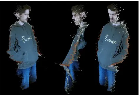
3.3 Non-rigid alignment

If there is some kind of movement or deformation in the objects during the captures, rigid registration of the various resulting point clouds is not enough. To solve this problem two different approaches have been implemented with the objective of correcting the regions with deformations. The first algorithm is simple and fast, but is a point-to-point approach so it can be vulnerable to some inconsistencies and discontinuities, the second method is based on the use of a parametric model but only works for small regions of the point cloud at each time.

Point-To-Point approach

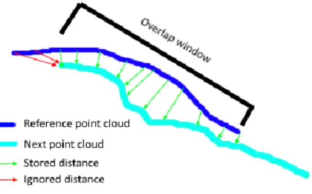
This method is applied after the rigid registration, described in the previous section, and consists in the following steps:

- Identification of the overlap window. In this stage the closest points from the reference point cloud to the next point cloud are calculated. During this step the smallest calculated distance for each point of the next point cloud is stored (Figure 24). For example, with points A and B points in the reference point cloud and point C in the next point cloud, if the closest point of A and B in the next point cloud is C, then the distance to be stored is the lower between 𝐴𝐶̅̅̅̅ and 𝐵𝐶̅̅̅̅. This way, the points that do not have a stored value for the distance are considered as outside of the overlap region.

- Identification of the region with deformation. Using the minimum distances calculated in the previous step, all points that have a distance greater than the mean density of the data on the reference will be considered as points belonging to the region with deformation (Figure 25).

(37)

22

- Alignment of the rigid region. In this step points of the next point cloud to be added to the reference point cloud are selected. These points are those in the overlap window but outside the region with deformation.

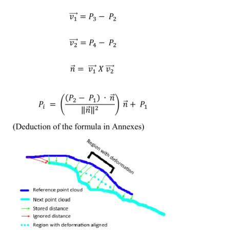
- Alignment of the region with deformation. For each point identified as belonging to the region with deformation, are calculated three points closer to that point in the reference point cloud. With these three points (𝑃₂, 𝑃3, 𝑃4) is calculated the equation of the plane, then is

calculated the equation of the line perpendicular to this plane passing through the initial point (𝑃₁). With this plane and this line is calculated the intersection point. This point of intersection (𝑃_𝑖) is then added to the reference point cloud (Figure 26).

𝑣1 ⃗⃗⃗⃗ = 𝑃3− 𝑃2 𝑣2 ⃗⃗⃗⃗ = 𝑃4− 𝑃2 𝑛⃗ = 𝑣⃗⃗⃗⃗ 𝑋 𝑣1 ⃗⃗⃗⃗ 2 𝑃𝑖 = ( (𝑃₂− 𝑃1) ∙ 𝑛⃗ ‖𝑛⃗ ‖2 ) 𝑛⃗ + 𝑃1

(Deduction of the formula in Annexes)

Figure 25: Illustration of the identification of the region with deformation step.

Figure 26: Illustration of the alignment of the region with deformation.

(4) (4) (4) (4) (2) (2) (2) (2) (3) (3) (3) (3) (5) Figu re 26: Illustratio n of the alignment of the region with deformati on.(5) Figu re 26: Illustratio n of the alignment

(38)

23

- Alignment of the region outside the overlap window. For each point, considered as belonging to the region outside the overlap window, the closest point in the reference point cloud is calculated. In the case that the angle between the vector formed by these two points and the normal vector at the closest point in the reference point cloud are near 90 degrees, then this point is added to the reference point cloud.

After all these steps is possible to align two point clouds with small deformations (Figure 27 and Figure 28).

Figure 27: Multiple views of the result of rigid registration between two point clouds with small deformations.

(39)

24 Parametric Model approach

A different approach was also explored, the use of a parametric model to rectify the discontinuities resulting from rigid registration of point clouds with deformations. The Figure 29 is the result of the rigid registration of point clouds obtained from patients. The region with higher discontinuities was at the belly (Figure 30, Figure 32). The Figure 31 is a drawing of this surface for a better understanding of the problem.

Figure 29: Result after rigid registration Figure 30: Selection of the region with discontinuities

Figure 31: Illustration of the discontinuities on the selection

(40)

25

After the selection of this region with discontinuities, it was used a parametric model to fit with this selection. The starting shape of the parametric model was a plane and the equation of the model is:

𝑋 = ∑ ∑ 𝐶𝑙𝑖 𝑚 𝑗=0 𝑙 𝑖=0 𝐶𝑚𝑗(1 − 𝑠)𝑙−𝑖𝑠𝑖(1 − 𝑡)𝑚−𝑗𝑡𝑗𝑃𝑖𝑗

The points at the surface of the model are represented as X, the control points are represented as P and the other members of the equation are representing the function responsible for the intensity distribution of displacement of each control point over the entire surface of the model.

The resulting parametric model, after the fitting with the region with discontinuities, will replace the selection (Figure 33), in the need of rectification, and after a simple smoothing the model no longer has discontinuities at that region (Figure 34).

Figure 33: Replacement of the selection with the parametric model

Figure 34: Final result after the smoothing

(6) Figu re 34: Final result after the smoothin g(6) Figu re 34: Final result after the smoothin g(6) Figu re 34: Final result after the smoothin g(6)

(41)

Validation and Results

26

Chapter 4

Validation and Results

During this chapter, the validation of the proposed methodology will be presented and some results will be discussed.

4.1 Validation with rigid objects

For the validation of our methodology it was used a high precision sensor as a ground truth. This sensor was the David laserscanner, which is composed by a normal RGB camera, a hand laser and a calibration background plane (Figure 35). This sensor uses a method called triangulation based laser range finder to capture the xyz coordinates of the objects [2]. In short words the method consists in projecting a laser ray, with the shape of a line, against the calibration background plane. By using the RGB camera to capture the image of the projected ray is possible to calculate the equation of the laser’s ray plane. When an object is placed between the calibration background plane and the RGB camera (Figure 36), the shape of the object can be obtained by using the equation of the laser’s ray plane and the image of the projected laser on the surface of the object.

(42)

27

The objects used for validation were of the type rigid, because the David laserscanner can only capture small rigid objects. Only the rigid registration methods were validated, when using this sensor as ground truth.

The validation process was done by comparison between the reconstruction of the 3D models of the objects in the Figure 37 and Figure 40, using the Microsoft Kinect with our framework (Figure 39 and Figure 42) and using the David laserscanner with David’s 3D reconstruction software (Figure 38 and Figure 41). Multiple configurations of the smooth threshold and noise reduction threshold were used for better understanding of its impact on the final result. As a comparison measure was used the mean of the Euclidian distances, between the 3D models of each object, after a manual alignment (results on Table 3).

Figure 36: Illustration of the use of the David laserscanner.

Figure 35: Two pictures of the components of the David laserscanner.

(43)

28

Figure 37: Rigid object used for validation.

Figure 38: 3D model reconstruction with David laserscanner.

Figure 39: 3D model reconstruction with Microsoft Kinect.

(44)

29

Figure 40: Rigid object used for validation.

Figure 41: 3D model reconstruction with David laserscanner.

Figure 42: 3D model reconstruction with Microsoft Kinect.

(45)

30 Table 3: Validation results of rigid objects.

First object (Figure 37) Smooth threshold value Noise reduction threshold value

Mean of the Euclidian distances (mm), using the direction from the David laserscanner model to the Microsoft Kinect model

Mean of the Euclidian distances (mm), using the direction from the Microsoft Kinect model to the David laserscanner model Mean of both distances (mm) 0.005 0.004 5 4 4.5 0.005 3 5 4 0.006 3 6 4.5 0.007 3 8 5.5 0.0005 0.005 3 5 4 0.0010 2 5 3.5 0.0050 3 5 4 0.0100 5 5 5

Second object (Figure 40) Smooth threshold value Noise reduction threshold value

Mean of the Euclidian distances (mm), using the direction from the David laserscanner model to the Microsoft Kinect model

Mean of the Euclidian distances (mm), using the direction from the Microsoft Kinect model to the David laserscanner model Mean of both distances (mm) 0.005 0.005 10 4 7 0.006 7 6 6.5 0.007 4 8 6 0.008 4 8 6 0.009 4 10 7 0.0001 0.007 3 7 5 0.0005 3 7 5 0.0010 3 7 5 0.0030 4 8 6 0.0050 4 8 6

(46)

31

The variation of results were as expected, when using different values for the smooth threshold and the noise reduction threshold.

The value used for the noise reduction threshold, have greater impact on the mean of the Euclidean distances, when using the direction from the Microsoft Kinect model to the David laserscanner model. This is because every single point of the Microsoft Kinect model will be used for the calculation of the distances, and by increasing the value of the noise reduction threshold, the number of noisy points used for the calculations will increase as well, leading to worst results as expected. On the other hand, if the value of this threshold is lower than the density of the “good” data, then the model will start losing detail. This loss of detail can be detected when the value of the mean of the Euclidean distances, when using the direction from the David laserscanner model to the Microsoft Kinect model, increases. When using this direction for the calculation of the mean of the Euclidean distances, the increase of the noise reduction threshold value does not change the result, because only the closest points of the Microsoft Kinect model will be used for the calculation of the Euclidean distances, this way the increase of noisy data does not change the results when using this direction.

The smooth threshold is used to increase the accuracy of the data on the surface of the 3D model, by decreasing the density of the data. The increase of the smooth threshold value will increase the accuracy of the data, but after a certain value the model will start losing detail. This loss of detail can be detected when the mean of the Euclidean distances of both directions increases.

4.2 Validation with non-rigid objects

The validation by comparison with a ground truth model, of the point-to-point approach, was not possible. The results after the use of this approach to align two point clouds with deformations, are visually positives. The Figure 43 is the result after the rigid registration, where it can be seen two not aligned surfaces at the face region. This deformation between the point clouds is the result of the forward movement of the head. The Figure 44 is the result after the non-rigid registration, using the point-to-point approach. At the face region, only one surface can be seen which represents a good non-rigid alignment of the point clouds.

(47)

32

Figure 43: Rigid registration of two point clouds with deformations.

(48)

33

For the validation of the parametric model approach, the high precision sensor 3dMD (Figure 45) was used to obtain the models for comparison. The validation consists in comparing the rigid reconstruction, of three patients captured with Microsoft Kinect (Figures 46, 47 and 48), with the models obtained from the 3dMD sensor, and then verifying the improvements of using the parametric model approach by comparing its results with the models obtained from the 3dMD sensor (Table 4).

Figure 45: 3dMD sensor

Figure 46: 3D models of patient A, the rigid reconstruction on the left, the result of the parametric model approach on the middle and the reconstruction from the 3dMD sensor on the right

(49)

34

Figure 47: 3D models of patient B, the rigid reconstruction on the left, the result of the parametric model approach on the middle and the reconstruction from the 3dMD sensor on the right

Figure 48: 3D models of patient C, the rigid reconstruction on the left, the result of the parametric model approach on the middle and the reconstruction from the 3dMD sensor on the right

(50)

35 Table 4: Validation results of non-rigid objects Patients Mean of the Euclidian

distances (mm), using the direction from the 3dMD model to the Microsoft Kinect model

Mean of the Euclidian distances (mm), using the direction from the Microsoft Kinect model to the 3dMD model Mean of both distances (mm) A (after rigid registration) 8 11 9.5 A (after non-rigid registration) 7 7 7 B (after rigid registration) 7 7 7 B (after non-rigid registration) 7 5 6 C (after rigid registration) 7 9 8 C (after non-rigid registration) 8 8 8

The results presented on table 4 are very positive, considering that only a small selection of each model was non-rigidly improved. These improvements are more visible when calculating the mean of the Euclidian distances using the direction from the Microsoft Kinect model to the 3dMD model, because of the increase on the accuracy and the decrease on the density of the data.

(51)

Conclusions and Future Work

36

Chapter 5

Conclusions and Future Work

5.1 Conclusions

3D reconstruction is a complex process, normally associated to expensive sensors and experienced staff. It cannot be found a single low-cost and practical system in the market, with sensor, software and the purpose of general 3D reconstruction of rigid and non-rigid objects.

A study of the most common registration algorithms was presented in this document. The main conclusions gathered are that each different type of approach or algorithm to align point clouds are very dependent of the target, object or scene, and to achieve optimal results with different types of targets is really hard to make the process fully automatic.

Our framework is not ready to be used by unexperienced people yet, but it can be seen as a small step forward towards the general 3D reconstruction of rigid and non-rigid objects. It is composed by a set of operations that allows the user to capture a scene or an object, with the Microsoft Kinect sensor in his hands, and after the manual setup of some thresholds, the 3D model is generated.

Two non-rigid registration methodologies were implemented, the point-to-point approach for automatic and object independent registration, but a lesser robustness to discontinuities and inconsistency, and the parametric model approach, that because of the way is manipulated makes it more robust to discontinuities, inconsistency and occlusions. This last approach, with the parametric model, showed good results even when only using for a small region of the 3D model.

(52)

Conclusions and Future Work

37

5.2 Future Work

For future work the most important improvements could be:

- The use of ICT for the registration of point clouds from scenes, for being more robust to big flat regions.

- The extension of the parametric model approach to the entire 3D model. There are two possible paths, the use of multiple parametric models each one with different characteristics to match each region of the 3D model, or the use of a single parametric model with sufficient deformation freedom to match the entire 3D model.

- The automatic setup of thresholds for target independent 3D reconstruction and better usability by unexperienced people.

(53)

References

38

References

[1]: Emiliano D’Agostino, Frederik Maes, Dirk Vandermeulen, Paul Suetens. A viscous fluid model for multimodal non-rigid image registration using mutual information. Faculties of Medicine and Engineering, Medical Image Computing (Radiology-ESAT/PSI), Katholieke Universiteit Leuven, University Hospital Gasthuisberg, Belgium. 2003.

[2]: E. Alby, E. Smigiel, P.Assali, P.Grussenmeyer, I.Kauffmann-Smigiel. Low Cost Solutions For Dense Point Clouds Of Small Objects: Photomodeler Scanner Vs. David Laserscanner. Photogrammetry and Geomatics Group, Graduate School of Science and Technology (INSA), Etude des Civilisations de l'Antiquité, CNRS - Université de Strasbourg, France. 2009.

[3]: Majd Alshawa. Icl: Iterative closest line A novel point cloud registration algorithm based on linear features. 2007.

[4]: Simon R. Arridge and Martin Schweiger. Direct calculation of the moments of the distribution of photon time of flight in tissue with a finite-element method. Department of Computer Science, Department of Medical Physics and Bioengineering, University College London. 1994.

[5]: Anna Babaryka. Recognition from collections of local features. Master of Science Thesis Stockholm, Sweden. 2012.

[6]: Eric Bardinet, Laurent D. Cohen, Nicholas Ayache. A Parametric Deformable Model to Fit Unstructured 3D Data. 2006.

[7]: Chu-Song Chen, Yi-Ping Hung, Jen-Bo Cheng. RANSAC-Based DARCES: A New Approach to Fast Automatic Registration of Partially Overlapping Range Images. IEEE Computer Society. 1999.

[8]: Dmitry Chetverikov, Dmitry Stepanov. Robust Euclidean alignment of 3D point sets: the Trimmed Iterative Closest Point algorithm. Computer and Automation Research Institute Budapest. 2005.

[9]: Jamie Cook, Vinod Chandran, Sridha Sridharan and Clinton Fookes. Face Recognition From 3d Data Using Iterative Closest Point Algorithm And Gaussian Mixture Models. Image and Video Research Lab Queensland University of Technology. 2004.

[10]: Elisa García Corisco. Registration of Ultrasound Medical Images. 2014.

[11]: Pedro Miguel Ferro da Costa. Kinect Based System for Breast 3D Reconstruction. Faculdade de Engenharia da Universidade do Porto. 2014.

(54)

References

39

[12]: W. R. Crum, T. Hartkens and D. L. G. Hill. Non-rigid image registration: theory and practice. Division of Imaging Sciences, The Guy’s, King’s and St. Thomas’ School of Medicine, UK. 2004.

[13]: Andrew W. Fitzgibbon. Robust registration of 2D and 3D point sets. Department of Engineering Science, University of Oxford, UK. 2003.

[14]: Thomas Funkhouser and Shi-Min Hu. As-Conformal-As Possible Surface Registration. Eurographics Symposium on Geometry Processing. 2014.

[15]: T. Hartkens, D. Rueckert, J.A. Schnabel, D.J. Hawkes, D.L.G. Hill. VTK CISG Registration Toolkit An open source software package for affine and non-rigid registration of single- and multimodal 3D images. Computational Imaging Sciences Group, King’s College London, London, UK. 2002.

[16]: Peter Henry, Michael Krainin, Evan Herbst, Xiaofeng Ren, Dieter Fox. RGB-D Mapping: Using Depth Cameras for Dense 3D Modeling of Indoor Environments. University of Washington, Department of Computer Science & Engineering. 2010.

[17]: Daniel Herrera, Juho Kannala, and Janne Heikkila. Joint depth and color camera calibration with distortion correction. Center for Machine Vision Research, University of Oulu, Finland. 2012.

[18]: Alfonso A. Isola, Michael Grass, Wiro J. Niessen. Fully automatic non-rigid registration-based local motion estimation for motion-corrected iterative cardiac CT reconstruction. Philips Technologie GmbH Forschungslaboratorien, Germany and Biomedical Imaging Group Rotterdam, Erasmus MC, University Medical Center Rotterdam, The Netherlands. 2010.

[19]: Mark Jenkinson, Peter Bannister, Michael Brady, Stephen Smith. Improved Optimization for the Robust and Accurate Linear Registration and Motion Correction of Brain Images. Oxford Centre for Functional Magnetic Resonance Imaging of the Brain, John Radcliffe Hospital, Headington, and Medical Vision Laboratory, Department of Engineering Science, University of Oxford, Parks Road, Oxford, United Kingdom. 2001.

[20]: Timothée Jost and Heinz Hügli. A Multi-Resolution ICP with Heuristic Closest Point Search for Fast and Robust 3D Registration of Range Images. Institute of Microtechnology, University of Neuchâtel, Switzerland. 2003.

[21]: F Lamare, M J Ledesma Carbayo, T Cresson, G Kontaxakis, A Santos, C Cheze Le Rest, A J Reader and D Visvikis. List-mode-based reconstruction for respiratory motion correction in PET using non-rigid body transformations. School of Chemical Engineering & Analytical Science, The University of Manchester, Manchester, UK. 2007.

[22]: Qingde Li and J. G. Griffiths. Iterative Closest Geometric Objects Registration. Department of computer Science University of Hull, UK. 2000.

[23]: Kok-Lim Low. Linear Least-Squares Optimization for Point-to-Plane ICP Surface Registration. Department of Computer Science University of North Carolina at Chapel Hill. 2004.

(55)

References

40

[24]: Bruce D. Lucas, Takeo Kanade. An Iterative Image Registration Technique with an Application to Stereo Vision. Computer Science Department, Carnegie-Mellon University, Pittsburgh, Pennsylvania. 1981.

[25]: Ameesh Makadia, Alexander Patterson, Kostas Daniilidis. Fully Automatic Registration of 3D Point Clouds. University of Pennsylvania. 2006.

[26]: Jean François Mangin, Vincent Frouin, Isabelle Bloch, Bernard Bendriem and Jaime Lopez Krahe. Fast Nonsupervised 3-D Registration of PET and MR Images of the Brain. Service Hospitalier Frédéric Joliot, CEA, Orsay, France. 1994.

[27]: B. S. Manjunath, C. Shekhar and R. Chellappa. A New Approach to Image Feature Detection with Applications. Department of Electrical and Computer Engineering, University of California, Santa Barbara, and Center for Automation Research, University of Maryland, U.S.A. 1996.

[28]: Jorge L. Martínez, Javier González, Jesús Morales, Anthony Mandow and Alfonso J. García-Cerezo. Mobile Robot Motion Estimation by 2D Scan Matching with Genetic and Iterative Closest Point Algorithms. Department of System Engineering and Automation University of Málaga. 2006.

[29]: Hao Men and Kishore Pochiraju. Hue-assisted automatic registration of color point clouds. Department of Mechanical Engineering, Stevens Institute of Technology, USA. 2014.

[30]: Javier Minguez, Luis Montesano, and Florent Lamiraux. Metric-Based Iterative Closest Point Scan Matching for Sensor Displacement Estimation. IEEE TRANSACTIONS ON ROBOTICS. 2006.

[31]: Niloy J. Mitra, Natasha Gelfand, Helmut Pottmann, and Leonidas Guibas. Registration of Point Cloud Data from a Geometric Optimization Perspective. Computer Graphics Laboratory, Stanford University, Geometric Modeling and Industrial Geometry, Vienna University of Technology. 2004.

[32]: Feroz Morab, Sadiya Thazeen, Mohamed Najmus Saqhib and Seema Morab. Image Registration using Affine Transforms based on Cross-Correlation. Department of Electronics and Communication Engineering, VTU, Bangalore, India. Amity University, Noida, India. 2014.

[33]: David M. Mount, Nathan S. Netanyahu, Jacqueline Le Moigne. Efficient algorithms for robust feature matching. Department of Computer Science and Institute for Advanced Computer Studies, University of Maryland, USA. 1999.

[34]: Hélder P. Oliveira, Jaime S. Cardoso, André T. Magalhães & Maria J. Cardoso. A 3D low-cost solution for the aesthetic evaluation of breast cancer conservative treatment. Computer Methods in Biomechanics and Biomedical Engineering: Imaging & Visualization, 2:2, 90-106, DOI: 10.1080/21681163.2013.858403. 2014.

[35]: Hélder P. Oliveira, Jaime S. Cardoso, André Magalhães and Maria J. Cardoso. Methods for the Aesthetic Evaluation of Breast Cancer Conservation Treatment: A Technological Review. INESC TEC and Faculdade de Engenharia, Faculdade de Medicina,