http://dx.doi.org/10.12988/ams.2014.4143
Multiple Solutions of Mixed Variable Optimization
by Multistart Hooke and Jeeves Filter Method
M. Fernanda P. Costa
Department of Mathematics and Applications, University of Minho, Portugal Centre of Mathematics, University of Minho
Florbela P. Fernandes
Department of Mathematics, Polytechnic Institute of Bragan¸ca, Portugal Centre of Mathematics, University of Minho
Edite M.G.P. Fernandes and Ana Maria A.C. Rocha
Algoritmi Research Centre, University of Minho, Portugal
Copyright c 2014 M. Fernanda P. Costa et al. This is an open access article dis-tributed under the Creative Commons Attribution License, which permits unrestricted use, distribution, and reproduction in any medium, provided the original work is properly cited.
Abstract
Mathematics Subject Classification: 90C11; 90C26; 90C56
Keywords: Multistart, mixed variables, Hooke and Jeeves, filter method
1
Introduction
This paper presents a multistart method based on a derivative-free local search procedure, the Hooke and Jeeves method [8], to locate multiple solutions of nonlinear constrained mixed variable optimization (MVO) problems. This type of problem contains both continuous and integer decision variables and we use the following mathematical form
min f(x, y)
subject to gi(x, y)≤0, i= 1, . . . , m
hj(x, y) = 0, j = 1, . . . , p
lx ≤x≤ux, ly ≤y≤uy
(1)
where x, lx, ux ∈ Rnx, y, ly, uy ∈ Zny (in particular y ∈ {0,1}ny), nx is the
number of continuous variables, ny is the number of integer variables, lx and
ly are the vectors of the lower bounds for the continuous and discrete variables
respectively, andux anduy are the vectors of the corresponding upper bounds.
We will use n to represent the total number of variables of the problem. We do not assume that the functions f, gi, i = 1, . . . , m and hj, j = 1, . . . , p are
convex and thus many global and local (non-global) solutions may exist. It is not an easy task to compute just one solution of the MVO problem, to compute multiple solutions (global and local) in an MVO context is therefore one of the most complex optimization problems.
The most common deterministic approaches to compute a global solution of MVO problems are branch and bound techniques, outer approximation, general Benders decomposition and extended cutting plane methods. The main advantage of these approaches is that they may guarantee to find the global optimum, although they also require large amounts of computational time. In general, the complexity rises exponentially with the dimension of the problem.
Recent derivative-free methods for locating a local minimizer of MVO prob-lems are presented in [1, 12]. In the first paper, the generalized pattern search algorithm for linearly constrained (continuous) optimization was extended to mixed variable problems and the constraints are treated by the extreme bar-rier approach. In the second paper, a minimization of a penalty function dis-tributed along all the variables is performed. Continuous and discrete search procedures, as well as a penalty parameter updating rule are the most relevant issues of the therein presented method.
In this paper, we address the issue of locating multiple solutions of MVO problems by using a multistart paradigm and extending the Hooke and Jeeves (HJ) method to inequality and equality constrained problems and integer vari-ables. The HJ method, developed for unconstrained optimization, uses ex-ploratory and pattern moves to locally search for a point that improves the objective function value relative to a central point of the search [8, 9]. When the variables of the problem must satisfy a set of bound or/and inequality and equality constraints, the basic HJ algorithm should be extended to ensure that only feasible points are considered as potential solutions. The extension herein presented uses a reformulation of problem (1) as a bound constrained bi-objective optimization problem and includes a filter methodology [2, 3, 5] to assess objective and constraint violation functions to promote convergence to feasible and optimal solutions. Furthermore, discrete values for the inte-ger variables are ensured by using a specific pattern of points spread over the search space. The multistart HJ filter method presented in this study is an extension of the work proposed in [4], in the sense that multiple solutions have now to be located in a single run of the algorithm targeting both global and lo-cal minimizers. A multistart method is a suitable stochastic strategy to locate multiple solutions. Since some solutions may be computed more than once, the concept of region of attraction is integrated into the algorithm to avoid repeated convergence to previously computed solutions.
2
Multistart method
This section presents the main ideas of a multistart method that uses the concept of region of attraction to avoid repeated convergence to previously computed solutions. This is the most popular stochastic method when mul-tiple solutions are required. To compute mulmul-tiple solutions, the simplest idea is to repeatedly call/invoke a local search procedure starting each time from a different randomly selected point, so that hopefully different optimal solutions will be found. However, the same solutions may be computed over and over again. Convergence to previously computed solutions can be avoided by imple-menting a clustering technique which aims to define prohibited regions based on the closeness to the previously computed solutions [16, 17, 18]. Each time a point is randomly selected from these prohibited regions, it will be discarded since the implementation of the local search procedure will eventually produce one of the previously computed solutions. This way the number of calls to the local search procedure is reduced. The ultimate goal of a multistart algorithm is to invoke the local search procedure as many times as the number of optimal solutions of problem (1).
Our implementation of a multistart method for MVO problems defines the randomly selected starting points as follows:
xi = (lx)i+λ((ux)i−(lx)i) for i= 1, . . . , nx
yj = (ly)j +τj for j = 1, . . . , ny
(2)
where the notation (lx)i stands for the component i of the vector lx, λ is
a random value uniformly distributed in [0,1] and τj is a number randomly
selected from the set {0,1, . . . ,((uy)j −(ly)j)}. In what follows, we will use
the following notation: X = (x, y)T to represent the vector of the n variables,
L= (lx, ly)T and U = (ux, uy)T to represent the vectors of the bounds on the
variables.
The region of attraction of a minimizer, X∗
= (x∗ , y∗
)T, associated with a
local search procedure L, is defined as:
A ≡ {X ∈[L, U] :L(X) =X∗
}, (3)
where L(X) produces the minimizer X∗
after invoking the local search pro-cedure L starting at the point X. This means that if a point X is randomly selected from the set [L, U] and belongs to the region of attraction A of the minimizerX∗
, then this minimizer would be obtained whenLis invoked start-ing from that X. Thus, the main idea is to invoke the local search procedure only when the randomly selected point does not belong to any of the regions of attraction of already computed minimizers or, equivalently, to the union of those regions of attraction, since they do not overlap. However, it is not an easy task to compute the region of attraction A of a minimizer X∗
alternative process consists of estimating the probability, p, that a sampled point will not belong to the union of the regions of attraction of the previously computed minimizers. This is estimated by the probability that the sampled point will not belong to the region of attraction of the nearest toX minimizer, herein denoted by X∗
o (where o is used to denote the index of this particular
minimizer), i.e.,
p=P rob[X /∈ ∪s
i=1Ai] = s
Y
i=1
P rob[X /∈Ai]≈P rob[X /∈Ao]
wheresis the number of the already computed minimizers andAo is the region
of attraction of the minimizer X∗
o (see details in [18]). In practice, the value
of p is approximated by P rob[X /∈ B(X∗
o, Ro)], which is the probability that
the sampled point does not belong to the sphere centered at the minimizerX∗
o
with radius Ro. For any i, letRi represent the maximum attractive radius of
the minimizer X∗
i:
Ri = max j
n X
(j)
i −X
∗ i o , (4)
where Xi(j) is one of the sampled points that converged to the minimizer X∗
i
after invoking the local search procedure. Given X, let di = kX −Xi∗k be
the distance between the point X and the minimizer X∗
i. If di < Ri then
the point X is likely to be inside the region of attraction of X∗
i and the local
search procedure ought not to be invoked since the probability of converging to the minimizerX∗
i is high. However, if the direction fromX toX
∗
i is ascent
then X is likely to be outside the region of attraction of X∗
i and the local
search procedure ought to be invoked, starting fromX, since a new minimizer could be detected with high probability [18]. Thus, the estimated value of the probability thatX /∈Ai is
• 1, if di
Ri ≥1,
• 1, if di
Ri <1 but the direction fromX to X ∗
i is ascent,
• 0< ̺(X, X∗
i)Φ
di
Ri, ri
<1, if di
Ri <1 and the direction from X toX ∗
i is
descent,
where̺is a function that depends on the directional derivative off along the direction from X to X∗
i, ri is the number of times the minimizer Xi∗ might
have been recovered thus far, and Φ is a function that:
• tends to 0 as di
Ri approaches 0,
• tends to 1 as di
Ri approaches 1,
• tends to 0 as ri increases.
Here, we use the function Φ proposed in [18] for 0< di
Ri <1,
Φ
di
Ri
, ri
= di
Ri
exp −ri2
di
Ri
−1
and compute ̺(X, X∗
i) using forward differences to estimate de gradient of f
atX, δf(X),
̺(X, X∗
i) = 1 +
(X∗
i −X)Tδf(X)
kX∗
i −Xkkδf(X)k
.
We consider the direction fromX toX∗
i ascent if (X
∗
i −X)Tδf(X)> 0.
Algo-rithm 1 displays the main steps of the multistart algoAlgo-rithm. The set ∆∗
, empty at the beginning of the iterative process, contains the computed minimizers that are different from the previous ones. To check if a computed minimizer,
X∗
, has been previously identified the following proximity conditions must hold
|f(X∗
)−f(X∗
l)| ≤γ
∗
and kx∗
−x∗
lk ≤γ
∗
and ky∗
−y∗
lk= 0 (5)
for anyl in the indices set of previously identified minimizers {1, . . . , s}, and a small γ∗
> 0. Although this type of methods is simple, they would not be effective if a bad stopping rule is used. The main goal of a stopping rule is to make the algorithm to stop when all minimizers have been located with cer-tainty. Further, it should not require a large number of calls to the local search procedure to decide that all minimizers have been found. A simple stopping rule, adopted from [10], uses an estimate of the fraction of uncovered space,
P(s) = st((st−+1)1), where s gives the number of (different) computed minimizers and t represents the number of times the local search procedure has been in-voked. The multistart algorithm then stops if P(s) ≤ ǫ, for a small ǫ > 0. However, if this condition is not satisfied the algorithm is allowed to run for
Kmax iterations.
The next section addresses the issue related with the local search proce-dure,L. It is a derivative-free pattern search type method that is prepared to handle inequality and equality constraints by means of a filter methodology [2, 3, 5, 7]. The method extends the Hooke and Jeeves approach, as outlined in [8, 9], for solving a mixed integer constrained optimization problem. The herein presented study is an extension of the work proposed in [4], in the sense that multiple optima of problems like (1) are required rather than just a global optimum. Two crucial tasks are to be carried out: one is related with the defi-nition of the pattern in the HJ search procedure to take care of continuous and discrete variables simultaneously, and the other uses the filter methodology to handle the inequality and equality constraints. In what follows this extension will be called ‘mixed-HJ-filter’.
3
The ‘mixed-HJ-filter’ method
mini-Algorithm 1Multistart algorithm
Require: L,U,ǫ >0,Kmax, set ∆∗ =∅,s= 1, t= 1, k= 0; 1: Randomly generate X∈[L, U] using (2);
2: Compute X∗
1 =L(X),R1 =kX−X1∗k, set r1 = 1, ∆∗ = ∆∗∪X1∗; 3: repeat
4: Randomly generateX ∈[L, U] using (2);
5: Seto= arg minj=1,...,sdj ≡ kX−Xj∗k;
6: if do< Ro then
7: if the direction fromX toX∗
o is ascent then
8: Setp= 1;
9: else
10: Compute p=̺(X, X∗
o)Φ
do
Ro, ro
;
11: end if 12: else
13: Set p= 1;
14: end if
15: if rand(0,1)< pthen 16: Compute X∗
=L(X), set t=t+ 1;
17: if X∗
/
∈∆∗
then 18: Sets=s+ 1,X∗
s =X∗,rs= 1, ∆∗= ∆∗∪Xs∗, computeRs=kX−Xs∗k;
19: else
20: (X∗
=X∗
l ∈∆
∗
) UpdateRl= max{Rl,kX−Xl∗k},rl =rl+ 1;
21: end if 22: else
23: Update Ro= max{Ro,kX−Xo∗k},ro=ro+ 1;
24: end if
25: Setk=k+ 1;
26: until s(s+ 1)/((t(t−1))≤ǫork≥Kmax
mizer of the problem (1). Using a filter methodology [5], the basic idea is to reformulate (1) as a bi-objective optimization problem
min [f(x, y), θ(x, y)]
subject to lx ≤x≤ux, ly ≤y≤uy
(6)
whereθ(x, y) =kg(x, y)+k2
2+kh(x, y)k22 is the nonnegative constraint violation function and v+ = max{0, v}. The filter technique incorporates the concept of nondominance, borrowed from the field of multi-objective optimization, to build a filter set that is able to accept trial approximations if they improve the constraint violation or the objective function value. A filter F is a finite set of points (x, y), corresponding to pairs (θ(x, y), f(x, y)), none of which is dominated by any of the others. A point (x, y) is said to dominate a point (x′
, y′
) if and only ifθ(x, y)≤θ(x′ , y′
) andf(x, y)≤f(x′ , y′
).
the remaining part of this section. At the beginning of the iterative process, the filter is initialized toF = {(θ, f) :θ ≥ θmax}, where θmax >0 is an upper bound on the acceptable constraint violation.
3.1
Exploratory moves
Based on the current point (x, y), the search begins with a central point, set as (¯x,y¯) = (x, y), and defines a sequence of trial approximations along the unit coordinate vectorsei ∈Rn with a fixed step sizeαx∈(0,1]:
x+ = ¯x±αxDei, i= 1, . . . , nx, and y+ = ¯y±ei, i=nx+ 1, . . . , n, (7)
where D ∈Rnx×nx is a weighting diagonal matrix. The search for acceptable
trial points follows the rules:
• when searching along each ei to find a trial point that is acceptable by
the filter, the positive direction is tried first;
• each time a point (x+, y+) falls outside [L, U] the point is projected onto the search space [L, U];
• if the trial point improves over (¯x,y¯), reducingθorf by a certain amount, i.e., if one of the conditions
θ(x+, y+)<(1−γ
θ) θ(¯x,y¯) or f(x+, y+)≤(1−γf) f(¯x,y¯) (8)
holds, for fixed constants γθ, γf ∈(0,1), and is acceptable by the filter,
(x+, y+) is accepted and replaces (¯x,y¯);
• the search goes on along the remaining unit coordinate directions, as described above;
• if, on the other hand, the trial approximation (x+, y+) is dominated by the current filter, the search for a trial point is repeated, according to (7), but along the negative direction, before passing to the next unit coordinate direction.
We also note that whenever a point is acceptable, the point is added to the filterF, and all dominated points are removed from the filter.
When the search along thencoordinate vectors terminates, the most nearly feasible point (it may be a feasible one) among the accepted trial points is selected. Let that point be denoted by (xinf, yinf). If (xinf, yinf) 6= (x, y),
the search is termed successful and the vector (xinf, yinf)−(x, y) defines a
promising direction, known as pattern direction; otherwise the search is called unsuccessful, and a restoration phase is invoked.
3.2
Pattern moves
When a successful search occurs, a move along the pattern direction is carried out. The search along the n unit coordinate vectors, using (7) and the above described rules, is conducted using (xinf, yinf) + ((xinf, yinf)−(x, y)) as the
central point. At the end, the most nearly feasible point among the generated trial points is selected. When a new acceptable (xinf, yinf) is found then it is
accepted as the new iterate, replaces (¯x,y¯), and the pattern move is repeated.
3.3
Restoration phase
When it is not possible to find a non-dominated trial point, a restoration phase is invoked. In this phase, the most nearly feasible point in the filter, (xinfF , y
inf
F ), is recuperated and the search along the n coordinate vectors, as
previously described and using (7), is repeated but with (xinfF , y
inf
F ) as the
central point. When a non-dominated trial point is found, it becomes the central point for the next iteration. Otherwise, the iteration is unsuccessful, the search returns back to the current (¯x,y¯), the step size αx is reduced, and
a new search consisting of exploratory moves and pattern moves is repeated taking (¯x,y¯) as the central point.
3.4
Termination rule
Whenαx is reduced within an unsuccessful iteration, it may fall below a
suffi-ciently small positive tolerance,αmin. This is an indication that the first-order convergence has been attained [9] and the ‘mixed-HJ-filter’ algorithm may terminate.
4
Numerical Results
This section aims to analyze the performance of the presented multistart method based on the ‘mixed-HJ-filter’ algorithm (for simplicity, henceforth denoted by ‘MS+m-HJ-f’) when computing multiple solutions of MVO prob-lems. Seven MVO problems where selected from the literature [6, 7, 13]. The parameters of the multistart and ‘mixed-HJ-filter’ algorithms are set after an empirical study as follows: Kmax = 20, γ∗ = 0.005, ǫ = 0.1, γθ = γf = 10−8,
αmin = 10−4 and θmax = 102max{1, θ(¯x,y¯)}. Each problem was solved 30 independent times.
Problem 4.1 (Example 1 in [13]) with 2 known solutions (1 global and 1 local)
min −x−y
subject to xy−4≤0,
0≤x≤4, y∈ {0, . . . ,6}
The proposed ‘MS+m-HJ-f’ algorithm found two solutions. The global solution was found in all the 30 runs and the local in 24. The best global function value -6.666657 (with a constraint violation of 0.000000e+00) and minimizer (6.6665758e-01, 6) was produced by the ‘mixed-HJ-filter’ algorithm, in one of the 15 local ‘mixed-HJ-filter’ calls of run 28, after 0.861 seconds (sec), 604 function evaluations (feval) and 44 iterations (iter). On the other hand, the best value for the local solution, -5.000000 (with a constraint violation of 0.000000e+00) was attained at the point (4.000000e+00, 1) in one of the 18 local calls of run 20, after 1.273 sec, 369 feval and 31 iter.
Problem 4.2 (Example 11 in [13]) with 2 known solutions (1 global and 1 local)
min 35x0.6 1 + 35x
0.6 2
subject to 600x1−50y−x1y+ 5000 = 0
600x2+ 50y−15000 = 0
0≤x1≤34,0≤x2≤17, y∈ {100, . . . ,300}
When solving this problem, our algorithm found two optimal solutions, one global and one local. The global was located in all runs and the local only in two out of the 30 runs. (In the other runs, the algorithm terminated with a solution that is far away from the expected optimal value.) The best value 189.2946 (with a constraint violation of 0.000000e+00) for the global minimum was reached in one of the 5 local calls of the 11th run, after 4.532 sec, 683 feval and 28 iter of the ‘mixed-HJ-filter’ algorithm. The located minimizer was (0.000000e+00, 1.666417e+01, 100). On the other hand, the best value for the local solution 291.7167 (with a violation of 4.551885e-11) was found during one call of the local procedure (out of 15) of the run 16, after 1771 feval, 66 iter and 7.793 sec. The attained minimizer was (1.544511e+01, 6.831081e+00, 218).
Problem 4.3 (Example 21 in [13]) with 2 known solutions (1 global and 1 local)
min x0.6
1 +y
0.6
1 +y
0.4
2 −4y2+ 2x2+ 5y3−y4
subject to x1+ 2x2−4≤0
y1+y3−4≤0
y2+y4−6≤0
−3x1+y1−3x2= 0
−2y1+y2−2y3= 0
4x2−y4= 0
Two optimal solutions, one global and one local, were found in this case. The global was located in all runs and the local in 22 out of 30 runs. With a constraint violation of 0.000000e+00, one of the 21 local calls of run 13 reached the best objective function value for the global solution. To reach (1.6663651e-01, 4.999978e-01, 2, 4, 0, 2) with the optimal value of -13.40195, the local ‘mixed-HJ-filter’ required 6042 feval, 93 iter and 54.012 sec. All runs that located the local solution were able to find the point (0.000000e+00, 0.000000e+00, 0, 4, 2, 0) with the value -4.258899 and a constraint violation of 0.000000e+00. The most efficient call was observed during run 28 (with 21 calls) and required 1159 feval, 31 iter and 0.930 sec.
Problem 4.4 (Test Problem 4 in [6]) with 3 known solutions (1 global and 2 locals)
min −x1x2x3
subject to −y1−y2−y3+ 1≤0
−y4−y5−y6+ 1≤0
−y7−y8+ 1≤0
3y1+y2+ 2y3+ 3y4+ 2y5+y6+ 3y7+ 2y8−10≤0
x1+ 0.1y10.2y20.15y3−1 = 0
x2+ 0.05y40.2y50.15y6−1 = 0
x3+ 0.02y70.06y8−1 = 0
0≤x1, x2, x3≤1, y1, y2, y3, . . . , y7, y8∈ {0,1}
Three optimal solutions, one global and two locals, were located by the herein proposed algorithm. In 16 out of 30 runs, a global optimum value around -0.9435 was reached. The two local solutions around -0.823 and -0.749 were found in 27 and 21 of the 30 runs respectively. Regarding the global solution, the smallest value for the constraint violation, 7.225589e-10, was obtained during one of the 21 local calls of run 9, with a function value of -0.9434929, at the point (9.7002620e-01, 9.924945e-01, 9.800022e-01, 0, 1, 1, 1, 0, 1, 1, 0), requiring 4808 feval, 70 iter and 5.324 sec. The local ‘mixed-HJ-filter’ algorithm also required 3766 feval, 50 iter and 3.698 sec, in one of the 21 local calls of run 11 to reach the local minimizer (8.500029e-01, 9.699951e-01, 9.988027e-01, 0, 0, 1, 0, 1, 1, 1, 1) with a function value of -0.8235114 and a constraint violation of 3.998892e-11; and 7631 feval, 72 iter and 17.658 sec, during a call of run 5 to reach the minimum function value -0.7508687 with a violation of 2.040764e-11 at the point (8.000002e-01, 9.984955e-01, 9.399999e-01, 0, 1, 0, 1, 1, 1, 0, 1).
Problem 4.5 (Example 13 in [13], f1 in [7]) with 2 known solutions (1 global and 1
local)
min 2x+y
subject to 1.25−x2
−y≤0
The ‘MS+m-HJ-f’ algorithm identified two solutions, one global and one local. The global was located in all runs and the local was located only in two runs. The point (5.00000000e-01, 1), with a best global value of 2.00000000 and a constraint violation of 0.000000e+00, was attained during one of the 9 local calls of run 18, after 0.531 sec, 261 feval and 29 iter of the ‘mixed-HJ-filter’ algorithm. The best local function value 2.236128 (with a constraint violation of 0.000000e+00) was reached at (1.118064e+00, 0), during one of the 12 local calls of run 8, after 0.709 sec, 549 feval and 41 iter.
Problem 4.6 (Example 15 in [13], f9 in [7], Test Problem 1 in [6]) with 1 global and
1 local as reported in [6]
min 2x1+ 3x2+ 1.5y1+ 2y2−0.5y3
subject to x1+y1−1.6≤0
1.333x2+y2−3≤0
−y1−y2+y3≤0
x2
1+y1−1.25 = 0
x1.5
2 + 1.5y2−3 = 0
0≤x1≤1.12,0≤x2≤2.1, y1, y2, y3∈ {0,1}
The ‘MS+m-HJ-f’ algorithm located in 28 runs a global minimum around 7.66718 and in all runs a local around 8.240. However, in 14 of the 30 runs, a minimum around 8.476 was identified by our algorithm. In one of the 15 local calls of run 24, the algorithm converged to (1.118035e+00, 1.310370e+00, 0, 1, 1), yielded the best global value 7.667178, with a constraint violation value of 4.99375e-12, and required 2054 feval, 63 iter and 4.369 sec. The best value found for one of the local minima was 8.240262 with a constraint violation value of 4.178278e-11, at the point (5.000063e-01, 2.080083e+00, 1, 0, 1), after 2376 feval, 48 iter and 7.230 sec (during one of the 9 local calls of run 18). From the results, it is possible to conclude that the point (1.118026e+00, 2.080097e+00, 0, 0, 0) corresponds to the other local minimizer, with a best function value of 8.476343 and a constraint violation of 1.159699e-09, and was produced after 1912 feval, 50 iter and 4.646 sec of a local call (out of 15) of run 13.
Problem 4.7 (Example 14 in [13], f6 in [7], Test Problem 3 in [6]) with 1 global
solution and some local solutions (9 were reported in [13] although one of the reported local minimizers is the point (0.20, 0.800, 1.908, 1, 1, 0, 1) with function value 4.580, whereas the reported global is (0.2, 0.8, 1.907878, 1, 1, 0, 1) with a function value of 4.579582.)
min (x1−1) 2
+ (x2−2) 2
+ (x3−3) 2
+ (y1−1) 2
+ (y2−2) 2
+ (y3−1) 2
−log(y4+ 1)
subject to x1+x2+x3+y1+y2+y3−5≤0
x2 1+x
2 2+x
2 3+y
2
3−5.5≤0
x1+y1−1.2≤0
x2+y2−1.8≤0
x3+y3−2.5≤0
x1+y4−1.2≤0
x2 2+y
2
2−1.64≤0
x2 3+y
2
3−4.25≤0
x2 3+y
2
2−4.64≤0
The proposed ‘MS+m-HJ-f’ algorithm located the global minimum around 4.5796 in all runs. Some local minima have been identified: one around 5.807 in 6 runs, other around 5.780 in 4 runs and another around 7.768 in 4 runs. The best value for the objective function value at the global minimizer (1.999892e-01, 7.999976e-(1.999892e-01, 1.907877e+00, 1, 1, 0, 1) was 4.579609 (with no violation) and was obtained during one local call (out of 9) of run 3. The ‘mixed-HJ-filter’ algorithm required 5486 feval, 76 iter and 28.430 sec. To reach the best value of the local minimum 5.806857 at (0, 5.010788e-01, 1.498921e+00, 1, 1, 1, 1) the local ‘mixed-HJ-filter’ algorithm required 6039 feval, 81 iter and 25.929 sec (in one of the 21 calls of run 27). To reach the best value 5.780268 at the local minimizer (7.000959e-01, 7.999291e-01, 1.499948e+00, 0, 1, 1, 0), 2217 feval, 59 iter and 2.904 sec were required in one of the 12 local calls of run 24. Finally, the best value found for the other local minimum was 7.815788 (with no violation) at the point (7.814582e-01, 1.280481e-01, 1.499893e+00, 0, 0, 1, 0) after 3950 feval, 62 iter and 6.565 sec (in one of the 21 local calls of run 12).
We now include a comparison with the results obtained by theMultistart function from MATLAB, where we have integrated our ‘mixed-HJ-filter’ al-gorithm as its local solver. The Multistart function accepts Optimization Toolbox functions fmincon, fminunc, lsqnonlin and lsqcurvefit as local solvers, but none of these are prepared to handle integer variables. For a fair comparison we set the number of randomly generated starting points in the Multistart function to the same value used in our ‘MS+m-HJ-f’ algorithm, which was 21 (= Kmax+ 1). In the Multistart function, a new minimizer is identified by checking its objective function value and the vector itself with those of previously located optimal solutions. We set that tolerance to the value herein used forγ∗
.
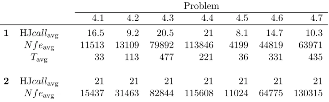
Table 1: Overall performance of 1 - ‘MS+m-HJ-f’ and 2 -Multistart Problem
4.1 4.2 4.3 4.4 4.5 4.6 4.7
1 HJcallavg 16.5 9.2 20.5 21 8.1 14.7 10.3
N f eavg 11513 13109 79892 113846 4199 44819 63971
Tavg 33 113 477 221 36 331 435
2 HJcallavg 21 21 21 21 21 21 21
76
M
.
F
er
n
an
d
a
P
.
C
os
ta
et
al
.
Table 2: Global and local optimal solutions of Problems 4.1 – 4.7, for 1 - ‘MS+m-HJ-f’ and 2 - Multistart Problem
4.1 4.2 4.3 4.4 4.5 4.6 4.7
1 global SR (%) 100 100 100 53.3 100 93.3 100
favg -6.66639367 189.29356 -13.401916 -0.94347611 2.0002495 7.66717368 4.57968167
HJ−N f eavg 590 1495 4929 4281 458 2205 6398
local SR (%) 80 6.7 73.3 90 6.7 100 20
favg -5.00000000 291.7582 -4.258899 -0.82372939 2.236262 8.24025030 5.80807333
HJ−N f eavg 519 2122 2986 5605 527 2813 3968
local SR (%) 70 46.7 13.3
favg -0.75059195 8.47635986 5.78054525
HJ−N f eavg 6323 1904 3712
local SR (%) 13.3
favg 7.82312050
HJ−N f eavg 5888
2 global SR (%) 100 100 100 53.3 100 93.3 100
favg -6.66645687 189.29288 -13.402434 -0.93642209 2.00011607 7.66689366 4.57966552
HJ−N f eavg 578 1443 4312 4971 413 2623 6401
local SR (%) 100 6.7 53.3 93.3 33.3 86.7 43.3
favg -5.00000000 285.0729 -4.258899 -0.82377402 2.23620740 8.23806018 5.80810378
HJ−N f eavg 637 2343 2783 6393 355 3635 3327
local SR (%) 66.7 46.7 36.7
favg -0.75279172 8.47622132 5.78100359
HJ−N f eavg 5250 2338 3922
Table 1 aims to compare the efficiency of both multistart kind algorithms. For each problem, the table shows averaged values over the 30 runs: HJcallavg (average number of local ‘mixed-HJ-filter’ calls), ‘N f eavg’ (average overall number of function evaluations of a run) and ‘Tavg’ (average overall time of a run, in seconds) only for our algorithm. For example, when solving Prob-lem 4.1, the ‘mixed-HJ-filter’ algorithm was invoked on average 16.5 times per run (out of a maximum of 21 (=Kmax+ 1)). The proposed ‘MS+m-HJ-f’ requires on average 11513 function evaluations and 33 seconds per run. On the other hand, we observe that the Multistart function invokes the local ‘mixed-HJ-filter’ procedure in every iteration and is consequently more expen-sive in terms of function evaluations than ‘MS+m-HJ-f’. We may conclude from the results of Table 1 that the proposed ‘MS+m-HJ-f’ behaves favorably when compared with the Multistart function.
Now, Table 2 reports for each identified optimal (global or local) solution: ‘SR’ (success rate - the percentage of runs that found that particular solution at least in one call to the local procedure, out of 30), ‘favg’ (the average of the best f values obtained during the runs where the solution was identified) and ‘HJ−N f eavg’ (the average number of function evaluations required by the ‘mixed-HJ-filter’ procedure while converging to those best solutions). Regard-ing the global solutions, the results show that both algorithms have equal ‘SR’ although the ‘favg’ produced by the Multistart function are slightly better than those obtained by our algorithm. We remark however that ‘MS+m-HJ-f’ is more effective since those values of ‘SR’ were obtained with less local ‘mixed-HJ-filter’ calls and fewer function evaluations (recall HJcallavg and ‘N f eavg’ respectively). As far as the local minima are concerned, we conclude that: i) both algorithms found almost the same number of minima (Multistart function did not find one of the locals in Problem 4.7); ii) ‘MS+m-HJ-f’ has a higher ‘SR’ in 3 out of 11 minima, whileMultistartfunction has a higher ‘SR’ in 5 (and equal ‘SR’ in 3 minima); iii)Multistart function produces slightly better average function values mostly (at a cost of more ‘mixed-HJ-filter’ calls and overall function evaluations, see Table 1).
5
Conclusions
method uses a specific pattern of points spread over the search space and in-tegrates a filter set methodology by solving a bound constrained bi-objective optimization problem each time it is invoked.
The new algorithm has been tested with benchmark problems and com-pared with theMultistartfunction from MATLAB, where we have integrated our ‘mixed-HJ-filter’ algorithm as the local solver in theMultistartfunction. From the comparison, we conclude that the herein presented multistart kind algorithm, based on the ‘mixed-HJ-filter’ algorithm, behaves rather well and is more effective, in the sense that it is able to identify the same number of solutions using on average less local ‘mixed-HJ-filter’ calls and fewer function evaluations than the other solver in comparison.
ACKNOWLEDGEMENTS.This work has been supported by FCT (Fun-da¸c˜ao para a Cˆencia e Tecnologia, Portugal) in the scope of the projects: PEst-OE/MAT/UI0013/2014 and PEst-OE/EEI/UI0319/2014.
References
[1] M.A. Abramson, C. Audet, J.W. Chrissis and J.G. Walston, Mesh adap-tive direct search algorithms for mixed variable optimization, Optimiza-tion Letters,3 (2009), 35–47.
[2] M.A. Abramson, C. Audet and J.E. Dennis, Jr., Filter pattern search algorithms for mixed variable constrained optimization problems. Pacific Journal of Optimization,3(3) (2007) 477-500.
[3] C. Audet and J.E. Dennis Jr., A pattern search filter method for nonlinear programming without derivatives, SIAM Journal on Optimization,14(4) (2004) 980–1010.
[4] F.P. Fernandes, M.F.P. Costa, E.M.G.P. Fernandes and A.M.A.C. Rocha, Multistart Hooke and Jeeves filter method for mixed variable optimiza-tion, International Conference of Numerical Analysis and Applied Math-ematics 2013, T.E. Simos, G. Psihoyios and Ch. Tsitouras (Eds.), AIP Conf. Proc. Vol. 1558 (2013) 614–617.
[5] R. Fletcher and S. Leyffer, Nonlinear programming without a penalty function, Mathematical Programming,91 (2001), 239–269.
[7] A. Hedar and A. Fahim, Filter-based genetic algorithm for mixed variable programming, Numerical Algebra, Control and Optimization,1(1) (2011), 99–116.
[8] R. Hooke and T.A. Jeeves, Direct search solution of numerical and statis-tical problems, Journal on Associated Computation, 8 (1961), 212–229. [9] T.G. Kolda, R.M. Lewis and V. Torczon, Optimization by direct search:
new perspectives on some classical and modern methods, SIAM Review,
45 (2003), 385–482.
[10] I.E. Lagaris and I.G. Tsoulos, Stopping rules for box-constrained stochas-tic global optimization, Applied Mathemastochas-tics and Computation, 197
(2008), 622–632.
[11] Y.C. Lin and K.S. Hwang, A mixed-coding scheme of evolutionary algo-rithms to solve mixed-integer nonlinear programming problems, Comput-ers and Mathematics with Applications,47 (2004), 1295–1307.
[12] G. Liuzzi, S. Lucidi and F. Rinaldi, Derivative-free methods for con-strained mixed-integer optimization, Report R. 11-11, Istituto di Analisi dei Sistemi ed Informatica “Antonio Ruberti”, CNR, Italy (2011).
[13] H.S. Ryoo and N.V. Sahinidis, Global optimization of nonconvex NLPs and MINLPs with applications in process design, Computers and Chem-ical Engineering,19(5) (1995), 551–566.
[14] M. Schl¨uter, J.A. Egea and J.R. Banga, Extended ant colony optimiza-tion for non-convex mixed integer nonlinear programming, Computers and Operations Research, 36 (2009), 2217–2229.
[15] V.K. Srivastava and A. Fahim, An optimization method for solving mixed discrete-continuous programming problems, Computers and Mathematics with Applications, 53 (2007), 1481–1491.
[16] I.G. Tsoulos and I.E. Lagaris, MinFinder: Locating all the local minima of a function, Computer Physics Communications, 174 (2006), 166–179. [17] I.G. Tsoulos and A. Stavrakoudis, On locating all roots of systems of
non-linear equations inside bounded domain using global optimization meth-ods, Nonlinear Analysis: Real World Applications,11(2010), 2465–2471. [18] C. Voglis and I.E. Lagaris, Towards “Ideal Multistart”. A stochastic ap-proach for locating the minima of a continuous function inside a bounded domain, Applied Mathematics and Computation,213(2009), 1404–1415.