DISSERTAÇÃO Neoclassical Transport of Particles in Magnetic Confined Plasmas

(1)

DISSERTAÇÃO

Neoclassical Transport of Particles in Magnetic Confined Plasmas

Felipe Nathan de Oliveira Lopes

Brasília, Março de 2017

(2)

(3)

(4)

FICHA CATALOGRÁFICA

LOPES, FELIPE NATHAN DE OLIVEIRA

Neoclassical Transport of Particles in Magnetic Confined Plasmas [Distrito Federal] 2017. xvi, 78 p., 210 x 297 mm (IFD/UnB, Mestre, Mestrado em Física, 2017).

Dissertação - Universidade de Brasília, Instituto de Física.

1. Plasmas 2. Confinamento Magnético

3. Transporte anômalo 4. Dissertações da PG-IFD

I.IFD/UnB II. Título (série)

REFERÊNCIA BIBLIOGRÁFICA

LOPES, F. (2017).Neoclassical Transport of Particles in Magnetic Confined Plasmas. Dissertação, Instituto de Física, Universidade de Brasília, Brasília, DF, 78 p.

CESSÃO DE DIREITOS

AUTOR: Felipe Nathan de Oliveira Lopes

TÍTULO: Neoclassical Transport of Particles in Magnetic Confined Plasmas. GRAU: Mestre em Física ANO: 2017

É concedida à Universidade de Brasília permissão para reproduzir cópias desta Dissertação e para empres-tar ou vender tais cópias somente para propósitos acadêmicos e científicos. Os autores reservam outros direitos de publicação e nenhuma parte dessa Dissertação pode ser reproduzida sem autorização por escrito dos autores.

Felipe Nathan de Oliveira Lopes Instituto de Física - IFD

Universidade de Brasília (UnB) Campus Darcy Ribeiro

(5)

Agradecimentos

Eu gostaria de dedicar este trabalho, primeiramente, ao meu professor e orientador, Ivan Ferreira, que mesmo nesta situação peculiar com a qual eu me encontro, conti-nuou com o trabalho apesar do esforço extra, e que no decorrer da minha graduação me ensinou coisas nao somente relacionadas ao conteúdo acadêmico mas também, e tão importante quanto, da vida.

Eu dedico também aos meus pais, Katia Aparecida e Gilson de Oliveira, e meu irmão, Yuri de Oliveira, que estiveram sempre do meu lado nos momentos em que nada fazia sentido para mim, e ainda continuam, porque as coisas ainda não fazem tanto sentido quanto eu acredito que deveriam fazer, por todo o carinho e atenção que eles me deram eu serei eternamente grato. Dedico à minha esposa, Estel Villaronga, que entrou na minha vida de uma maneira particular e tem sempre me apoiado, e que, por algum motivo, enxerga o sentido das coisas que eu nao sou capaz de enxergar. Dedico à todos os meus amigos, da minha cidade natal, Gama, onde eu cresci e aprendi o conceito de amizade, especialmente ao Caio e ao "bonde do Voyagem".

Dedico também aos meus amigos e companheiros da Universidade de Brasilia, aos que se foram, e aos que ainda estao por aqui, eles fazem definitivamente parte de uma importante e inesquecível etapa da minha vida. Lucas, Lilah, Rodrigo, Patricia, Artur, Suzane, Piri, e a muitos outros. Um agradecimento especial também à Coordenação de Aperfeicoamento de Pessoal de Nível Superior, CAPES, pelo apoio financeiro e pelo seu trabalho no fomento à pesquisa de pós-graduação stricto sensu no Brasil.

(6)

RESUMO

Plasmas confinados em diferentes topologias magnéticas são uma tarefa importante na busca pela Energia de Fusão. Hoje em dia, as formas mais estudadas de Fusão Termonuclear Controlada focam em Confinamento Inercial, Stellarators e Tokamaks. No presente trabalho, estudaremos os diferentes mecanismos de transporte presentes nos plasmas toroidalmente confinados. Vamos rever a teoria a partir dos conceitos básicos de transporte de plasma, até as peculiaridades presen-tes em plasmas toroidalmente confinados, conhecido como tokamak. Na fronteira do modelo de transporte mais realista, a questão do transporte anômalo será tratada com a teoria do transporte turbulento, no âmbito da teoria girocinética. O uso de ferramentas computacionais auxiliará na análise do impacto das microinstabilidades no fluxo de partículas e calor, e auxiliará na validação dessa abordagem, feita com uma análise da literatura.

ABSTRACT

(7)

LIST OF FIGURES

1.1 Biding energy for different isotopes [reference:Pearson Prentice Hall] ... 4

1.2 Lawson curve for the D-T reaction [reference:Stanford] ... 6

2.1 Z pinch. Yellow represents the current direction, and purple the magnetic field [credit: DaveBurke]. ... 8

2.2 ✓ pinch. Purple represents the current direction, and yellow the magnetic field [credit: DaveBurke]. ... 8

2.3 Torus. The blue arrow represents the toroidal direction and red the poloidal direc-tion. ... 9

2.4 Stellarator design [credit: IPP] ... 9

2.5 cross section view of the ITER [credit: iter.org]. ... 10

3.1 Diffusion level as function of collisionality regime [reference:Jan Mlynar] ... 33

4.1 Archetype of dissipation pathways within turbulent framework[P H Diamond1 et. al.] ... 38

4.2 ITG instability[credit:Aaron Scheinberg] ... 45

4.3 ETG saturation and streamers formation[credit:20th IAEA Fusion Energy Confe-rence] ... 46

4.4 Trapped particle mode instability[credit:Ben Dudson] ... 47

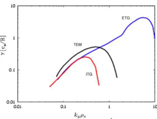
4.5 Range of instability growth rate, , for different microninstabilities range [cre-dit:F. Jenko] ... 48

5.1 Data parallelism scheme for SIMD architecture. [credit: Intel]... 50

5.2 Data parallelism scheme for MIMD architecture. [credit: Colin M.L. Burnett] ... 51

5.3 Distributed shared memory scheme. [credit: Blaise Barney] ... 52

5.4 OpenMP Fork-Joint mechanism. credit: Blaise Barney... 52

5.5 Scheme of a submission process. [credit: Brandon Barker] ... 53

5.6 Global GENE simulation of AUG reactor. credit: genecode.org ... 54

6.1 Formation of enhanced modes in a tokamak scenario [credit: CEA] ... 62

6.2 The f β _{behavior observed in a power spectra of GENE simulation [credit: M} Mavridis] ... 63

6.3 Heat flux fluctuations in normalized scales for aR/LT = 6.5[credit: M Mavridis] 64 6.4 Ion heat flux underprediction in GYRO simulation of DIII-D [credit: C. Holland ] . 65 6.5 Negative frequency versus toroidal mode number and radial position [credit: T. Görler ]... 66

(10)

(11)

(12)

LIST OF SYMBOLS

Latin Symbols

Q Heat Flux

Vζ Toroidal Flow Velocity

~ Planck’s Constant

Greek Symbols

Γ Particle Flux

i Heat Diffusivity Electrical conductivity Ψ Flux Surface

⌫ collisional frequency

µ Magnetic Momentum Π Viscous Stress

Instability Growth Rate

! Instability Frequency

Dimensionless Constants

e Euler Constant

⇡ pi Constant

i Imaginary Number

Acronym

ITER International Tokamak Experimental Reactor JET Joint European Torus

(13)

1 INTRODUCTION

1.1 INTRODUCTION

The increasing global energetic consume is reaching limits intolerable for the old means of power production to provide sustainable electric energy. One of the most promising candidate to deal with this issue is the Thermonuclear Controlled Fusion. The aim of this dissertation is to provide an insightful understanding of the transport phenomena in Thermonuclear Plasmas, most precisely anomalous and turbulent transport.

Transport is the study of the mechanism in which mass, energy and momentum are exchan-ged in a given system. In complex systems such as magnetically confined plasmas, non intuitive effects may appear due to the complexity of the interaction of the different particles with the back-ground field and from the field with the particles. Disregarding the already known non orthodox effects of transport phenomena in magnetized plasmas, new mechanisms that does not fit in the old measurements are treated. Anomalous transport can be considered as the set of divergence of orders of magnitude between neoclassical prediction and real measurements. It is mostly caused by turbulence motion steered by micro-instabilities.

The structure of this monograph is as follows. Chapter 1 discusses a brief introduction to the topic. Chapter 2 presents the mechanism of plasma confinement from the most basic approach, up to the classical model. Chapter 3 discuss more realistic approach to the transport description, and chapter 4 introduces the gyrokinetic solution to the anomalous issue. Chapter 5 introduces and explains the numerical approach, and chapter 6 deals with examples, concluding with chapter 7.

1.2 THE QUEST FOR ENERGY

(14)

impact on global warming, the rate of increase in consumption and population growth represent a real treat to a sustainable evolution.

To discontinue technological progress is unfeasible and unreasonable. A new strategy in the approach to progress needs to be taken. A brighter future is foreseen only if together with an improvement of the status quo of the environmental panorama. Innovative energy sources are needed and more efficient energy storage mechanism needs to be developed, in order to minimize the effects caused by the enormous amount of gases released in the atmosphere during the last century and to mitigate any other effect that may have impact in the environment whatsoever.

1.3 NUCLEAR ENERGY

In 1932, Ernest Rutherford was reported to have discovered that lithium atoms, when split by protons, could release energy, in agreement with the mass-energy equivalence principle esta-blished by Albert Einstein (Richard Rhodes, 1986). The late discovery of the neutron by James Chadwick opened a path to what is known as the atomic era, where the nuclear energy was used as an alternative form of electric energy and as a novel weaponry mechanism.

Nuclear energy is considered as all the energy that is provided by the break down or fusion of nuclear particles (John R. Lamarsh, 2001). Two approaches are known, the one involving the breakdown of heavy atom, known as Nuclear Fission and another one associated with the fusion of light nuclei, known as Nuclear Fusion.

1.3.1 Nuclear Fission

Nuclear Fission is a subatomic process in which a heavy nucleus undergo a decay to another nuclei with lighter atomic mass and is followed by the release of an amount of energy correspon-dent to the difference in the biding energies of the primary nucleus and the two remaining nuclei. It is important to understand that a Nuclear Reaction is caused by neutron bombing the heavy and unstable nucleus, also know as radioactive decay, described as a spontaneous break of the nucleus due to quantum mechanics effects acting within the subatomic particles. An example of Nuclear Reaction, followed by the nucleus split and energy release is described as follows

1

0n+23592 U!14192 Ba+9236Kr+ 310n+Energy (1.1)

A neutron collides with the nucleus of235

92 U and as a result the nucleus is split in two lighter

(15)

The issue with the Nuclear Fission processes is the reaction chain. The three neutrons released in the reaction 1.1 collide with three new nuclei and give rise to a chain of reaction that increases its energy release exponentially. Controlled Nuclear Fission is a deep and complex field of study that requires deep knowledge of the interplay of nuclear forces and feedback mechanism to the proper management of the chain reaction. Another important issue with Nuclear Fission is the radioactive waste. Since the products of the Nuclear Reactions are in its majority radioactive, the process generates enormous amounts of material radioactively contaminated, and in cases of human negligence or unpreparedness, leaks of contaminated material to the environment are cause of concern and fear.

1.3.2 Nuclear Fusion

Contrary to the Nuclear Fission, Nuclear Fusion is a process in which two light nuclei, in general Hydrogen isotopes, are put together and combine, originating a heavier element, generally helium. Nuclear Fusion is the main form of energy release in all the stars in the Universe and the pursuit of this form of energy on earth has been driving a considerable effort from humankind. In order to maximize the effective cross section, the most effective elements used are the Deuterium,

2

1H, and the Tritium,31H. The reaction is described as follows

2

1H+31H!24 He+10n+Energy (1.2)

In the case of heavenly bodies like stars, it is important to notice that the main chain of fusion reaction of such bodies with the mass of the sun or less, is the proton-proton chain reaction.

1

1H+11H!22 He+ !12 H+e++⌫e+ 0.42M eV (1.3)

It is necessary to remember also that, due to the high value of mass, the gravitational pressure of the sun exert enough force to keep the plasma confined, and high values of kinetic energy are possible to be achieved by the protons due to the counterbalancing of the gravitational effect. In the case of earthly magnetic confinement, the most common approach is using magnetic fields, and as an alternative, a reaction with Deuterium Tritium is chosen due to its high cross section and higher values of energy released.

Figure 1.1 shows us the different nature of the biding energy for different atomic numbers. It is seen that the energy released per nucleon in the case of fusion reactions is larger than the energy released in the fission case.

(16)

Figura 1.1: Biding energy for different isotopes [reference:Pearson Prentice Hall]

of the two charged particles (Shultis, J.K. 2002), this is possible due to a mechanism known as the Quantum Tunneling.

In Quantum Mechanics, particles are described as wave functions and their temporal behavior is implied from the Schrödinger wave equation. In this scenario, the particle’s observables is extracted as the result of a probability density function.

i~@Ψ(r, t)

@t =

_~2

2µ 5

2 ₊_V₍_{r, t}₎

Ψ(r, t) (1.4)

Schrödinger equation (1.4) describes the time evolution of the quantum state of a system, where Ψ(r, t) is the wave function, and V(r, t) represents the potential in which the particle is submitted. By means of Fourier analysis, Equation 1.4 can be solved and the resulting equa-tion 1.5 is the wave-like direct soluequa-tion of Schrödinger equaequa-tion, validating a non corpuscular interpretation.

Ψ(r, t) = 1 (p2⇡)3

Z

Φ(k)ei(k·r wt)d3k (1.5)

As a consequence of the mathematical formulation, particles are expected to interact in a pro-babilistic way with potential wells, and due to this mechanism, there is a non zero probability that when faced with a higher potential compared to its own energy, a particle may overcome it. This effect is known as Quantum Tunneling.

(17)

From the reaction 1.2, 17.58M eV is released as energy. The essential point of the Nuclear Fusion is that Deuterium is found in sea water, in the form of heavy water, and the Tritium can be easily bred, making therefore the reaction cheaper and more abundant. In order to fuse, the nuclei must be put close enough to overcome the electrostatic Columb potential. This means a certain amount of energy must be deposited on the system in order to achieve what is known as ignition. Ignition the point where the heat from the fusion reactions is enough to maintain the re-action ongoing without external input and considering all the possible losses. The field of Physics concerned with the study of such reactions is called Plasma Physics.

Plasma Physics is the field of physics concerned with the study of matter when electrons are detached from atoms and behave freely from it.

Due ti the high temperatures required and the complex non linear dynamics of the Plasma, this alternative as an energy source is seen almost as an utopia, but if there is something that humankind learn through the centuries is that a dream dreamt together becomes reality. Due to the absence of uncontrolled chain of reactions and almost no radioactive waste, Nuclear Fusion has an enormous advantage when compared to Nuclear Fission.

1.4 THERMONUCLEAR CONTROLLED FUSION

Thermonuclear Fusion is considered the way to achieve nuclear fusion by means of extremely high temperatures, in order to fulfill the Lawson Criteria. The Lawson Criteria measures a relation between the plasma electron densityneand the energy confinement time ⌧E and gives condition for a fusion reaction to reach ignition. More precisely, the Lawson criteria is a not-so-rigorous principle, as described by J. D. Lawson himself, utilized to envisage the range of values of density and energy confinement time of a burning plasma in order to achieve a self sustained reaction. The equation represents a power balance in thermonuclear reactors in order to get an approxima-tion of the referred quantity.

In the case of the Deuterium-Tritium reaction, for temperatures of the order ofT = 14keV, the Triplet Product (J. D. Lawson, 1957) can be approximated by the following relation

nT⌧E 3·1021KeV s/m3 (1.6)

(18)

Figura 1.2: Lawson curve for the D-T reaction [reference:Stanford]

Contemplating the above restrictions, some concern must be addressed to the approach in which way the Plasma will be confined, and for how long its facing components will cope with hundreds of million degrees and, furthermore, the best way the avoid instabilities.

(19)

2 PLASMA CONFINEMENT

The study of toroidally confined Plasmas cannot be accurately performed without a deep un-derstanding of Magnetized Plasma. The need for it comes from the fact that, typical plasma temperature in a fusion device are of the order of,10KeV, as expected in ITER. In such scenario, no known material is capable of coping with such temperatures and therefore, a broad expertise in magnetically confined plasmas is required in order to avoid the melting of plasma facing com-ponents.

Whilst dealing with magnetized plasma, a focus in fully ionized matter is required in order to maintain the relevance in regard to core fusion devices. The plasma consist of unbounded ions and electrons, forming a quasi-neutral fluid, which means that in a macroscopic first order approximation, the plasma can be considered neutral. When closely analyzed, a parameter known as Debye length plays an important role in defining first and further orders of approximation for of plasma neutrality analysis. The Debye length is a measure of the persistence of electrostatic effects in the plasma, in practical terms, it gives us the scale in which the quasi-neutrality can be considered valid. The fact that the plasma does not allow macroscopic charge separation does not mean that there are no electrostatic fields present, in most of the cases a property known as self-organization, vastly present in magnetized fusion plasma, allows the appearance of structures carrying significantly high values of electric fields (M. Mavridis, 2014).

2.1 CONFINEMENT MODELS

Within the MCF approach, different devices designs are often used. Magnetic mirrors pursue the confinement by means of the mirror effect of magnetic fields and the formation of magnetic bottles, structures formed when two diverging magnetic fields are put together. The pinch effect is described as a compression of a filament of current by means of magnetic forces. In this con-cept, two main devices are studied, the ✓andZ pinch machines. In theZ pinch machine, figure 2.1, the current, (yellow), flows in the axis direction, and the magnetic field points to the poloidal direction. Meanwhile in the✓ pinch, figure 2.2, the magnetic field, (purple arrow), is the one to

stream in the axial direction, whereas the current points to the poloidal direction.

(20)

Figura 2.1:Zpinch. Yellow represents the current direction, and purple the magnetic field [credit: DaveBurke].

Figura 2.2:θpinch. Purple represents the current direction, and yellow the magnetic field [credit: DaveBurke].

In topology theory, a Torus, figure 2.3, is a three dimensional solid obtained by the revolving of a circle around a co-planar axis. When used to mold the shape of the plasma where the nuclear fusion reactions are taking place, the torus shape presents the advantage of allowing the magne-tic field to have, also, a toroidal geometry. Following the Poincaré–Hopf theorem of differential topology and the Hairy Ball theorem of algebraic topology and its implications in topological pro-perties of n-dimensional folds, the torus is a solid which possesses an Euler characteristic number equal to zero ( Jean-Paul Brasselet, 2009), which means we can drawn a continuous vector field in its surface with non vanishing points. It is important to fulfill this criteria because the magnetic field formed in this shape cannot have any vanishing point, since it would lead the plasma to be dislodged from its stability.

(21)

Figura 2.3: Torus. The blue arrow represents the toroidal direction and red the poloidal direction.

drives in order to avoid the losses to the containment. The losses are avoided by the fact that the planar cross sections are twisted in order to form a Möbius strip. This way, particles experiencing an upward drift in one side will be counterbalanced by a downward drift in the other side, creating an almost zero balance in the total drift.

Figura 2.4: Stellarator design [credit: IPP]

Another solution to the drift problem is to bend the axial magnetic field lines in a poloidal direction, red line in figure 2.3, in this way, the field lines will created a flux surface rounding the whole torus, and a counteraction will be generated in order to avoid the drift losses. This approach is applied in the Tokamak reactors.

2.1.1 ITER and the tokamak model

Tokamak is the Russian acronym of theipsis litteris"to_roidalch_{amber with}ma_gneticc_oils".

(22)

Following laser scattering measurements, and with the confirmation of the higher temperatu-res and stability of the tokamak model, the Joint European Torus (JET) began to be constructed in 1973. There are few operational tokamaks around the globe, one of them, the TCABR, can be found in the University of Sao Paulo, USP. The tokamak fast became the most used confi-nement approach around the world. The ITER, figure 2.5, latin for "the way", and acronym of

I_nternationalT_hermonuclearE_xperimentalR_eactor, started to be assembled in 2015, is the world

largest MCF device. Expected to deliver fusion electricity by the end of 2030 (European Fusion Development Agreement, 2006).

Figura 2.5: cross section view of the ITER [credit: iter.org].

The use of a current driven in the tokamak leads the plasma to a series of instabilities. Most of this instabilities are due to Magnetohydrodynamic (MHD) modes,i. e. this modes degraded the confinement and can lead to plasma disruption. Microturbulences driven by ions also contributes to plasma disruption scenario.

The full scenario of instabilities and degradation in ITER may be stabilized by a set of complex feedback controls that increase the complexity of the machine.

2.2 DYNAMICS IN MAGNETIZED PLASMA

(23)

Let us consider the Lorentz equation for a particle with chargequnder the action of a force_F~

due to the electric and magnetic fields_E~ _and_B~

dp

dt =F =q(E+v⇥B) (2.1)

where ~pis the momentum of the particle and ~v its velocity. It is easy to see that under the influence of a electrostatic field, eq.2.1 results

r(t) = 1 2(

qE m )t

2₊_v

0t+r0 (2.2)

wherer0is the initial position andv0is the initial velocity. In this case the particle has a

cons-tant acceleration, qE

m. For a magnetostatic field the trajectory is found by separating the velocity of the particle in parallel and the perpendicular direction of the magnetic field. The movement in the direction of the magnetic field is not affected, and we are left with the perpendicular component of the resulting Lorentz equation

dv? dt =

q

m(v?⇥B) (2.3)

considering _Ωc = q_mB, and considering that Ωc is constant in a constant magnetic field, known as cyclotron frequency, we can observe that 2.3 can be integrated to

v? =Ωc⇥rc (2.4)

where~rc is the the particle position related to the center of the gyration point, in a plane per-pendicular to _B~_{. Equation 2.4 represents the rotation of the position} _~_rc_{. The resulting motion}

of the particle is given by the superposition of the uniform motion along _B~ _{and and the circular}

motion perpendicular to _B~_{. The radius in which the particle gyro-rotates is known as Larmor}

radius, defined as⇢= mv?

qB .

The analysis of_E~ _{together with}_B~ _{is done by separating the components of}_~_v _and_E~ _parallel

and perpendicular to_B~_{. In the same direction of the magnetic field, we have}

rk(t) = 1 2(

qEk m )t

2₊_vk₍₀₎_t₊_rk₍₀₎ _(2.5)

(24)

E? = E?⇥B

B2 ⇥B (2.6)

one can finally arrive in the description of the particle motion unconstrained to a coordinate frame

v(t) = Ωc⇥rc+

E?_⇥B B2 +

qEk

m t+vk(0) (2.7)

In equation 2.7, the term E?⇥B

B2 represents theE⇥B drift. The result motion of the particle is a cycloid.

It can be observed that, when E and B are perpendicular a confined plasma, a drift found in the second term on RHS of equation 2.7, is created. Thus a possible loss of material in thev(t) direction is foreseen and the confinement may be terminated.

2.3 TOROIDAL CONFINEMENT

Toroidal confinement is of great importance because it was the chosen configuration in which most of the efforts to develop sustained nuclear power are put nowadays. Two important topics in toroidal confinement must be contemplated for the scope of this work, firstly, classical motion of particles in non uniform magnetic fields, and secondly, the equilibrium of forces in a toroidaly magnetized plasma.

2.3.1 Classical Analysis

An important consideration that must be done is the drift in slowly changing fields. In the case of a toroidally confined plasma, the geometry of the magnetic field does not allow it to have a continuous value in all the space. A drift is generated due to changes in the magnetic field intensity along the particle orbit.

First we need to consider the magnetic field, our object of study in this section, varying with the position vector in reference to the gyrocenter direction,rL(t). The motion of the particle is in the direction of the magnetic field, and the position and velocity vector can be decomposed in the gyrocenter direction, related to the field line, and around the field line.

B(x(t)) =B(x(t)) +rL(t)) =B(x(t)) + (rL(t))·r)B (2.8)

(25)

md[vgc(t) +vl(t)]

dt =q[E(xgc(t)) + (rl(t)·r)E] +q[vgc(t) +vl(t)]⇥[B(xgc(t) + (rl(t)·r)B] (2.9)

And the first cyclotron motion can be extracted as

mdvl(t)

dt =qvl⇥B(xgc(t)) (2.10) and

mdvgc(t)

dt =q[E(xgc(t))+(rl(t)·r)E]+q[vgc(t)⇥[B(xgc(t) + (rl(t)·r)B] +vl(t)⇥(rl(t)·r)B] (2.11)

Now, decomposing the gyrocentric velocity in two perpendicular components

vgc(t) =

(

v?gc(t) vkgc(t)B

)

(2.12)

The time derivative of the left hand side of 2.12 is taken as the sum of the two components in the right hand side. Form here, a relation to the derivative of the magnetic field direction can be taken

dB dt =

@B

@s ds

dt =vkgc(t)B ·rB (2.13) Wheresrepresents a field element line. We can, now, decompose Lorentz equation along and perpendicular toB

mdvkgc(t) dt =q

h

Ek(xgc(t)) +_hvl(t)_⇥(rl(t)·_r)B_i_ki (2.14)

and for the perpendicular direction

m[dv?gc(t) dt +v

2

kgc(t)B·rB] =q

2

6 4

E?(xgc(t)) +vgc(t)_⇥B(xgc(t)) +_hvl(t)_⇥(rl(t)·_r)B_i_?

3

7

5 (2.15)

In a more generic form

mdv?gc(t)

dt =F?+qvgc⇥B (2.16)

~

(26)

F? =q[E?(xgc(t)) +_hvl(t)_⇥(rl(t)·_r)B_i_?] mv2_kgc(t)B·_rB (2.17)

If we consider thatv?gc(t)has a slow time dependence, we can approximate the perpendicular gyrocentric velocity

v?gc(t)_'vF _⌘ F?⇥B

qB2 (2.18)

Considering now an approximation to the first guess,v?gc(t) =vF+vP and developing based on the above assumption

mdvF +vP

dt =F?+q(vF +vP)⇥B (2.19)

and considering also that dvP

dt ⌧

dvF

dt we arrive in the general polarization drift

vP = m qB2

dvF

dt ⇥B (2.20)

In the case that we have~vF =E~ ⇥B~ the polarization drift becomes

vP = m qB2

dE

dt (2.21)

If, now, we consider the drift generated by the curvature of the magnetic field, one should just express how the perpendicular force is described in 2.18. Making a gyro average of the perpendicular force in cylindrical coordinates, we get

hF?_i= 2|m|( 1 2⇡

I

@B

@rrd✓) = |m|(rB)? (2.22)

The grad B drift becomes, so

vrB = |m| q

(_rB)_⇥B

B2 (2.23)

Equation 2.23 has a dependence in the particle charge, which means that electrons and ions drift in opposite direction and generate a net electric current.

A centrifugal force associated with the movement of the particles is generate due to the shape of the field. The force has the following form

Fc =

mv2

kgc

(27)

Equation 2.24 represents the force associated with the curvature of fields line, and when subs-tituted in 2.18 we get

vc = 1 qB2

mv2

kgcR

R ⇥B (2.25)

Where R is the radius of the curvature. In a tokamak, it will be associated with the major radius.

It is important to understand that, the transport study is directly connected with the type of confinement constraining the particles. As seen above, classical electrodynamics provides us with a rustic approximation to the study of particles behavior in confined plasmas, but the fluid like nature of the plasma makes the study of transport relatively more complicated. A deeper study of transport will be done in the next chapter. In the present one, we will restrict ourselves with a phenomenological first order approximation description of the particle dynamic.

2.3.2 Magnetic Equilibrium and the Grad Shafranov Equation

In order to achieve a sustained fusion reaction, an equilibrium between the plasma pressure and the toroidal magnetic field must be achieved. Notwithstanding the instabilities generated by the toroidal geometry, that further on will be discussed, an internal balance between the plasma pressure and the forces from the magnetic field must be met. Such behavior is described by the Grad Shafranov equation.

Consider the plasma pressure to be isotropic, which means that the pressure tensor can be reduce to a diagonal matrix, the plasma momentum equation can be reduced to

J_⇥B =_rP (2.26)

WhereJ is the current density,B is the Magnetic field andP is the pressure. By considering J, B, andP represented by a single-valued function of Ψ, the poloidal magnetic flux function determined by each poloidal flux associated with individual flux surfaces, one may represent the force balance equation in terms of the new variableΨ.

Before proceeding, some assumptions are made. P is constant along a magnetic field line. This assumption is important because, sinceP is represented as a function ofΨ, the latter must, also, be constant along a magnetic field line, and therefore, P can be expressed individually by Ψ.

B·_rP = dP

(28)

In the toroidal direction, the space derivative of P vanishes, and from the plasma current description, considering R the radial direction, Z the toroidal direction, andf =RBφ(R, Z), we can write theRandZ components of the current in terms off as

JR = 1 R

@f

@Z (2.28)

and

JZ = 1 R

@f

@R (2.29)

and, considering 2.28 and 2.29 inJZBR JRBZ = 0, we have

@f

@RBR+

@f

@ZBZ = 0 (2.30)

Which means,B·_rf = 0, in other words,f can, also, be described as a function ofΨ.

Considering the balance in the R direction, using the proper terms to express the current density and magnetic field, and considering thatP andf are functions ofΨ, one may arrive in

∆⇤Ψ= R2dP dΨ f

df

dΨ (2.31)

described in another manner,

@2Ψ

@Z2 +R @ @R(

1 R

@Ψ

@R) = R

2dP

dΨ f df

dΨ (2.32)

Equation 2.32 is known as Grad Shafranov equation, and it is used in order to describe equili-brium conditions for axisymmetric toroidal magnetized plasmas. This equation is widely used in plasma simulation codes in order to minimize the value of the total energy of the plasma pressure and magnetic field system, and find a suitable magnetic geometry that satisfies stability.

2.4 KINETIC THEORY

(29)

The kinetic theory brings the microscopic effects of particles into the macroscopic world th-rough the use of statistical tools. The averaging out of microscopic effects lead to statistic kinetic effects, and these may lead us further to a particle-fluid characterization of the plasma.

In this section, one may see how statistic tools help us to extract information from the micros-copic system and which is the role of Boltzmann and Vlasovequation in the description of the plasma.

2.4.1 Distribution Function and Boltzmann Equation

Consider a 6 dimensional phase space containing the 3 coordinates of space,r, and 3 coordi-nates of velocities,v, of a finite number of particles in a volumed3_rd3_v_{. Describing the number of}

particle in such a infinitesimal section by d6_N₍_{r, v, t}_{), the function that represents the statistical}

distribution is denoted by the the number of particles over the volume of the phase space.

It is worth to notice that macroscopic quantities such as number density and average velocity may be averaged out from the distribution function as follows

n(r, t) =

Z

f(r, v, t)d3v (2.33)

Wheref(r, v, t)is the distribution function of the particles and the integral symbol stands for a triple integral. The average velocity comes out as

u(r, t) = 1 n(r, t)

Z

vf(r, v, t)d3v (2.34)

Under specific considerations, the distribution function describes the change in the observable parameter. The qualitative construction of such relation is describe as following.

Consider the accelerationa = F/mgenerated by a force F, acting in the volume element in the phase space of the system. Such force will make the element move in the phase space. The geometry of the volume element will change after a timetto a statef0 as

[f(r0, v0, t+dt) f(r, v, t)]d3rd3v = 0 (2.35)

(30)

f(r+vdt, v+adt, t+dt) =f(r, v, t) +



@f(r, v, t)

@t +v·rf(r, v, t) +a·rvf(r, v, t) dt (2.36)

Equation 2.36 can be rewritten as

@f(r, v, t)

@t +v·rf(r, v, t) +a·rvf(r, v, t) = 0 (2.37) Known as the Boltzmann equation in the absence of collisions.

For a better description of transport phenomena, interactions must be taken into account, the change in the phase space configuration due to collision modifies the aspect of the finite element, introducing or withdrawing particles from its interior. Since the total balance of particles is in principle unknown, a collisional operator, representing the rate of change of the main distribution function, is introduced in the equation.



f(r, v, t) t _colld

3_rd3_vdt _(2.38)

The modified equation thus becomes

@f(r, v, t)

@t +v·rf(r, v, t) +a·rvf(r, v, t) =

✓

f(r, v, t) t

◆

coll

(2.39)

It is important to remember that the collisional model above described is a roughly, but accu-rate, approach and that more rigorous description exists,e.g. the Fokker-Planck model.

2.4.2 Vlasov Equation

By taking into account electric and magnetic fields, a more precise approximation can be for-mulated.

The Vlasov equation is described as the partial differential collisionless Boltzmann equation in the presence of macroscopic electric and magnetic fields.

@f

@t +v·rf + 1

(31)

2.5 A FIRST APPROACH TO TRANSPORT THEORY

The transport theory is responsible for the study of transfer of quantities between and within a set of systems or a given system. Mass, momentum, and energy are quantities frequently analyzed as macroscopic variables of interest in order to describe plasma dynamics.

From the previously described Boltzmann equation and the particle distribution function, one may, by means of solving the latter with the help of the former, arrive in a set of equations sui-table to guide us in understanding how the transport phenomena occurs in magnetized plasma. The plasmamacroscopic transport equationsare extracted directly from the Boltzmann equation in form of moments of the distribution function. As a result we have a set of equations known as moments of the Boltzmann equations. This moments can be associated with conservation equati-ons of mass, momentum and energy, the objects of study of this section.

2.5.1 Qualitative analysis of moments of Boltzmann equation

The moments of the Boltzmann equation arise as an attempt to extract macroscopic properties of the system by means of the distribution function and the Boltzmann equation. A way to do so is to take the average of the distribution function in the Boltzmann equation considering the phase space of the independent parameter of the physical variable in consideration. Suppose that a given physical quantity, ⇣(v), is proposed to be studied by the method of moments. First, one should average it out by multiplying it by the Boltzmann equation and integrating it in all space of velocities, then dividing the result by the particle number density.

Consider the Boltzmann equation 2.39, multiplying it by⇣(v)and integrating over the space of velocities we get

Z

v

⇣@f @td

3_v₊

Z

v

⇣v·_rf d3v+

Z

v

⇣a·_rvf d3v =

Z v ⇣ ✓ f t ◆ coll

d3v (2.41)

We now Independently analyze each of the terms. The first term can be rewritten as

Z

v

⇣@f @td

3_v ₌ @ @t(

Z

v

⇣f d3v)

Z

v f@⇣

@td

3_v _(2.42)

Considering that⇣(v)does not depend on time, the last term vanishes and using the standard notation of averages,_h⇣(v)_i, and making use of 2.33:

Z

v

⇣@f @td

3_v ₌ @

(32)

For the second term, the part containing the divergence vanishes due to the configuration of the velocity in the space phase, and likewise_r⇣(v)vanishes, since it is independent of the space variable. The second term then becomes

Z

v

⇣v·_rf d3v =_r·(n_h⇣(v)_i) (2.44)

The third term requires more attention. Assuming that the field of forces has divergence zero, i.e., the force component in a given direction is independent of the velocity in that same direction, and considering the expansion of the third term

Z

v

⇣ a·_rvf d3v =

Z

vr

v ·(a⇣ f)d3v

Z

v

f a·_rv ⇣d3v

Z

v

f ⇣_rv ·a d3v (2.45)

From equation 2.45, the first term of the right-hand side is a sum of three triple integrals , and each of this triple integrals result in zero, and the first integral in the right-hand side becomes

Z

v

⇣a·_rvf d3v = nha·rv⇣i (2.46)

Bringing together the separate result of the three terms, one is able to retrieve the general transport equation,

@

@t(nh⇣(v)i) +r·(nh⇣(v)i) nha·rv⇣i=

✓

t(nh⇣(v)i)

◆

coll

(2.47)

The right-hand side represents the rate in which collision modifies the quantity⇣and alter the

exchange of value .

2.5.2 Mass conservation

From this general principle, one may derive important relations that are helpful to understand how transport takes place within the constrains previous established. By firstly considering ⇣ = m, wheremis the mass of a given species, we have

h⇣_i=m (2.48)

(33)

rv⇣ =rvm = 0 (2.50)

Replacing these quantities in the general transport equation we have

@⇢m

@t +r·(⇢mu) = S (2.51)

Equation??is known as thecontinuity equation. The term⇢represents the mass densityn·m,

uis the linear velocity, andSrepresents the collision term.

By considering a collisionless scenario, dividing 2.51 by the mass m, and multiplying the whole equation by the charge of the specie, one may arrive at the conservation of the electric chargeequation

@⇢m

@t +r·J= 0 (2.52)

Where⇢=n·qis the charge density andJ=⇢uis the current density.

2.5.3 Momentum conservation

The conservation of momentum is extracted in a similar way as the mass conservation. Here, a more throughout analysis must be done in order to consider the standard variable⇣ =mv, being v =w+u, wherewis the random movement around the mean velocity, and_hw_i= 0.

Considering the acceleration in terms of the force and the mass, each of the terms can be reduced to

@

@t(nh⇣(v)i) =

@

@t(m n u) (2.53)

rv(m nhwiwji) = r· !Ψ (2.54)

n_hF_i= n(r, t)q(E + v_⇥B) (2.55)

(34)

n m Du

Dt =n q(E+u⇥B) r·

!

Ψ (2.56)

This is themomentum conservation equation. It roughly represents how the rate in change of momentum varies with the collision term .

2.5.4 Energy conservation

In a similar way as already considered, the energy transport equation can be extracted from the Boltzmann equation in a partial differential form. Here, the general quantity ⇣is replaced by

the particle kinetic energy mv2

2 . In this case we have to consider the velocity as a two component

quantity, and treat each term separately

@

@t(nh⇣(v)i) =

@ @t(

N !Ψ

2 +

m n u2

2 ) (2.57)

r·(n_h⇣(v)_i) =_r·(Q(2 +N

2 )

!

Ψu+ mnu

2

2 u) (2.58)

n_ha·_rv⇣i= q n u ·E (2.59)

And the collision term is

= ✓ @W @t ◆ coll (2.60)

representing the rate in which the energy is transferred among particles by collision effects.

Here, N represents the dimensional number in which the dyadic of pressure is considered, for isotropic cases it is considered unit. The quantityQis the heat flux, expressed as

Q=

Z

v mw2

2 w f d

3_v _(2.61)

Bringing up all the terms together and performing the necessary adjustments, we have

N 2

D!Ψ Dt +

2 +N 2

!

Ψr·u= _r·Q+ ·u (@W

@t )coll (2.62)

(35)

2.6 CONSIDERATIONS

From the equations above described, it is advantageous to compute two quantities, relating the moments extracted from the Boltzmann equation and the magnetic flux function, expressed in two important transport quantities in terms of the flux functionΨ.

hΓ·_rΨi=

⌧Z

v

d3vf u·_rΨ (2.63)

hQ·_rΨi=

⌧Z

v

d3_vm u2

2 f u·rΨ (2.64)

Equation 2.63 represents the flux surface average of the radial particle flux, 2.64 is the energy flux, and_h·_idenotes flux surface average.

(36)

3 TOKAMAK

3.1 REALISTIC TRANSPORT MODELS

It is important to observe that, although elegantly derived from fluid dynamics and electro-magnetic theory, the classical models of transport are not enough to describe the dynamics of the particles in a tokamak. The consideration of the toroidal magnetic geometry of the device plays an important role in most recent models, where effects due to the gradients of the field start to show the importance and impact of morphological considerations.

3.1.1 Classical Transport Operators

The former Vlasov equation needs to be modified in the sense that it must now account for effects like collisions. Classical and collision induced plasma current must be defined and irre-ducible levels of transport caused by Coulomb collision must be included. Two operators are considered. The Fokker-Planck coulomb collision operator makes the assumption that particles can only collide with each other and with other particles, bringing us to a rate change in the distribution function due to internal collisions, expressed as

C(f)_⌘

✓ @f @t ◆ ∆v = lim

∆t!0

f(x, v, t) f(x, v, t ∆t)

∆t (3.1)

The integro-differential form of the operator can be described as as

C(f)⇠= @

@v ·

h∆v_i ∆t f+

1 2

@2 @v@v

∆v∆v

∆t f+... (3.2)

The Operator is a scalar, invariant under rotation, and symmetric with respect to Galilean transformations, making it a rotationally symmetric, or isotropic, operator. When expressed in terms of the Rosenbluth Potentials, from the Rosenbluth-MacDonald-Judd form, and considering the specific changes in velocity vector due to coulomb collisions of particle "a"with background particle "b", one may get the form

C(f) = @f

@v ·Γab

h@Hb_i

@v f + 1 2

@2 @v@vΓab

@Gb

@v@vf (3.3)

WhereHbandGbrepresent the Rosenbluth potentials

Hb(v) = (1 +ma mb)

Z

d3v0 fb(v 0₎

(37)

Gb(v) =

Z

d3v0fb(v0)|v v0| (3.5)

And the factor_Γis represented as

Γ= q

2

aqb2ln(Λab) 4⇡✏0m2

a

(3.6)

Whereln(Λab)is the Coulomb logarithm. Another important consideration that must be done in regard to the collision of particles with a stationary background, is the Lorentz Collision Ope-rator expressed as:

CL(f) = ⌫(v) 2



@

@⇣(1 ⇣ 2₎@f

@⇣ +

1 1 ⇣2

@2f

@'2 (3.7)

Where⇣ = vk

v and' =tan

1vy

vx. For

h∆vi

∆t =⌫(v)v. This operator might be seen as a form of angular scattering in the velocity space.

From now on, one must be capable of recognizing important factors and a more precise des-cription of a tokamak plasma transport.

3.1.2 Electrical Conductivity within Lorentz operator

An important property that must be studied in order to precisely describe plasma inner me-chanisms is known as electrical conductivity. The electrical conductivity help us to quantify a material’s ability to allow transport of electric charges, be it electrons or ions. Following the Spitzer-Härm argument, the study of plasma conductivity is done by assuming the application of a Electrical field E in an infinite homogeneous plasma and analyzing its steady state current. Something with the formJ= Eis expected, being the conductivity. Making use of the Vlasov equation for the Maxwellian distribution function, one may get

q mE·

@f

@v =C(f) (3.8)

From a phenomenological point of view, a correct scaling with plasma parameters is found when we consider the electron momentum balance and a shifted maxwellian distribution. Inte-grating 3.8 inR

mvd3_v_{, resulting in} _nqE _mn_⌫_v_{, we get}

J = nqv = nq

2

m⌫E = E ⌘

E

(38)

the first order approximation of the plasma electrical conductivity is

0 =

nq2

m⌫ (3.10)

Any improvement in this conductivity will only add numerical coefficients to the very same value represented above, preserving the former scaling.

Consider, for instance, the Lorentz collision model. Expanding the electron distribution func-tion for smallE, we havefe =f0+✏f1, where _EE_crit <<1.

✏1 :CL(f1)!

evEfm Te ⇣ =

⌫(v) 2

@

@⇣(1 ⇣ 2₎@f1

@⇣ (3.11)

Where we consider that for✏0 :f0 =fm(v), andfm is the maxwellian distribution. Using the

Legendre polynomial seriesf1(v,⇣) = P1n=0f1,n(v)Pn(⇣), and using just the first term for this approximation

fe(v)⇠=fm(v)



1 qv⇣E Te⌫(v)

+... (3.12)

We have, therefore

J =

Z

d3vqvfe _⌘ E (3.13)

And so

L= 32 3⇡

nq2

m⌫ (3.14)

The increased observed in the Lorentz approximation for the electrical conductivity is due to high energy electrons with lower collision frequency. A numerical solution found by Spitzer gives us Sp = 1_αnq

2

mν, being↵a parameter dependent of the atomic number of the ions, ranging from0.51forZi = 1to0.29forZi _{! 1}.

3.1.3 Random walk approach

(39)

The randomness of the walk comes from collision of particles in their gyromotion orbits. The diffusion coefficient is described as D _{⇠ h}(∆x)

2

i ∆t ⇠ ⇢

2_⌫_{. Any step with size comparable to}_⇢_is

considered a classical transport.

It is interesting to notice that collision of alike particles does not lead to particle diffusion, D?ee = D?ii = 0, but do lead to heat diffusion ?ee ⇠ ⌫ee⇢2e, and ?ii ⇠ ⌫ii⇢2i. Collisions of unlike particles can lead to heat and particle diffusion, as expressed in D?ei ⇠ ⌫ei⇢2e, and

?ei ⇠⌫ei⇢2e. The classical perpendicular transport is the net sum of these various processes. For electrons we have

D?e =D?ei _⇠⌫ei⇢2e (3.15)

?e = ?ee+ ?ei ⇠(⌫ee+⌫ei)⇢2e (3.16)

And for the ions we have a similar situation,

D?i =D?ei _⇠⌫ei⇢2e (3.17)

?i = ?ii+ ?ie ⇠⌫ii⇢2i (3.18)

It is easy to observe that sinceD?e = D?i, the perpendicular transport is ambipolar, and no charge separation is generated.

Parallel toB, in a similar way, the transport coefficients can also be determined. We must con-sider here that the step size is related to the mean free path of the particle, = vT

ν , consequently, for the electron-electron case

kee⇠⌫ee 2e ⇠ v2

T e

⌫e

(3.19)

Dkee = 0 (3.20)

For the ion-ion case

kii⇠⌫ii 2i ⇠ v2

T i

⌫i

(40)

Dkii= 0 (3.22)

The electron-ion case is expressed as

kei ⇠⌫ei i e ⇠ v2

T i

⌫i

(3.23)

Dkei ⇠ v2

T i

⌫i

(3.24)

We also have for Electrons

Dke=Dkei _⇠ v

2

T i

⌫i

(3.25)

ke⇠⌫e 2e (3.26)

And for Ions

Dki =Dkei _⇠ v

2

T i

⌫i

(3.27)

ki ⇠⌫ii 2i (3.28)

Observe that, for a first order approximation where ions and electrons have the same tempera-ture, perpendicular transport is highly dominated by Ion Heat Diffusion, but the parallel transport is, differently, dominated by electron heat diffusion. The parallel heat transport, in this scenario, can be up to thousands times larger than perpendicular heat transport.

3.1.4 The Braginskii equations

For a collisional and magnetized plasma, the Chapman-Enskog method, firstly thought for a general gas, is an interesting approach in which a small parameter ✏, related to the collisional

(41)

f =fn[1 + 2 v2

T

·vhu0L03/2+u1L31/2

i

+ 2v·v (v

2_/₃₎_I

mnv4

T

: [Π0L(50/2)+Π1L(51 /2)] +...] (3.29)

For the first term in the right hand side, one has the lowest order Mawxellian term, the second and third terms are proportional to ✏and✏2 respectively. Following the moment approach to the

Spitzer problem, the moments of kinetic equation R

d3_vmvL3/2

i and

R

d3_v₍_vv v2

3I)L 5/2

i gives us a coupled set of equations foru0andΠ0and its higher order complements. The multiplication

of this set of equations by the friction coefficient matrices gives us the parameters related to the flow,u, and stress,Π.

The zeroth order of the conservation equations originated from the above description can be listed. First, considering that the Fokker-Planck collision operator for conserved particles, we have for the density

@ns

@t +r·(nsus) = 0 (3.30)

Wherens =

R

fsd3v and us = _n1_s

R

fsvd3v, are the density and averaged velocity. For the momentum conservation case, one would get

msnsDus

Dt =Ziens(E+us⇥B) rps r·Πs+Rs,s0 (3.31) In the right hand side, we find terms corresponding to the Lorentz force, pressure, viscous force and frictional forces, respectively. The same path could be followed in order to demonstrate the respective equations for Energy and heat flux conservation. It is interesting to point out that, for the case of flux conservation, a parallel, crossed (diamagnetic), and perpendicular components are found, for the ionic case we have

qi = kkib(b·_r)Ti+k_Λib_{⇥ r}Ti k?i_r?Ti (3.32)

The relations fork0_s_{are found to be}_kks_⇠_ns_⌫

s 2s,kΛs⇠ _ωνs_skks, andk?s ⇠ns⌫s⇢2s.

It is worth to mention that the collisional entropy can be extracted from the Bragisnkii equa-tions just by taking in consideration the electron entropy equation Se _⌘ 3₂ln(pe/n5e/2), and u=ve vi

@neSe

@t +r·(Seneve+ qe Te) +

Qei Te =

1

Te[qe·rlnTe+ 1

(42)

From the above equation we are capable to observe terms related to convection and conduc-tion, or entropy flow, on the left hand side, and on the right hand side dissipation processes such as heat transport, viscous heating and flow heating.

Despite of its robustness, the Braginskii equations possess some worth to comment prelimi-nary limitations, mainly regarded to real case tokamaks. The parallel and perpendicular gradient scale lengths of macroscopic quantities must be large in comparison to the collision mean free path and gyroradius, respectively. Macroscopic quantities have, also, a moderated rate of change when compared to collision frequency. Small scale processes may appear, but they are averaged out from the net transport, they would have to, then, be described by kinetic characterization and then added to the Braginskii’s equations.

If we consider the balance equations, with a gradient of the temperature equals zero and E = EA _r _{, we are capable of determining flows characteristic to classical transport and} its coefficients for magnetized plasmas.

From equation??, we can arrive in the following relation

mndV

dt =nq(E A

r +V _⇥B) _rp _r·Π nq

✓ Jk k + J? ? ◆ (3.34)

From the above equation, a perpendicular, parallel and cross component to the flow may be extracted. The parallel flow is determined by

mndVk

dt =nq(b·E

A _b_·_r ₎ _b_·_r_p _b_·_r_·_Π _nqJk k

(3.35)

Considerb to be equal to _|B|B , theE_⇥B and diamagnetic flows are retrieved as a first order approximation of the perpendicular flows. For a first order perturbation approximation of and p, one gets

V?,1 =

1 B2B⇥

✓

r 0+

1 nqrp0

◆

(3.36)

J?,1 =

X

nqV?,1 =

1

B2B⇥ r(pe+pi) (3.37)

(43)

V?,2 =

1

nqB2B⇥(mn

dV?

dt +r·Π+ nq

?

J?,1) +

1

B2B⇥(r 1+

1

nqrp1) + 1 B2E

A

⇥B (3.38)

Where the sum of the second, forth and fifth terms of the right hand side give us coefficients related to neoclassical transport, and the third is related to classical transport. while the last one is related to grid velocity.

J?,2 =

1

B2B ⇥ ⇢m

dV?,i dt +

X

s

r·Πs+r

X

s p1,s

!

(3.39)

In the classical transport due to friction between diamagnetic flows the classical diffusion is equal toDcl_rlnn, whereDcl = Te+Ti

2Te ⌫e⇢

2

e.

From the balance equations, a peculiar set of equations with important characteristics are extracted. Consider an axisymmetric geometry, where

B =I_r⇣+_r⇣_{⇥ r}Ψ (3.40)

and,

rΨ⇥B B2 = I

B B2 +R

2

r⇣ (3.41)

In a tokamak geometry, consider also that the axisymmetric condition bring us the following considerations

hA_{i ⌘}

H _dl

BA(l)

H _dl

B

(3.42)

and,

hB ·_rf_i= 0 (3.43)

From the parallel momentum balance, expressed in equation 3.35, we have

0 =nq(B·EA B·_r 1) B·rp1 B·r·Π nq

JkB

k

(3.44)

The particle flux can be reduced to

(44)

Considering the description ofV?,2here exposed, one may arrive in the following relations

Γneo_Ψ = I q

⌧

1

B2 [nq(B·r) 1+ (B·r)p1+B·r·Π] (3.46)

=nI

⌧✓

1 B2

1

hB2_i

◆ ✓

JkB k

E_kAB

◆

+ nI

hB2_i

⌧

JkB k

E_kAB (3.47)

The first bracket represents the Pfirsch-Schlüter transport, within the flux surface, and the se-cond one, averaging the flux surface, the Banana-Plateau.

The total current within the flux surface, considering the charge continuity equation, is found to be

JkB = I d

dΨ(pe+pi)(1

B2

hB2_i) +

⌦

JkB

↵

B2

hB2_i (3.48)

The first term in the right hand side is the Pfirsch-Schlüter current, resulting in a diffusive flux ΓP F _⇠_q2_(Ψ)_DCL_{and larger than the classical diffusion values.}

Albeit complete and rigorous, classical, mostly perpendicular, transport, does not account for the experimental measurement (K.Tanaka, 2007). Banana orbits and instabilities fluctuations may yet play a significant role and must be taken into account. A generalization of the Braginskii equations for any ratio of mean free path to gradient lengths must be done as well as losses processes in the case of open field lines and better accounting for effects of viscosity must be.

3.1.5 Neoclassical Transport

The neoclassical description comes in order to improve the outdated and mismatched classical model and attempt to fill the gaps of divergences between classical predictions and real measure-ments.

Perpendicular diffusion can be estimated with the random walk argument and is directly rela-ted to the Banana regime, where D _⇠ ⌫⇢2q2_/_✏3/2 _{is phenomenologically described. Depending}

on the collision frequency, the bananas orbits may be completed or not, arriving to the point of drift off from the flux surface, where D _⇠ wb⇢2q2_/_✏3/2_{, and}_wb _{is the untrapped particle bounce}

frequency. In the highest collision frequency cases, Pfirsch-Schlüter Diffusion dominates with D _⇠⌫⇢2q2/✏3/2, and⌫ >> wb.

(45)

Figura 3.1: Diffusion level as function of collisionality regime [reference:Jan Mlynar]

conductivity is decreased due to trapped particle effects and the Bootstrap current, the parallel component of viscous damping of poloidal electron diamagnetic flow and an important neoclas-sical prediction, arises. Effects on viscous damping of poloidal flows, where untrapped particles carry flow and collide with stationary trapped particles, are also observed.

Bootstrap current is driven by density and temperature gradient. It is independent of other cur-rent drive mechanisms and provide most of the poloidal field in the advanced tokamak scenarios.

By applying the Braginskii theory in the framework of neoclassical transport, generalizing parallel viscous stress, and some limitations, we can modifyΠin order to have a better description of the banana-plateau regime .

Π=Πk+ΠΛ+Π? (3.49)

WhereΠkis the divergent in the banana-plateau regime and the other two terms in the RHS are negligible when compared to the first term. Making use of the Chew-Goldberger-Low description, we have _Πk = (pk p?)(bb I/3), considering againb =B/|B|. The anisotropic pressure of first degree is generated due to flow against_rB, and is related to the viscous damping frequency µ, directly dependent on the collisionality regime.

pk+p?_⇡ mnµhB

2_i

⌦

(b·_rB)2↵V ·rlnB (3.50)

Viscous forces due to parallel viscous stress are of high importance in the description of the banana orbits, since they play a direct role in the flux transport. The parallel component of the force can be described as

B·_r·Πk = (pk p?)(b·r)B + 2

(46)

⌦

B·_r·Πk

↵

=mnµuθ⌦

B2↵

(3.52)

Where

uθ(Ψ) = Vθ Bθ =

Vk B +

I(Ψ) B2 (

@ @Ψ+

1 nq

@p

@Ψ) (3.53)

And its effect on poloidal flows is observed by using Newton’s second law on ⌦

VkB↵

, and cosideringµas the parallel poloidal flow damping frequency.

mnd dt

⌦

VkB

↵

= mnµuθ⌦

B2↵

(3.54)

The parallel poloidal ion flow can also be determined by the momentum balance. Assuming that the gradient of the temperature is zero, from Newton’s second law and summing over the plasma species, one may have

0 = B·_r·(Πke+Πki)⇠ miniµiUθi(Ψ)

⌦

B2↵

2 sin2✓ (3.55)

Leading us ultimately to

0 = Uθi(Ψ)_⇠ Vk B + 1 BBθ( d 0 dr + 1 niqi

dpi0

dr ) (3.56)

A resultant flow in the toroidal direction, when in equilibrium, damped on perpendicular trans-port time scale is brought in association with the toroidal angular rotation frequency

w(Ψ)⌘V ·_r⇣ = (d 0 dΨ +

1 niqi

dp0i dΨ

1.17 qi

dTi0

dΨ ) (3.57)

Where the value 1.17 is the correct value for a banana regime, in the case where the gradient of the temperature is different of zero. The toroidal velocity can be approximated as

Vζ _⇠ 1 Bθ(

d 0

dr + Ti0

niqi dni0

dr

0.17 qi

dTi0

dr ) (3.58)

Ohm’s Law is easily worked out in the framework of parallel electron momentum. In a similar approach, using_rT = 0, and considering the parallel momentum of electrons, we have

⌦

JkB↵

= k

⌦

EkAB

↵

+ k

nee

⌦

B·_r·Πke

↵

(3.59)

(47)

law from the flux surface averaged is ⌦ BJk↵ = k D EA k B E

1 +µe/⌫e

µe/⌫e 1 +µe/⌫e



Id(pe+pi/Zi)

dΨ neeUθi

⌦

B2↵

(3.60)

The effects of trapped particles on electrical conductivity, due to viscosity effects, as well as the Bootstrap current, due to viscous drag on poloidal electron diamagnetic flow, can be extracted if one considers µe/⌫e ⇠ p2✏, Uθi ⇠ 0, anddΨ ⇠ BθRdr. An interesting result in the frame of radial particle flux in neoclassical Banana-Plateau regime is the ware pinch flux, that come as a result of the consideration of poloidal electron flow in the radial particle flux component, it is characterized byW =Iµe/⌫e

D

EA kB

E

The total neoclassical transport is obtained by putting together Classical, Banana-Plateau, and Pfirsch-Schlüter transports.

Γ=_hnV ·_rΨi=

⌧

1

B2rΨ·B⇥

✓

nqJ? ?

+nq_r 1+rp1 +r·Πk

◆

(3.61)

Where the first term inside the right-hand-side parenthesis accounts for the classical transport, and the last three terms for Pfirsch-Schlüter and Banana-Plateau transport. In a reduced matrix form, the flux surface averaged neoclassical transport equations can be shown as

0

B @

Γ qe Jk kEA

k 1 C A= 0 B @

De L12 W

L21 e L23

B L32 p2 ✏ k

1 C A 0 B @ dn/dr dTe/dr EA k 1 C A (3.62)

Considerqi = n idTi/dr,De _⇠ ein the neoclassical approach, and the right-hand-side of equation 3.62 the linkage between the transport components and thermodynamic forces.

Aspects related to impurity tendency to peak at certain regions of the torus, radial ambipo-lar transport and nonaxisymmetric toroidal Magnetic field ripple can also be extracted from the neoclassical transport approach

3.2 ANOMALOUS MECHANISMS

(48)

(49)

4 ANOMALOUS TRANSPORT

It is found that measurements of transport levels in tokamaks exceeds the values predicted by the neoclassical theory. Due to the excess in transport levels, neoclassical transport is hardly properly tested. A new model must be developed in order to match the experimental transport levels measured.

Anomalous transport is the theory responsible to quantify and study the additional part of the transport measured in magnetic confined plasmas. It is found to be driven mostly by turbulence and micro-instabilities ( A.J.Wootton, 1990). In this chapter, we are going to examine the elemen-tal foundations of the anomalous transport theory, and understand how this framework of study can, later, be used to solve accurate numerical problems that meets the expected transport levels.

4.1 THE NEW TRANSPORT MECHANISM

4.1.1 Bohm Diffusivity

After it was observed that the divergence of flux levels was enough to disturb precise predic-tion of the neoclassical theory, the study of the new transport mechanism led to the establishment of the Bohm diffusion as determined by anomalous processes. The Bohm diffusion coefficient is characterized by the following proportionality:

D(B)_' KBT

eB (4.1)

Here, it is easy to observe the relation of the diffusion to the magnetic field strengthBand the temperatureT. It is important to observe that the level of transport is, therefore, determined by empirical observations.

(50)

4.1.2 The role of Turbulence

Turbulence is thought to be the mechanism in which fluids dissipate energy input from large scales to small scales, releasing it in the form of heat. The apparent random behavior of turbulent flows does not necessarily means that it is not deterministic, and therefore, a mathematical appro-ach can be developed in order to comprehend the mechanism (Ben Dudson, 2014).

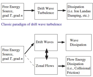
In magnetically confined plasmas, the role of turbulence is also understood as a way to dis-sipate the energy from the larger scales to the small ones, in form of micro-instabilities. The turbulent regime is characterized by small fluctuations in the mean plasma parameters, such as pressure, electric field and temperature. In this case, the energy is passed from larger scales to small ones, through cascades, where the energy can be finally released in the form of heat, as schematized in figure 4.1.

Figura 4.1: Archetype of dissipation pathways within turbulent framework[P H Diamond1 et. al.]

In order to describe themodus operandi of turbulent behavior, we are going to work in the framework of the Gyrokinetic description of the plasma. In this scheme, the fluctuations present in the parameters of interest can be analyzed in more detail, and it opens, also, a path for a redu-ced numerical solution of the whole process, which is interesting if one thinks about the use of computational resources as a tool for the description of the phenomena.

4.2 GYROKINETIC APPROACH