Sustainability of Brazilian public debt: analysis of a possible structural break in the recent period

Ensaios Econômicos

Sustainability of Brazilian public debt:

analy-sis of a possible structural break in the recent

period

Eduardo Lima Campos, Rubens Penha Cysne

Os artigos publicados são de inteira responsabilidade de seus autores. As

opiniões neles emitidas não exprimem, necessariamente, o ponto de vista da

Fundação Getulio Vargas.

EPGE Escola Brasileira de Economia e Finanças Diretor Geral: Rubens Penha Cysne

Vice-Diretor: Aloisio Araujo

Coordenador de Regulação Institucional: Luis Henrique Bertolino Braido

Coordenadores de Graduação: Luis Henrique Bertolino Braido & André Arruda Villela Coordenadores de Pós-graduação Acadêmica: Humberto Moreira & Lucas Jóver Maestri Coordenadores do Mestrado Profissional em Economia e Finanças: Ricardo de Oliveira Cavalcanti & Joísa Campanher Dutra

Lima Campos, Eduardo

Sustainability of Brazilian public debt: analysis of a possible structural break in the recent period/

Eduardo Lima Campos, Rubens Penha Cysne – Rio de Janeiro : FGV,EPGE, 2019

25p. - (Ensaios Econômicos; 806) Inclui bibliografia.

Sustainability of Brazilian public debt: analysis of a possible structural break in the recent period

Eduardo Lima Campos and Rubens Penha Cysne

Abstract

Campos and Cysne (2019a) use the multicointegration method to analyze the behavior of Brazilian public debt between 1997 and 2018. The authors observe, in this previous work, the necessity of evaluating the existence of a structural break along the sample, corroborating assumptions originated from the political cycle. This paper evaluates that possibility, and identifies its possible effects on the sustainability of the public debt. The conclusion regarding the unsustainability of the debt/GDP ratio is confirmed. But here we are able to identify the precise date as of which the debt trajectory becomes unsustainable. Using a technique which allows for a structural break has two additional advantages with regard to Campos and Cysne (2019a). First, it enables the comparison of the models before and after the break. Second, to a certain extent, it includes the possibility of comparisons with previous empirical works based on variable-coefficient methodologies [e.g. Campos and Cysne (2019b)].

Key words: public debt, sustainability, multicointegration, structural breaks.

1. Introduction1

Leachman et al. (2005) suggest using the multicointegration technique to evaluate the sustainability of public debt, arguing that this methodology corrects limitations of the traditional cointegration-based approach, investigating not only the long-term relationship between revenues and expenditures, but also between these variables and the stock of net debt2.

Campos and Cysne (2019a) use this technique to analyze the behavior of Brazilian public debt between 1997 and 2018. The authors conclude that, considering cumulative revenue as a dependent variable, the debt was weakly sustainable – in the sense established by Quintos (1995) – over the study period, which means that, although an equilibrium relationship is verified between revenues and expenditures, these variables do not react in sufficient magnitude to variations in the debt. Conversely, when cumulative spending is considered as a dependent variable, the paper’s conclusion is that the debt was unsustainable in the study period.

Also with reference to Campos and Cysne (2019a), an analysis of the residuals of the estimated models paves the way to investigating whether the debt can be kept sustainable only up to a certain period. It is worth highlighting that this would be aligned with other studies using recent data from the Brazilian economy, which indicate a transition of the debt towards an unsustainable trajectory over recent years (see, for example, Campos and Cysne, 2019b).

Some papers seek to overcome this adversity by using cointegration tests with a structural break (Gregory and Hamsen, 1996), or Markovian transition models (see, for example, Mendonça et al. (2009) and Simonassi et al. (2007, 2013)). However, the first approach is subject to criticism from Bohn (2007), while the second, besides not allowing for the exact moments at which structural breaks occur to be estimated, does not enable clear comparisons to be established between the running of a fiscal policy before and after regime changes.

This paper incorporates structural breaks into the multicointegration models, following Haldrup (1994) and Engsted et al. (1999), which enables a possible regime change in the reaction of revenues and/or expenditures to variations in the stock of debt to be investigated. The technique proposed by Berenguer-Rico and Carrion-I-Silvestre (2011) is also incorporated to estimate the moment at which the transition occurs, making it possible to identify when the transition took place, as well as enabling possible differences in the running of fiscal policy before and after the break to be evaluated and interpreted.

The conclusion of this work is that, up until mid-2014, Brazilian fiscal policy did in fact present weak sustainability, corroborating the results of Campos and Cysne (2019a).

1 _{We thank Carlos Henrique Dias for his research assistance.}

2 _{The variables deficit and debt, when not otherwise specified, are always to be considered here as a}

Yet, from May of 2014 onwards, a transition towards an unsustainable regime is identified, caused by the increase in spending at rising rates, without a sufficient offsetting of revenues.

2. Objectives

This paper uses the multicointegration method with an endogenous structural break to investigate: 1) whether, over the study period considered in Campos and Cysne (2019a), there was a structural break; 2) whether, at the time of this break, the characteristics of Brazilian fiscal policy changed – becoming, for example, unsustainable; 3) if so, whether it was revenues, expenditures, or both, that caused this transition; and 4) whether there are differences in the running of fiscal policy before and after this break, and if so, these will be quantified.

An alternative approach to the sustainability issue is based on the fiscal reaction function, which relates the primary surplus with variations in the level of the debt/GDP ratio (Bohn, 2008). Campos and Cysne (2019b) apply this approach to data from the Brazilian consolidated public sector, using a method that enables the fiscal reaction parameter to vary over time. In this paper, this method was also considered and applied to central government data, leading to similar results to those obtained in Campos and Cysne (2019b), which suggests a recent transition of Brazilian fiscal policy towards an unsustainable regime.

3. Data analysis

The data series used (all expressed as a percentage of 12-month cumulative nominal GDP) reproduce those also used in Campos and Cysne (2019a). For the central government, we have: 𝑦_𝑡 = revenue, 𝑥_𝑡= total spending (that is, including debt interest payments), and 𝑏_𝑡 = stock of debt, with a monthly frequency, from December of 1997 to June of 2018. These variables were all obtained from the Brazilian Central Bank and National Treasury websites.

Based on the data analysis, the suggestion of a possible structural break in the recent period derives from Figures 5.1 and 6.1 of Campos and Cysne (2019a), reproduced below:

[Figure 3.1 near here] [Figure 3.2 near here]

Both time series show a change in inclination at the end of the study period. In figure 3.2, in particular, which represents the model that presents spending as a dependent variable, this change becomes more evident. This indicates a possible structural break. The main consequence of this is that the results of the unit root test in the residuals may alter, thus affecting the conclusions of the previous paper regarding sustainability of the debt.

Therefore, it warrants investigating whether there was, in fact, a structural break at the end of the sample. And, if there was, did this break cause a transition in fiscal policy towards unsustainability? In this case, so that the paper can guide the running of fiscal policy, it needs to be identified whether this transition was due to the fall in revenues, to the increase in spending, or to the joint effect of these variables. For this purpose, separate models are used for revenues and expenditures.

4. Multicointegration model with a structural break

Campos and Cysne (2019a) use the multicointegration method (Granger and Lee, 1989) to investigate the possible existence of a long-term relationship between cumulative revenues and cumulative expenditures, 𝑌𝑡 = ∑𝑡𝑗=1𝑦𝑗 and 𝑋𝑡 = ∑𝑡𝑗=1𝑥𝑗, and the stock of public debt/GDP ratio, 𝑏_𝑡, using quarterly data series from the period situated between 1997 and 2018. Leachman et al. (2005) and Engsted et al. (2007) demonstrated that if this relationship is verified, the debt is sustainable.

This paper investigates the presence of a possible structural break in the relationship between 𝑌𝑡, 𝑋𝑡, and 𝑏𝑡. If it is identified, this break needs to be incorporated into the conventional multicointegration models; otherwise the results generated may be inconclusive and/or lead to erroneous conclusions. In particular, Berrenguer and Rico (2011) argued that the multicointegration tests have little power in the presence of a structural break; that is, they tend to indicate the absence of a multicointegration relationship between the time series considered.

Two models were considered, called 1 and 2 here, considering cumulative revenue and cumulative spending as dependent variables, respectively, and incorporating a structural break into moment 𝑇_𝑏 (to be estimated). The specification of model 1 is presented below:

𝑌_𝑡 = 𝛽₀₀+ 𝛽₀₁𝑡 + 𝛽₀₂1(𝑡 > 𝑇_𝑏) + 𝛽₀₃(𝑡 − 𝑇_𝑏)1(𝑡 > 𝑇_𝑏) + 𝛼𝑡2_{+ 𝛽} 11𝑏𝑡

+ 𝛽12𝑏𝑡1(𝑡 > 𝑇𝑏) + 𝛽21𝑋𝑡+ 𝛽22𝑋𝑡1(𝑡 > 𝑇𝑏) +𝑡 _(4.1)

in which 𝑡 and 𝑡2 are the terms of the linear and quadratic trend, respectively; 𝑇_𝑏 represents the break point (to be estimated); 𝛽₀₂ and 𝛽₀₃ capture changes in the level and in the trend, respectively; 𝛽₁₂ and 𝛽₂₂ represent a change in the effect (due to the break) of the 𝑏𝑡 and 𝑋𝑡 variables over cumulative revenue 𝑌𝑡; and 𝑡 is the error term of the model.

Model 2, which considers cumulative spending as a dependent variable, is described below:

𝑋_𝑡 = 𝛽₀₀+ 𝛽₀₁𝑡 + 𝛽₀₂1(𝑡 > 𝑇_𝑏) + 𝛽03(𝑡 − 𝑇𝑏)1(𝑡 > 𝑇𝑏) + 𝛼𝑡2+ 𝛽11𝑏𝑡 + 𝛽₁₂𝑏_𝑡1(𝑡 > 𝑇_𝑏) + 𝛽₂₁𝑌_𝑡+ 𝛽₂₂𝑌_𝑡1(𝑡 > 𝑇_𝑏) +_𝑡

(4.2)

The approach presented here is based on Berenguer-Rico and Carrion-I Silvestre (2011), which enables breaks both in the deterministic terms, and in the coefficients of the variables involved, to be investigated, as well as estimating the exact moment at which the regime transition occurred.

To evaluate the stationarity of the residuals 𝜀̂_𝑡 derived from the estimation of models (4.1) or (4.2), the conventional unit root test is initially applied; that is, the following equation is estimated:

∆𝜀̂𝑡= 𝛿𝜀̂𝑡−1+ ∑ 𝜙𝑗∆𝜀̂𝑡−𝑗+ 𝜂𝑡 𝑃

𝐽=0

(4.3)

Next, the hypothesis H0: 𝛿 = 0 is tested. This procedure produces a sequence of t statistics for each possible break point 𝜆 ∈ Λ3. Denoting the t statistic associated with each possible value of the break fraction 𝜆 as 𝑡_𝛿(𝜆), the infimum of the sequence is denoted as:

𝑡_𝛿∗ _{= inf 𝑡}

𝛿 (𝜆) (4.4)

Finally, the statistic in (4.4) is used to evaluate the existence of multicointegration with a structural break. The hypotheses of the test are: H0: there is no multicointegration relationship, that is, the residuals are not I(0) versus H1: ̂_𝑡 ~ I(0), there is a multicointegration relationship and in this case, as according to Leachman et al. (2005), fiscal policy can be considered sustainable. The asymptotic distribution of 𝑡_𝛿∗ depends on the specifications adopted in equations (4.1)-(4.2), particularly on the number of regressors I(1) and I(2) included in each equation.

Regarding the detection of 𝑇𝑏 (date associated with 𝑡𝛿∗), the criterion used is to minimize the sum of the squares of the residuals from the estimation of (4.1)-(4.2), for 𝜆(0,1). To make the analysis robust to the generating process, the following specifications were considered:

[Table 4.1 near here]

5. Results – revenues as a dependent variable (model 1)

3 The date of the break point is expressed as 𝑇

𝑏= [𝜆𝑛], where n is the sample size, and 𝜆, is the break

This section will follow model 1, presented in equation (4.1).

Below are the results of the test for determining the break point for each one of the specifications presented in table 4.1. As the date of the break point 𝑇_𝑏 is endogenous, equation (4.1) was estimated for each possible structural break throughout the sample. The values of the test statistic in (4.3), and the respective critical values of the Berenguer-Rico and Carrion-I-Silvestre (2011) test, are presented in table 5.1 below.

[Table 5.1 near here]

The initial results indicate the existence of a significant structural break. However, they are not conclusive in relation to the moment at which this break occurs. Thus, a more detailed analysis of the estimates provided by each model and of statistics to evaluate the quality of the adjustments is needed to obtain a more precise diagnosis.

Table 5.2 below presents the estimated coefficients for model 1, whose equation is repeated below for convenience: 𝑌_𝑡 = 𝛽₀₀+ 𝛽₀₁𝑡 + 𝛽₀₂1(𝑡 > 𝑇_𝑏) + 𝛽₀₃(𝑡 − 𝑇_𝑏)1(𝑡 > 𝑇_𝑏) + 𝛼𝑡2 _{+ 𝛽}

11𝑏𝑡+ 𝛽12𝑏𝑡1(𝑡 > 𝑇𝑏) + 𝛽21𝑋𝑡+ 𝛽22𝑋𝑡1(𝑡 > 𝑇𝑏) +𝑡.

[Table 5.2 near here]

The coefficients 𝛽₀₁ and 𝛽₀₃ reveal a change in the level and in the trend of the time series after the structural break, for all the models. It is also observed that the quadratic trend was not significant (at the 0.05 level) in model [B], and thus that the results of this model will not be of much relevance, since the only difference for model [A] is precisely the t2 _term.

The estimates of 𝛽₂₁ was significant and stable and have a magnitude of around 0.4 (less than one, as expected), for all the models. Over again, the only exception was the model [B] (with a little lower estimated value of 𝛽₂₁). There is, therefore, evidence that the growth in cumulative revenue was significantly lower than that of cumulative spending, before the structural break. After the break, the estimates of 𝛽22 in models [C] and [E] indicate a significant reduction (at the 0.05 level) in the spending coefficient (𝛽21+𝛽22). That is, after the structural break, the low growth in revenue in relation to spending not only persists, but is accentuated. This may compromise the strength of the relationship between the variables and even the weak sustainability indicated by model 1 (section 5.1), which does not consider a structural break.

Finally, the estimate of coefficient 𝛽₁₁, which represents the reaction of cumulative revenue to the stock of debt, presents positive and statistically significant values for all the models. This indicates an increase in the variation of cumulative revenue in response

to increases in the level of debt before the structural break, which is consistent with the empirical evaluation of Brazilian fiscal policy in the period: sustainability of the fiscal trajectory based on the endogenous reaction of revenues, given an increase in expenditures. After the break, however, the negative point estimates of 𝛽₁₂ in models [D] and [E] indicate that this reaction was attenuated, such that it possibly compromised the sustainability of fiscal policy.

In relation to the effects of the structural break over the running of fiscal policy, it is of fundamental importance to explicitly compare the coefficients of variables 𝑏_𝑡 and 𝑋_𝑡 before and after the respective estimated break, with regards to the sign, magnitude, and significance4_{. The final results (point estimates and t statistics) are presented in table 5.3} below.

[Table 5.3 near here]

Before the structural break, there is evidence of an equilibrium relationship between revenue and spending, but not between both cumulative revenue and cumulative spending and the stock of debt, which indicates weak sustainability of fiscal policy before the structural break. A strong positive and significant reaction of revenue to variations in the debt is also verified, which may indicate that the absence of strong sustainability indicated in Campos and Cysne (2019a) is, in fact, due to the disequilibrium of the last years of the study period, which reinforces the need to consider a structural break. After the break, there are indications that the relationship between revenues and expenditures altered, since the estimate of the post-break coefficients (𝛽₂₁+𝛽₂₂) was approximately 0.1 (= 0.4261-0.3264, in model [1C], and 0.4583-0.3595, in model [1E]).

The multicointegration tests, that is, the Dickey and Pantula tests for 2 unit roots, considering a structural break, to the residuals of models [1A]-[1E], are presented below:

[Table 5.4 near here]

4 _{In the case of the significance, there is an additional question to be overcome: the standard errors of the}

coefficients after the break (given by a sum of coefficients) cannot be obtained based on the simple sum of the variances of the coefficients involved. The correlation between the coefficients must be considered. Thus, based on the estimated variance-covariance matrices, the standard errors of each effect were calculated.

It can be noted that, in all the cases, the results indicate weak sustainability, which is the same conclusion as Campos and Cysne (2019a). Only model [1B] leads to a different conclusion, possibly due to the presence of a quadratic trend. Yet, the quadratic trend term is not significant (table 5.2), which leads us to ignore this specific result and, thus, conclude that the series presents only first level cointegration, even when a structural break is incorporated, maintaining the evidence of weak sustainability of Brazilian fiscal policy over the study period.

Finally, a comparison was made of the models estimated in table 5.2. For this, information criteria were used, since the models have different quantities of parameters, and comparing them using some adjustment statistic that did not penalize the number of parameters (such as the sum of the squares of the residuals) could lead to an overparametrized model. The information criteria adopted were those of Akaike (AIC) and Schwarz (SBC), which are most commonly used in the time series literature. The results are presented in table 5.5, below.

[Table 5.5 near here]

The AIC criteria led to model [1E]. The SBC criterion, which is more parsimonious, led to model [1C]. In this paper, model [1E] was chosen, for the following reasons: 1) the only parameter that differentiates these models is 𝛽₁₂, whose estimate was not only significant in model [1E], but its interpretation is of fundamental importance here; 2) the difference between the SBCs in models [1C] and [1E] is in the order of 10-5, while the difference between the respective AICs is around 0.007; and 3) the sensitivity of all the other coefficients to the presence or not of the 𝛽12 coefficient is very small, even maintaining all the corresponding interpretations when alternating between these models.

Finally, note that, according to table 5.1, both model [1C] and model [1E] indicate the same break point: May of 2014. Thus, the analysis leads to the robust conclusion that this is the break point for the model in which the dependent variable is public revenue. The equation of the specification chosen for model 1 is presented below, with its respective coefficients and t statistic, with the break-down before and after the structural break:

Before the break:

𝑌_𝑡 = −0.1360 + 0.0347𝑡 + 0.0756𝑏_𝑡+ 0.4583𝑋_𝑡

(5.1)

After the break:

𝑌_𝑡 = −0.0776 − 0.0047𝑡 + 0.0365𝑏_𝑡+ 0.0988𝑋_𝑡

(5.2)

(-2.8522) (-1.7885) (1.5708) (2.0226)

The non-significance of the effects after the structural break indicates that the weak sustainability may have been kept, that is, there is no multicointegration after the break. The analysis of the graph of the residuals of model [1E], comparing its trajectory before and after the structural break in May of 2014, is useful in this process. The results are presented in figure 5.1:

[Figure 5.1 near here]

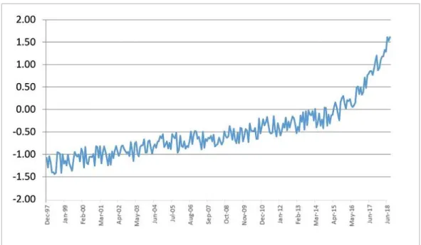
Comparing with the residuals of the model for revenues, with a break, estimated in Campos and Cysne (2019a) (see figure 3.1 here), there is evidence of a structural break in May of 2014.

The graph of the residuals before and after the break for model [1E] indicates that, from incorporating the structural break, the model for revenues duly accommodated the break, thus indicating that this series does not appear to have altered its trajectory significantly after the possible transition. The result of the unit root test for the complete series, which indicated first order integration, does not alter when the break is incorporated, which remains with trajectory I(1). Thus, the revenues break after the structural break, in isolation, does not appear to have been enough to have made Brazilian fiscal policy unsustainable. It is also worth highlighting that the results obtained in this section are more reliable, since the Dickey and Pantula test has little power in the presence of a structural break, if it is not recognized and incorporated into the estimation.

Thus, according to model [1E], it is concluded that Brazilian fiscal policy remains on a trajectory of weak sustainability, despite the decreasing reactivity of revenues given the increase in expenditures. Yet, the specification considered treats cumulative revenue as a dependent variable, and it thus warrants investigating whether the inversion of cumulative revenues and cumulative expenditures in this model leads to different conclusions. This is the object of section 6.

6. Results – spending as a dependent variable (model 2)

This section will follow the model from equation (4.2), which we call model 2.

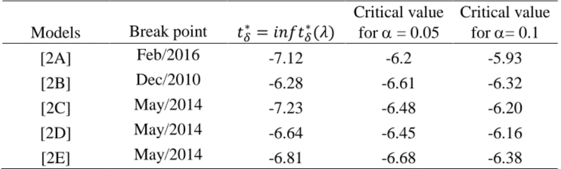
The values of the test statistic in (5.4), and the respective critical values of the Berenguer-Rico and Carrion-I-Silvestre (2011) test, are presented in table 6.1, below.

[Table 6.1 near here]

In the case of the spending model, it is concluded that there is a clear indication that the structural break occurs in May of 2014, since, of the four models that indicated the significance of the structural break (the only exception was model [2B]), three point to this date. Nonetheless, a detailed analysis of the estimates provided by each model and of statistics for evaluating the quality of the adjustments is important to complement and formalize the analysis.

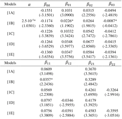
Table 6.2 below presents the estimated coefficients for model 2, whose equation (4.2) is repeated below for convenience: 𝑋𝑡 = 𝛽00+ 𝛽01𝑡 + 𝛽021(𝑡 > 𝑇𝑏) + 𝛽03(𝑡 − 𝑇𝑏)1(𝑡 > 𝑇𝑏) + 𝛼𝑡2 + 𝛽11𝑏𝑡+ 𝛽12𝑏𝑡1(𝑡 > 𝑇𝑏) + 𝛽21𝑌𝑡+ 𝛽22𝑌𝑡1(𝑡 > 𝑇𝑏) +𝑡:

[Table 6.2 near here]

The coefficients 𝛽01 and 𝛽03 reveal a change in the level and in the trend of the series after the structural break, for all the models, except for model [2B], in which the deterministic trend before the break is non-significant at the 0.05 level. It is observed, however, that the quadratic trend was non-significant (at the 0.05 level) in model [2B], and therefore the results of this model will be ignored, following the procedure adopted in model 1.

The 𝛽21 estimate was significant and presented higher values than 1, which were stable, being of a magnitude of around 1.25 for all the models. There is, therefore, evidence that the growth in cumulative spending significantly exceeded that of cumulative revenue, before the structural break. After the break, the 𝛽22 estimates in models [2C] and [2E] indicate an enhancement of this effect on the revenue coefficient (𝛽21+𝛽22). That is, after the structural break, the growth in spending in relation to revenue was accentuated.

Finally, the estimate of the 𝛽11 coefficient, which represents the reaction of cumulative spending to the stock of debt, presents positive and statistically significant values for all the models. This indicates a reaction of the expenditures series to the increase in public debt, however contrary to expected, since spending increases instead of decreasing. Therefore, previously the break, the weak sustainability of public debt was exclusively due to the accumulation of revenues, whose measure was sufficient to compensate for the growth in expenditures.

After the break, however, the positive estimates of 𝛽12 in models [2C] and [2E] indicate that the increase in debt in relation to revenue was enhanced, so as to possibly compromise the sustainability of fiscal policy.

In relation to the effects of the structural break over the running of fiscal policy, it is important to explicitly compare the coefficients of the 𝑏_𝑡 and 𝑌_𝑡 variables before and after the break, with regards to the sign, magnitude, and significance, as was done for the model in section 5. The results (point estimates and t statistics) are presented in table 6.3 below.

[Table 6.3 near here]

Before the structural break, there are indications of an equilibrium relationship between revenue and spending, but not between both cumulative revenue and cumulative spending and the stock of debt, which indicates weak sustainability of fiscal policy before the structural break. A strong positive and significant reaction of spending to variations in the debt is also verified, however with the opposite sign to what would be desirable, which may indicate that the absence of strong sustainability indicated by the models in section 6 was, in fact, due to the disequilibrium in the last years of the sample. This fact reinforces the need to consider a structural break. In fact, after the break, there are indications that the discrepancy between the rate of accumulation of revenues and expenditures was accentuated, since the estimate of the post-break coefficient (𝛽21+𝛽22) was approximately 1.32 (>1.05) in model [4C], and 1.35 (>1.07) in model [2E].

The multicointegration tests, that is, the Dickey and Pantula tests for 2 unit roots, considering a structural break, to the residuals of models [2A]-[2E], are presented below:

[Table 6.4 near here]

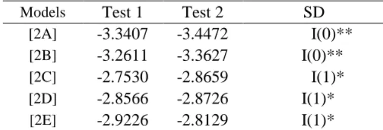
|It can be noted that only in the case of the last 3 specifications do the results indicate weak sustainability, in this case maintaining the conclusion of the models with a structural break estimated in Campos and Cysne (2019a).

Finally, a comparison was made of the models estimated in table 6.2. For this, the Akaike (AIC) and Schwarz (SBC) information criteria were used, as in section 5. The results are presented in table 6.5, below.

The AIC criterion led to model [2E]. The SBC criterion, which is more parsimonious, led to model [2C]. As in section 5, model [2E] was chosen, for the following reasons: 1) the only parameter that differentiates these models is 𝛽12, whose estimate was not only significant in model [2E], but its interpretation is of fundamental importance here; 2) the difference between the SBCs in models [2C] and [2E] is much smaller than the difference between the respective AICs; and 3) the sensitivity of all the other coefficients of these models to the presence or not of the 𝛽12 coefficient is very small, even maintaining all the corresponding interpretations when alternating between these models. In light of this, model [2E] was chosen.

Finally, note that, according to table 6.1, both model [2C] and model [2E] indicate the same break point: May of 2014. Thus, the analysis enables it to be concluded that this is the break point for the model in which the dependent variable is public spending.

The equation of the specification chosen for model 2 is presented below, with its respective coefficients, and with the break-down before and after the structural break: Before the break:

𝑌_𝑡 = 0.1901 + 0.1127𝑡 + 0.0184𝑏_𝑡+ 1.0784𝑋_𝑡

(6.1)

(3.5527) (3.7789) (3.9624) (2.6981)

After the break:

𝑌_𝑡 = 0.2345 + 0.3301𝑡 + 0.0491𝑏_𝑡+ 1.3541𝑋_𝑡

(6.2)

(2.8522) (3.9885) (5.2672) (3.3431)

The significance of the effects after the structural break indicates that the weak sustainability may have been compromised, that is, after the break there is no first level cointegration. Contributing to this suspicion is the increase in the discrepancy between the growth in expenditures and the reaction of revenues, indicated in the comparison of equations 6.1 and 6.2. To investigate this point, the residuals before and after the break for model [1E] are presented below:

It is observed that the structural break was duly accommodated by the residuals. Comparing with the residuals of figure 3.2 (model for expenditures, without structural break), it becomes evident that there was in fact a structural break in May of 2014. Also, the method indicates that Brazilian fiscal policy became unsustainable from May of 2014 onwards, when we consider the model with public spending as a dependent variable.

One explanation for the result of this section is that, given the decreasing reaction of revenues, the uncontrolled increase in expenditures, with acceleration both in primary spending and in that related to servicing the debt itself, led to a regime change. And not even the implementation of new expenditure controls enacted in 2016 (EC 95/2016) was enough to regain the sustainability of fiscal policy, at least based on the parameters in effect up to the conclusion of this paper (June of 2018).

It is worth highlighting that total expenditures (primary plus interest) are being considered, which indicates that the absence of sustainability identified after the break may be essentially due to the debt service charges, that is, not only due to the growth in the debt, but also the interest rate, which varied quite a lot precisely over this specific period.

7. Fiscal reaction function for the central government

A fiscal reaction function represents how the government’s primary surplus 𝑠_𝑡 responds to variations in the debt 𝑏_𝑡, both measured as a percentage of GDP (Bohn, 1998). The coefficient that relates these two variables is called the fiscal reaction function, which we will denote as . In general, a fiscal reaction function can be specified as follows:

st = c +bt−1+ other control variables + error. (7.1) “Other control variables” can include the output gap, the interest rate, the risk premium, lags in the dependent variable 𝑠_𝑡, and any other relevant variable.

An important result associated with the fiscal reaction function is that, as shown in section 2.2 of the abovementioned article, if  is greater than the difference between the real interest rate and the GDP growth rate, it can be concluded that the public debt is sustainable in the long run.

Campos and Cysne (2019b) estimate a fiscal reaction function for the 2003-2016 period, using monthly data from the consolidated public sector and considering the time-variant coefficients of the function. The authors conclude that the debt became unsustainable from 2014 onwards.

In this section, the fiscal reaction function is re-estimated, this time using the central government data used in this paper. The estimation method adopted was the Kalman

Filter. The aim is to analyze whether the fiscal reaction function approach leads to similar conclusions.

Thus, if st is the primary surplus/GDP ratio, bt is the debt/GDP ratio, h_t is the output gap, and PR_t is the risk premium (EMBI) in month t5, the fiscal reaction function estimated for the month of June of 2018 is:

st = 0.0151 + 0.8722st−1− 0.0019bt−1+ 0.0948 ht−1− 0.0280PRt

(7.2) (2.2108) (5.1203) (-4.7861) (2.9746) (-3.1872)

It should be observed, in particular, that the fiscal reaction in June of 2018 is negative, which reflects the fact that, given the increase in the debt, the primary surplus not only ceases to react sufficiently to compensate for the increase, but it decreases. As we have already seen throughout this paper, this behavior is due to the accentuated growth of expenditures over the last years.

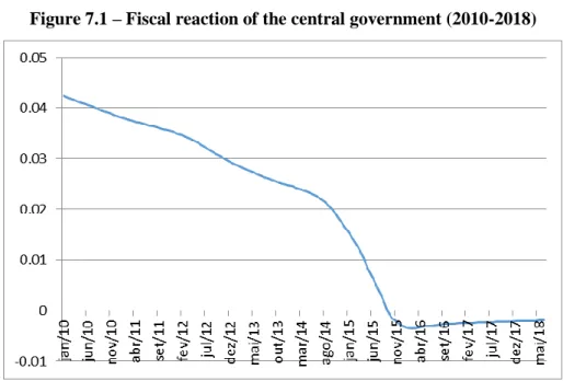
For the purposes of analyzing long-term sustainability, it is important to observe the behavior of the fiscal reaction coefficient over time, presented in figure 7.1:

[Figure 7.1 near here]

As the main interest is in the last years of the study period, the graph was drawn up considering only a sub-sample, from January of 2010 to June of 2018 (although the whole sample was used for the estimation). An initially positive fiscal reaction coefficient is observed, which gradually loses strength. This result is explained by the fall in the debt/GDP ratio, which only adopts a rising trajectory from 2015 onwards. An interesting aspect of the graph in figure 7.1 is that it is possible to identify an inflection point in May of 2014, precisely the break point that was estimated in this paper. This means that, from this month onwards, an intensification of the fall in the fiscal reaction is observed, which may be explained by the increase in expenditures that begins precisely in that month. It should be observed that this behavior was due, in part, to the successive increases in interest rates in the period, since total expenditures are being considered, and not only primary ones.

Finally, in October of 2015, an inversion of the sign of the estimated fiscal reaction is noted. This moment corresponds to the inversion of the trajectory of the debt/GDP ratio, which adopts a rising trajectory. It should be observed that this inversion of sign also occurs when data from the consolidated public sector are used, however in November of 2017 (see Campos and Cysne (2019c)).

In the last two years of the sample, it is verified that the fiscal reaction remains negative. However, from February of 2016 onwards, when it reaches its minimum point, it starts to grow dramatically over the year, which may be explained based on the fall in expenditures verified over the period, without an offsetting of revenues, which, on the contrary, decreased in that year.

From the last quarter of 2016 onwards, the fiscal reaction kept its rising trajectory. However, it tends to stabilize at a value quite close to zero that is statistically non-significant at the usual levels, according to the estimate in (7.2). It is therefore concluded that the fiscal reaction is, from a statistical perspective, inexistent over the last months of the sample.

Another important conclusion is that, in May of 2014, the fiscal reaction is worth approximately 0.025, which is an insufficient value to guarantee the sustainability of the debt. This reiterates the fact that fiscal policy is unsustainable from this date onwards. However, an analysis of the evolution of the difference between the interest rates and GDP growth and the estimated fiscal reaction shows that, according to this methodology, fiscal policy becomes unsustainable from May of 2014 onwards.

The results obtained with the fiscal reaction function are consistent with the conclusions of this paper, obtained via multicointegration, that there was in fact a gradual transition of Brazilian fiscal policy, over recent years, towards an unsustainable trajectory.

One caveat: the fiscal reaction function represents the reaction of the primary surplus to variations in the public debt, in a symmetrical way, that is, without specifying whether this reaction is due to revenues, to expenditures, or to both. The method adopted in this paper, on the other hand, enables it to be identified whether the reaction of fiscal policy (or its absence) occurs through variations in revenues or in expenditures. It also involves a more complex equilibrium relationship and a statistical method for estimating an endogenous structural break, which reiterates that the break did in fact occur in May of 2014.

8. Conclusions

This paper investigated the existence of a structural break in the multicointegration models that relate revenues and expenditures accumulated over time and the stock of debt/GDP ratio, estimated in Campos and Cysne (2019b). According to Leachman et al. (2005), this technique enables conclusions to be made regarding the sustainability or not of fiscal policy, unlike the conventional unit root and cointegration tests.

The structural break was treated as endogenous, and estimated considering various specifications of models, which provided the analysis with robustness. Using a method proposed by Berenguer-Rico and Carrion-I-Silvestre (2011), the conclusion was reached that a structural break occurred in May of 2014. The next step was to identify which factors caused this break.

Incorporating the structural break and using revenue as a dependent variable, we conclude that Brazilian fiscal policy was weakly sustainable over the whole study period, despite the decreasing reactivity of revenues to the increase in expenditures. On the other hand, when we consider the model with spending as a dependent variable, indications emerge that Brazilian fiscal policy became unsustainable from May of 2014 onwards. This result adds an important insight not present in Campos and Cysne (2019a), the identification of the specific date as of which the debt trajectory is not sustainable. One possible explanation for this result was the sharp increase in total expenditures, with an insufficient offsetting of revenues – responsible up to then for guaranteeing the fiscal reaction – in the period.

This paper corroborates the conclusions of Campos and Cysne (2019b), which were based on the fiscal reaction function. That is, a gradual transition is characterized of Brazilian fiscal policy in recent years, towards an unsustainable trajectory. However, this comes with an additional advantage. The fiscal reaction only represents the reaction of the primary surplus to variations in the debt, and does not enable it to be verified whether this reaction is due to revenues or to expenditures. On the other hand, the method adopted here enables it to be identified whether the fiscal policy reaction (or its absence) occurs through variations in revenues or in expenditures (or both). It also involves a more complex econometric equilibrium relationship and the possibility of estimating the exact moment at which an endogenous structural break occurs.

In summary, the methodology used in this paper enables the suggestion that, given the decreasing reaction of revenues, which thus becomes insufficient, the uncontrolled increase in expenditures – with acceleration both in primary expenditures and in those related to servicing the debt itself – led to a regime change in public debt towards an unsustainable trajectory. And not even the implementation of new expenditure controls enacted in 2016 (EC 95/2016) was enough to regain the sustainability of fiscal policy. Not even in its weak form, at least based on the parameters in effect up until the conclusion of this paper, that is, using fiscal variables observed up to June of 2018.

Bibliography

Banco Central do Brasil. (2016). Dívida líquida e bruta do governo geral. Retrieved from Sistema Gerenciador de Séries Temporais: https://www3.bcb.gov.br/sgspub

Banco Central do Brasil. (2016). Relatório de Indicadores Fiscais de junho/2016. Retrieved from

https://www.bcb.gov.br/conteudo/home-ptbr/FAQs/FAQ%2004-Indicadores%20Fiscais.pdf

Berenguer-Rico, V. & J.L. Carrion-I-Silvestre. (2011). “Regime Shifts in Stock-Flow I(2)-I(1) Systems: The Case of US Fiscal Sustainability. Journal of Applied Econometrics, 26(2), 298-321.

Bohn, H. (1998). The Behavior of U.S. Public Debt and Deficits. The Quarterly Journal of Economics, 113(3), 949-963.

Bohn, H. (2007). Are stationarity and cointegration restrictions really necessary for the intertemporal budget constraint? Journal of monetary Economics, 54(7), 1837-1847. Bohn, H. (2008). The sustainability of fiscal policy in the United States. Sustainability of public

debt, 15-49.

Campos, E. L., & Cysne, R. P. (2019a). Sustainability of the Brazilian Public Debt - an Analysis Using Multicointegration [Working Paper]. Ensaios Econômicos, Escola Brasileira de Economia e Finanças da FGV (https://epge.fgv.br/users/rubens/working-papers). Campos, E. L., & Cysne, R. P. (2019b). A Time-Varying Fiscal Reaction Function for Brazil.

Estudos Econômicos, 49(1), p. 5-38.

Campos, E. L., & Cysne, R. P. (2019c). An alert on the recent fall of the fiscal reaction in Brazil [Working Paper Nº 799]. Ensaios Econômicos, Escola Brasileira de Economia e

Finanças da FGV (https://epge.fgv.br/users/rubens/working-papers).

Dickey, D. A., & Pantula, S. G. (1987). Determining the order of differencing in autoregressive processes. Journal of Business & Economic Statistics, 5(4), 455-461.

Engsted, T., & N. Haldrup. (1999). Multicointegration in Stock-Flow Models. Oxford Bulletin of Economics and Statistics, 61(2), 237-254.

Engsted, T., & Tanggaard, C. (2007). The comovement of US and German bond markets. International Review of Financial Analysis, 16, 172-182.

Granger, C. W., & Lee, T. H. (1989). Investigation of production, sales and inventory relationships using multicointegration and non‐symmetric error correction models. Journal of applied econometrics, 4(S1), S145-S159.

Gregory, A. W., & Hansen, B. E. (1996). Residual-based tests for cointegration in models with regime shifts. Journal of econometrics, 70(1), 99-126.

Haldrup, N. (1994). The asymptotics of single-equation cointegration regressions with I (1) and I (2) variables. Journal of Econometrics, 63(1), 153-181.

IBGE. (2016). Retrieved from Séries Históricas e Estatísticas: https://seriesestatisticas.ibge.gov.br/

Instituto Brasileiro de Economia. (n.d.). Monitor do PIB/FGV. Retrieved from Portal IBRE: http://portalibre.fgv.br/main.jsp?lumChannelId=8A7C82C5593FD36B015D5C57E7571 5CA

Kalman, R. E. (1960). A New Approach to Linear Filtering and Prediction Problems. Journal of Basic Engineering, 82(1), 35-45.

Kalman, R. E., & Bucy, R. S. (1961). New Results in Linear Filtering and Prediction Theory. Journal of Basic Enginnering, 93(1), 85-108.

Leachman, L., A. Bester , G. Rosas, & P. Lange. (2005). Multicointegration and Sustainability of Fiscal Practices. Economic Inquiry, 43(2), 454-466.

Mendonça, M. J., Santos, C. H., & Sachsida, A. (2009). Revisitando a função de reação fiscal no Brasil pós-Real: uma abordagem de mudanças de regime. Estudos Econômicos, 39(4), 873-894.

Quintos, C. E. (1995). Sustainability of the deficit process with structural shifts. Journal of Business & Economic Statistics, 13(4), 409-417.

Simonassi, A. G. (2013). Reação fiscal sob mudanças estruturais e a solvência da economia brasileira. Mimeo. Ceará, Brazil: CAEN/UFC.

Simonassi, A. G., & Arraes, R. (2007). Função de resposta fiscal, múltiplas quebras estruturais e a sustentabilidade da dívida pública no Brasil. Recife-PE: XXXV Encontro da ANPEC.

Tesouro Nacional. (2016). Various works. Brazil.

Triches, D., & Bertussi, L. S. (2017). Multicointegração e sustentabilidade da política fiscal no Brasil com regime de quebras estruturais (1997-2015). Revista Brasileira de Economia, 71(3), 379-394.

Tronzano, M. (2014). Multicointegration and fiscal sustainability in India : evidence from standard and regime shifts models. Economia internazionale, 67(2), 263-291.

List of Figures:

Figure 3.1 - Residuals of model 1[B] – revenue as a dependent variable

Source: Campos and Cysne (2019a) (Figure 5.1).

Figure 3.2 - Residuals of model 2[B] – spending as a dependent variable, without considering the effect of structural breaks

Source: Campos and Cysne (2019a) (Figure 6.1).

Figure 5.1 – Residuals of model 1e – revenue as a dependent variable, with a structural break in May of 2014

Figure 6.1 – Residuals of model 2e – spending as a dependent variable, with a structural break in May of 2014

Figure 7.1 – Fiscal reaction of the central government (2010-2018)

List of Tables:

Table 4.1 – Alternative specifications of models 1 and 2 (equations 4.1 and 4.2).

Models Deterministic Part Stochastic Part [A]

[B] [C] [D] [E]

Table 5.1 – Test for determining the break point

Models Break point 𝑡_𝛿∗ = 𝑖𝑛𝑓𝑡_𝛿∗(𝜆) Critical value for  = 0.05 Critical value for = 0.1 [1A] Sept/2015 -5.53 -6.2 -5.93 [1B] Oct/2010 -6.37 -6.61 -6.32 [1C] May/2014 -6.84 -6.48 -6.20 [1D] Oct/2015 -6.59 -6.45 -6.16 [1E] May/2014 -7.05 -6.68 -6.38 𝛼 = 0 𝛼 = 0 𝛼 = 0 𝛽12= 0; 𝛽22≠ 0 𝛽₁₂≠ 0; 𝛽₂₂= 0 𝛽₁₂≠ 0; 𝛽₂₂≠ 0 𝛼 = 0 𝛽₁₂= 𝛽₂₂= 0 𝛽₁₂= 𝛽₂₂= 0 𝛼 ≠ 0

Table 5.2 – Estimates of model 1

The values in parenthesis represent the t statistic. * = non-significant at the 0.05 level.

Table 5.3 – Estimated coefficients of model 1 – before and after the structural break6

(cumulative revenue as a dependent variable)

Models Before the break After the break

Before the break After the break

[1C] 0.0569 0.4261 0.0997 (2.2308) (3.6950) (1.7201) [2D] 0.0797 0.0451 0.4179 (3.1851) (1.6157) (3.3925) [3E] 0.0756 0.0365 0.4583 0.0988 (3.3809) (1.5708) (3.3651) (2.0226)

Values in parentheses are the t statistics. Non-significant estimates at 0.05 are marked with *. Models [1A] and [2B] were omitted, since they do not incorporate a break in the effects of variables 𝑏𝑡and 𝑋𝑡.

6 _{It is worth highlighting that, according to table 7.1, the structural break estimated in model [D] occurred}

in October of 2015, while the break estimated for models [C] and [E] occurred in May of 2014.

Models [1A] -0.1551 0.1031 0.0315 -0.0494 (-3.1501) (3.0900) (2.2556) (-2.4819) [1B] 2.5*10 -5_{* -0.1174 0.0226* 0.0264 -0.0087*} (1.0301) (-2.3360) (1.1902) (1.9815) (-0.0412) [1C] -0.1226 0.10332 0.0542 -0.0412 (-3.3839) (3.3424) (2.7472) (-2.7861) [1D] -0.1264 0.0348 0.0677 -0.0415 (-3.6529) (3.5977) (2.8560) (-2.3365) [1E] -0.1360 0.0347 0.0584 -0.0394 (-3.6354) (3.5756) (3.5417) (-2.1361) Models [1A] 0.0609 0.3670 (3.1498) (3.5615) [1B] 0.0357* 0.3289 (2.2436) (2.4842) [1C] 0.0569 0.4261 -0.3264 (2.2308) (3.6950) (-2.9916) [1D] 0.0797 -0.0346 0.4179 (3.1851) (-2.5955) (3.3925) [1E] 0.0756 -0.0391 0.4583 -0.3595 (3.3809) (-2.5884) (3.3651) (-3.0516) 𝛽02 𝛼 𝛽₀₀ 𝛽₀₁ 𝛽₀₃ 𝛽11 𝛽12 𝛽21 𝛽₂₂ 𝛽₂₁ 𝛽₂₁+ 𝛽₂₂ 𝑏_{𝑡 𝑋𝑡} 𝛽₁₁ 𝛽11+ 𝛽12

Table 5.4 – Multicointegration tests with a structural break, based on model 1

Models Test 1 Test 2 SD

[3A] -2.6407 -2.7472 I(1)*

[3B] -3.2610 -3.3627 I(0)**

[3C] -2.9826 -2.6760 I(1)*

[3D] -2.8530 -2.9149 I(1)*

[3E] -2.8226 -2.9129 I(1)*

* Does not reject the null hypothesis of the presence of a unit root at 5% ** Does not reject the null hypothesis of the presence of a unit root at 1%

Table 5.5 – Choosing the final specification of model 1

Table 6.1 – Test for determining the break point

Models Break point 𝑡_𝛿∗ = 𝑖𝑛𝑓𝑡_𝛿∗(𝜆)

Critical value for  = 0.05 Critical value for = 0.1 [2A] Feb/2016 -7.12 -6.2 -5.93 [2B] Dec/2010 -6.28 -6.61 -6.32 [2C] May/2014 -7.23 -6.48 -6.20 [2D] May/2014 -6.64 -6.45 -6.16 [2E] May/2014 -6.81 -6.68 -6.38 Models AIC SBC [1A] -2.403375 -2.21813 [1B] -2.364253 -2.16480 [1C] -2.506438 -2.40098* [1D] -2.420294 -2.34083 [1E] -2.513465* -2.39980

Table 6.2 – Estimates of model 2 Models [2A] 0.1838 0.0910 0.0517 0.2042 (3.269) (2.376) (3.3552) (3.1185) [2B] -2*10-4* 0.1481 0.0172* 0.0674 0.2046 (-1.0181) (3.2031) (1.0912) (3.7260) (2.1412) [2C] 0.2114 0.1030 0.0381 0.2310 (3.2301) (3.8937) (3.4373) (3.6571) [2D] 0.1893 0.0861 0.0504 0.2772 (2.7757) (2.8780) (4.2839) (4.1558) [2E] 0.1901 0.1127 0.0444 0.2174 (3.5527) (3.7789) (2.8034) (3.3382) Models [2A] 0.0295 1.0601 (3.6311) (3.0972) [2B] 0.0246 1.0278 (3.3880) (2.9437) [2C] 0.0257 1.0537 0.2693 (3.2499) (2.5901) (3.1692) [2D] 0.0192 0.0369 1.0701 (2.8611) (-2.6103) (2.9971) [2E] 0.0184 0.0307 1.0784 0.2757 (3.9624) (-2.8483) (2.6981) (3.4369)

The values in parentheses represent the t statistic. * = non-significant at the 0.05 level.

Table 6.3 – Estimated coefficients of model 2 – before and after the structural break (cumulative spending Xt as a dependent variable)

Models Before the break After the break Antes da quebra After the break

[2C] 0.0257 1.0537 1.3230 (3.2499) (2.5901) (3.2985) [2D] 0.0192 0.0561 1.0701 (2.8611) (4.1009) (2.9971) [2E] 0.0184 0.0491 1.0784 1.3541 (3.9624) (5.2672) (2.6981) (3.3431)

Values in parentheses are the t statistics. . * non-significant at the 0.05 level.

Models [4A] and [4B] were omitted (they do not incorporate a break in the effects of variables bt and Yt).

𝛼 _𝛽00 𝛽01 𝛽02 𝛽03 𝛽₁₁ 𝛽12 𝛽21 𝛽22 𝛽₂₁ 𝛽₂₁ + 𝛽22 bt Yt 𝛽₁₁ 𝛽₁₁ + 𝛽12

Table 6.4 – Multicointegration tests with a structural break, based on model 2

Models Test 1 Test 2 SD

[2A] -3.3407 -3.4472 I(0)**

[2B] -3.2611 -3.3627 I(0)**

[2C] -2.7530 -2.8659 I(1)*

[2D] -2.8566 -2.8726 I(1)*

[2E] -2.9226 -2.8129 I(1)*

* Does not reject the null hypothesis of the presence of a unit root at 5% ** Does not reject the null hypothesis of the presence of a unit root at 1%

Table 6.5 – Choosing the final specification of model 1

* = minimum value. Models AIC SBC [2A] -3.0133 -2.9181 [2B] -2.9642 -2.8886 [2C] -3.1194 -3.0403* [2D] -3.0564 -2.9809 [2E] -3.1346* -3.0388