Lira Rocha da Mota
Stock Lending Market, Short-Selling
Restrictions, and the Cross-Section of
Returns.
Rio de Janeiro 2017
Stock Lending Market, Short-Selling
Restrictions, and the Cross-Section of
Returns.
Dissertação para obtenção do grau de dou-tor apresentada à Escola de Pós-Grauação em Economia
Área de concentração: Finanças
Orientador: Carlos Eugênio Ellery da Costa
Co-Orientador: Marco Antonio Bonomo
Rio de Janeiro 2017
Mota, Lira Rocha da
Stock lending market, short-selling restrictions, and the cross-section of returns / Lira Rocha da Mota. – 2017.
112 f.
Tese (doutorado) - Fundação Getulio Vargas, Escola de Pós-Graduação em Economia.
Orientador: Carlos Eugênio Ellery Lustosa da Costa. Coorientador: Marco Antonio Bonomo.
Inclui bibliografia.
1. Mercado financeiro. 2. Investimentos. 3. Empréstimo de títulos. 4. Venda a descoberto (Finanças). I. Costa, Carlos Eugênio da. II. Bonomo, Marco Antônio Cesar. III. Fundação Getulio Vargas. Escola de Pós-Graduação em Economia. IV. Título.
Agradeço primeiramente à minha família. Agradeço ao meu pai, Jesus, e a minha mãe, Luzanira, que sempre me apoiaram e pacientemente sempre me ajudaram e me acalmaram em momentos difíceis. Agradeço ao Luca, meu fiel companheiro, que esteve ao meu lado desde o começo desse projeto, ajudando tanto moralmente como também colocando a mão na massa muitas vezes.
Agradeço ao meu orientador, Marco Bonomo, que me guiou durante esses anos, sempre disponível para discutir ideias e me aconselhar. Agradeço ao meu orientador, Carlos Eugênio, que sempre manteve as portas de seu escritório aberas para mim, me inspirando com sua paixão por economia e clareza de pensamentos. Agradeço ao João Manuel de Mello que muito me ensinou sobre econometria. Agradeço Kent Daniel e Tano Santos por todo o conhecimento que compartilharam comigo e por terem aberto as portas para que pudesse trabalhar em projetos de pesquisa, que mais tarde viraria o terceiro capítulo dessa tese. Agradeço também aos meus professores da EPGE que foram fundamentais na minha formação.
Agradeço aos membros da minha banca: Bruno Giovanetti, Felipe Iachan, Luis Braido e Ruy Monteiro pelos comentários muito úteis à finalização dessa tese.
Agradeço aos meus amigos do doutorado, principalmente Fernando Barbosa e Simon Rotkke pelas longas horas de trabalho conjunto.
Finalmente, agradeço a Capes pela bolsa de doutorado e a Anbima pelo suporte financeiro fornecido via o Prêmio de Projeto de Doutorado.
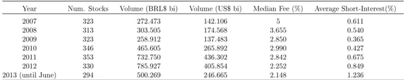
1.1 Summary Statistics: Brazilian Equity Loan Market Number of stocks is the number of different shares traded in stock loan market in a certain year. Volume is the financial volume, price times number of shares, of all stocks lent. Average fee is the mean of stocks daily loan fee, while daily loan fee is a value weighted average loan fee each day for each stock that accounts for the lenders fee and commissions fees. Short-interest is number of shares held in loan contracts normalized by the total number of shares outstanding, this measure is calculated daily for each stock and the average presented is the simple mean. . . 13
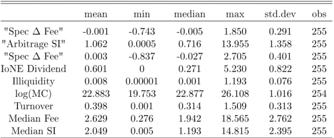
1.2 Summary Statistics for Arbitrage Contracts Return is defined as stock return minus IBRX50 return cumulated for 8 days beging at two days before the record date. Arbitrage loan contracts are the ones that generated tax benefits - i.e, borrowers are mutual funds and lenders are retail investors or foreign investors. Arbitrage Short-Interest is the total shares involved in arbitrage loan contracts divided by the total shares outstanding in the record day. 𝐴𝑟𝑏𝑖𝑡𝑟𝑎𝑔𝑒∆𝐹 𝑒𝑒 is the percentage increase of the loan fee in the event window for arbitrage contracts. The method for calculating 𝑆𝑝𝑒𝑐∆𝐹 𝑒𝑒 is analogous. IoNE is the IoNE dividend value as a percentage of the ex-date price. Turnover is the average daily turnover in the 21 business days before the IoNE dividend record date. The daily turnover is the traded volume in a day normalized by the market capitalization. Median loan fee is the median of average daily loan fee in the whole sample, whereas average daily loan fee is the value weighted average loan fee in a day. Median SI is the median short-interest for the whole sample. . . 13
1.3 Reduced Form Results Arbitrage Short-Interest is the total shares involved in arbitrage loan contracts divided by the total shares outstanding in the record day. 𝐴𝑟𝑏𝑖𝑡𝑟𝑎𝑔𝑒∆𝐹 𝑒𝑒is the percentage increase of the loan fee in the event window for arbitrage contracts. The method for calculating 𝑆𝑝𝑒𝑐∆𝐹 𝑒𝑒 is analogous. IoNE is the payout value as a percentage of the ex-date price. Liquidity is defined in Equation 1.3. Log MC is the log of Market Cap. Turnover is the average daily turnover in the 21 business days before the IoNE dividend record date. The daily turnover is the traded volume in a day normalized by the market capitalization. Median loan fee is the median of average daily loan fee in the whole sample, whereas average daily loan fee is the value weighted average loan fee in a day. Median SI is the median short-interest for the whole sample. Robust standard errors corrected for clustering at the ticker level.. . . 14
arbitrage contracts. IoNE is the payout value as a percentage of the ex-date price. Liquidity is defined in Equation 1.3. Log MC is the log of Market Cap. Turnover is the average daily turnover in the 21 business days before the IoNE dividend record date. The daily turnover is the traded volume in a day normalized by the market capitalization. Median loan fee is the median of average daily loan fee in the whole sample, whereas average daily loan fee is the value weighted average loan fee in a day. Median SI is the median short-interest for the whole sample. Robust standard errors clustered at the ticker level in parentheses. . . 15
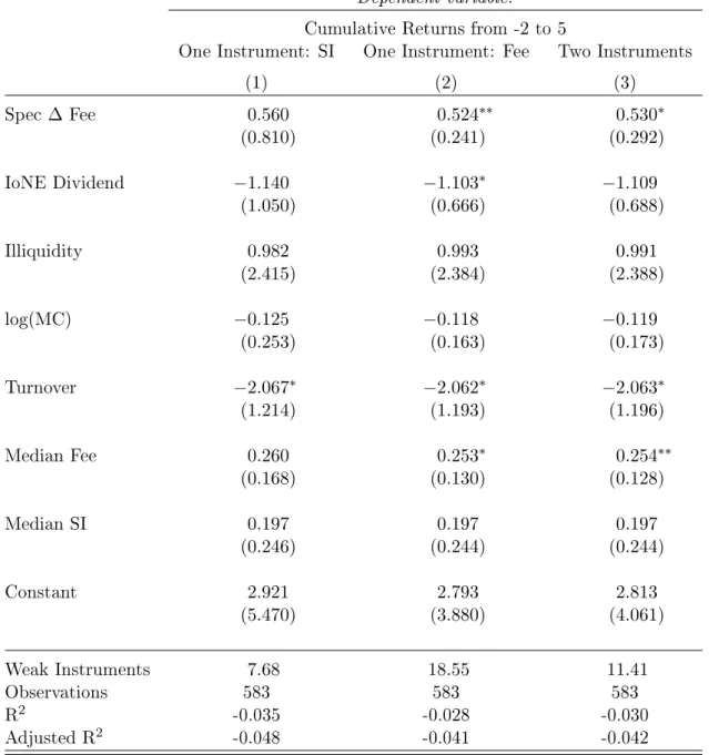
1.5 Unweighted Second Stage Regressions. This table shows the estimates of equation 1.4. The dependent variable is the cumulative returns.The method for calculating 𝑆𝑝𝑒𝑐∆𝐹 𝑒𝑒 is analogous. IoNE is the payout value as a percentage of the ex-date price. Liquidity is defined in Equation 1.3. Log MC is the log of Market Cap. Turnover is the average daily turnover in the 21 business days before the IoNE dividend record date. The daily turnover is the traded volume in a day normalized by the market capitalization. Median loan fee is the median of average daily loan fee in the whole sample, whereas average daily loan fee is the value weighted average loan fee in a day. Median SI is the median short-interest for the whole sample. Robust standard errors are clustered at the ticker level. . . 16
1.6 Instrument IoNE is the IoNE dividend value as a percentage of the ex-date price. Log MC is the log of Market Cap. Illiiquidity is defined in Equation 1.3. Turnover is the average daily turnover in the 21 business days before the IoNE dividend record date. The daily turnover is the traded volume in a day normalized by the market capitalization. Median SI is the median short-interest for the whole sample. Herfindahl Index (HI) is the sum of squares of each broker market share. Increases in the index indicate a decrease in competition. SI Before is the average short interest from 21 to 17 days before the event. Robust standard errors corrected for clustering at the ticker level.. . . 17
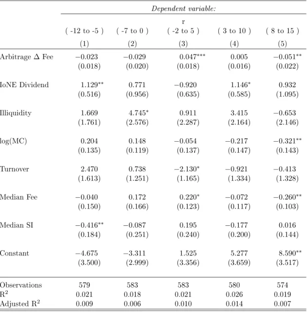
1.7 Reduced Form: Analyses of Persistence. The dependent variable is the cumulative in different periods.𝐴𝑟𝑏𝑖𝑡𝑟𝑎𝑔𝑒∆𝐹 𝑒𝑒 is the percentage increase of the loan fee in the event window for arbitrage contracts. IoNE is the payout value as a percentage of the ex-date price. Liquidity is defined in Equation 1.3. Log MC is the log of Market Cap. Turnover is the average daily turnover in the 21 business days before the IoNE dividend record date. The daily turnover is the traded volume in a day normalized by the market capitalization. Median loan fee is the median of average daily loan fee in the whole sample, whereas average daily loan fee is the value weighted average loan fee in a day. Median SI is the median short-interest for the whole sample.. Robust standard errors corrected for clustering at the ticker level. . . 18
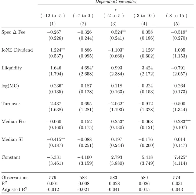
the delta fee in arbitrage transactions. Robust standard errors are clustered at the ticker level.The method for calculating 𝑆𝑝𝑒𝑐∆𝐹 𝑒𝑒 is analogous. IoNE is the payout value as a percentage of the ex-date price. Liquidity is defined in Equation 1.3. Log MC is the log of Market Cap. Turnover is the average daily turnover in the 21 business days before the IoNE dividend record date. The daily turnover is the traded volume in a day normalized by the market capitalization. Median loan fee is the median of average daily loan fee in the whole sample, whereas average daily loan fee is the value weighted average loan fee in a day. Median SI is the median short-interest for the whole sample. . . 19
1.9 Placebo test using normal dividends payout - Summary Statistics for "Arbitrage Contracts" Return is defined as stock return minus IBRX50 return cumulated for 5 days beging at two days before the record date. Arbitrage loan contracts are the ones that generated tax benefits - i.e, borrowers are mutual funds and lenders are retail investors or foreign investors. Arbitrage Short-Interest is the total shares involved in arbitrage loan contracts divided by the total shares outstanding in the record day. 𝐴𝑟𝑏𝑖𝑡𝑟𝑎𝑔𝑒∆𝐹 𝑒𝑒 is the percentage increase of the loan fee in the event window for arbitrage contracts. The method for calculating 𝑆𝑝𝑒𝑐∆𝐹 𝑒𝑒 is analogous. IoNE is the IoNE dividend value as a percentage of the ex-date price. Turnover is the average daily turnover in the 21 business days before the IoNE dividend record date. The daily turnover is the traded volume in a day normalized by the market capitalization. Median loan fee is the median of average daily loan fee in the whole sample, whereas average daily loan fee is the value weighted average loan fee in a day. Median SI is the median short-interest for the whole sample. . . 20
1.10 Placebo test using normal dividends payout - Reduced Form Results "Arbitrage Short-Interest"are loan contracts among arbitrage groups for the IoNE dividends divided by the total shares outstanding in the record day. 𝐴𝑟𝑏𝑖𝑡𝑟𝑎𝑔𝑒∆𝐹 𝑒𝑒 is the percentage increase of the loan fee in the event window for arbitrage con-tracts in the case of IoNE dividends. The method for calculating 𝑆𝑝𝑒𝑐∆𝐹 𝑒𝑒 is analogous. Normal Dividend is the payout value as a percentage of the ex-date price. Turnover is the average daily turnover in the 21 days before the IoNE dividend event. Average daily loan fee is the value weighted average loan fee in a day. Median loan fee is the median of average daily loan fee in the whole sample.Liquidity is defined in Equation 1.3. Robust standard errors corrected for clustering at the ticker level. Median SI is the median short-interest for the whole sample. . . 21
2.1 Summary Statistics This table reports summary statistics for the main vari-ables in our study. Short interest is the total borrowed shares over total shares outstanding. Each month, SD Fee is calculated as the monthly average of daily standard deviation of fees. Average Fee is the average value weighted loan fee. Short interest is the total of borrowed shares over total shares outstanding. Mar-ket Cap is represented in Millions. Book-to-marMar-ket ratio is calculated in the end of December of each year. The cases with negative book value are deleted. Herfin-dahl Index (HI) is the sum of squares of the market shares of the brokers. Increases in the index indicate a decrease in competition and an increase of market power . 38
shares outstanding. Herfindahl Index (HI) is the sum of squares of each broker market share. Increases in the index indicate a decrease in competition. Degree is simply the number of different brokers lending (borrowing) that stock in the last month. . . 39
2.3 Average Statistics per Year This table reports Number of Observations and the average values of our main variables for each year. N Obs is the number of observations,i.e. datapoints. N Stocks is the number of stocks composing the dataset that year. BM stands for Book to Market. Short interest is the total borrowed shares over total shares outstanding. Each month, SD Fee is calculated as the monthly average of daily standard deviation of fees. All values presented as year average . . . 40
2.4 Correlation Matrix This table shows the correlation between the variables used to sort the long short portfolios. SD Fee is the monthly average of daily standard deviation of fees; Avg Fee is the monthly average of daily average fees. Short interest is the total borrowed shares over total shares outstanding. DTC represents Days to Cover, i.e. the ratio between short interest and turnover. Each data-point here represent a monthly measure for a specific stock.. . . 40
2.5 Summary of Portfolio characteristics For each month we calculate the monthly (market cap weighted) average of each variable. This table displays the time series average for each variable. . . 40
2.6 Returns to Long Short Strategies Our main portfolio is based on loan fee dispersion, SdMLd, Small dispersion Minus Large dispersion. CMEw stands for Cheap Minus Expensive and relates to average loan fee. The remaining small minus large portfolios, SsiMLsi and SdtcMLdtc, are based on Short Interest and Days to Cover. Sharpe index based on annualized returns. . . 41
2.7 Market Factor Returns This table presents average returns, standard deviation of returns and sharpe ratio for the main market factors in Brazil. HML stands for High Minus Low ; SMB represents Small minus Big; Winners minus Losers is abbreviated as WML and finally IML relates to liquidity, Illiquid Minus Liquid. Those factors relate to Book to Market, Market Cap, Momentum and Liquidity, respectively . . . 41
2.8 Returns to portfolio strategies based on Loan Fee Dispersion This table provides portfolio alphas and loading, sorted on Loan Fee Dispersion. At the end of each month, all the stocks are sorted into three quantile: small (bottom 30%), Middle (40%), large (top 30%) deciles based on their loan fee dispersion at the end of each month. Portfolio returns are computed over the next month minus the monthly risk free rate - 30 day DI Swap. For the analysis we consider 5 factors: Market, Small Minus Big Factor (SMB), High Minus Low (HML), Winners Minus Losers (WML), Illiquid Minus Liquid (IML). The factors considered were extracted from NEFIN. Data runs from January 2007 to June 2013. ***, **, and * stands for significance level of 1%, 5% and 10%, respectively. . . 42
Middle (40%), large (top 30%) deciles based on their average loan fee at the end of each month. Portfolio returns are computed over the next month minus the monthly risk free rate - 30 day DI Swap. For the analysis we consider 5 factors: Market, Small Minus Big Factor (SMB), High Minus Low (HML), Winners Minus Losers (WML), Illiquid Minus Liquid (IML). The factors considered were extracted from NEFIN. Data runs from January 2007 to June 2013. ***, **, and * stands for significance level of 1%, 5% and 10%, respectively. . . 44
2.10 Returns to portfolio strategies based on Short Interest This table provides portfolio alphas and loading, sorted on Short Interest. At the end of each month, all the stocks are sorted into three quantile: small (bottom 30%), Middle (40%), large (top 30%) deciles based on their short interest at the end of each month. Portfolio returns are computed over the next month minus the monthly risk free rate - 30 day DI Swap. For the analysis we consider 5 factors: Market, Small Minus Big Factor (SMB), High Minus Low (HML), Winners Minus Losers (WML), Illiquid Minus Liquid (IML). The factors considered were extracted from NEFIN. Data runs from January 2007 to June 2013. ***, **, and * stands for significance level of 1%, 5% and 10%, respectively. . . 46
2.11 Returns to portfolio strategies based on Days to Cover This table provides portfolio alphas and loading, sorted on Days to Cover. At the end of each month, all the stocks are sorted into three quantile: small (bottom 30%), Middle (40%), large (top 30%) deciles based on their days to cover at the end of each month. Portfolio returns are computed over the next month minus the monthly risk free rate - 30 day DI Swap. For the analysis we consider 5 factors: Market, Small Minus Big Factor (SMB), High Minus Low (HML), Winners Minus Losers (WML), Illiquid Minus Liquid (IML). The factors considered were extracted from NEFIN. Data runs from January 2007 to June 2013. ***, **, and * stands for significance level of 1%, 5% and 10%, respectively. . . 48
2.12 : Fama-MacBeth Regressions This table reports results from Fama-Macbeth (1973) regression of monthly stock returns on Fee Dispersion, Average Fee, Short-Interest and Days to Cover. Fee Dispersion is the average daily standard deviation. Average Fee is the average value weighted loan fee. Short interest is the total of borrowed shares over total shares outstanding. Days-to-cover is short interest ratio over daily turnover. Size (log(MC)) is the natural log of firm market capitalization at the end of the June of each year. Book-to-market (log(BM)) is the natural log of book-to-market ratio calculated as end of December of each year. The cases with negative book value are deleted. The short term reversal measure (Reversal) is the lagged monthly return. All the t-statistics are Newey and West (1987) adjusted to control for heteroskedasticity and autocorrelation. ***, **, and * stands for significance level of 1%, 5% and 10%, respectively. . . 50
3.1 Average monthly excess returns for the test portfolios. The sample period is July 1963 to December 2014. Stocks are sorted into 3 portfolios based on the respective characteristic - book-to-market (BEME), operating profitability (OP) or investment (INV) and independently into 3 size (ME) groups. These are depicted row-wise and indicated in the first two columns. Last, portfolios are sorted into 3 further porfolios based on the loadings forecast, conditional on the first two sorts. These portfolios are displayed column-wise. The last column shows average returns of all 9 respective characteristic portfolios. The last row shows averages of all 9 respective loadings portfolios. In the top panels we use the low power and in the bottom panels we use the high power methodology. . . 74
depicted row-wise and indicated in the first two columns. Last, portfolios are sorted into 3 further porfolios based on the loadings forecast, conditional on the first two sorts. These portfolios are displayed column-wise. At each yearly formation date, the average respective characteristic (BEME, OP, or INV) for each portfolio is calculated, using value weighting. At each point, the characteristic is divided by the NYSE median at that point in time. The time series from 1963 to 2014 is then averaged to get the numbers that are presented in the table below. Note that, while sorts in the high power panels are based on industry-adjusted characteristics, the averages and medians are calculated based on the unadjusted characteristics. The last column shows average characteristics of all 9 respective characteristic portfolios. The last row shows averages of all 9 respective loadings portfolios. In the top panels we use the low power and in the bottom panels we use the high power methodology. . . 75
3.3 Sorting-factor exposures and five-factor alphas. The last column shows the return of long low-loading short high-loading hedge-portfolios. The last row shows averages of all 9 loadings portfolios. In the top panels we use the low power and in the bottom panels we use the high power methodology. Alphas and ex-post loadings on the relevant factor are obtained from a regression of monthly excess returns of the test-portfolios on the 5 Fama and French factors from July 1963 to December 2014. . . 76
3.0 Results of time-series regressions on characteristics-balanced hedge-portfolios. Stocks are first sorted based on size and one of book-to-market, profitability or investment into 3x3 portfolios. Conditional on those sorts, they are subsequently sorted into 3 portfolios based on the respective loading, i.e., on HML, RMW or CMA. For Mkt-RF and SMB we use the prior sort on size and book-to-market. The "hedge-portfolio"then goes long the low loading and short the high loading portfolios. On the bottom, we form combination-portfolios that put equal weight on three (HML, RMW, CMA), four (HML, RMW, CMA, Mkt-RF) or five (HML, RMW, CMA, Mkt-RF, SMB) hedge-portfolios portfolios. Monthly returns of these portfolios are then regressed on the 5 Fama and French factors in the sample period from July 1963 to December 2014. In Panel A we use the low power and in Panel B we use the high power methodology. . . 81
3.1 Results of time-series regressions on characteristics-balanced hedge-portfolios. Stocks are first sorted based on size and one of book-to-market, profitability or investment into 3x3 portfolios. Conditional on those sorts, they are subsequently sorted into 3 portfolios based on the respective loading, i.e., on HML, RMW or CMA. For Mkt-RF and SMB we use the prior sort on size and book-to-market. The "hedge-portfolio"then goes long the low loading and short the high loading portfolios. On the bottom, we form combination-portfolios that put equal weight on three (HML, RMW, CMA), four (HML, RMW, CMA, Mkt-RF) or five (HML, RMW, CMA, Mkt-RF, SMB) hedge-portfolios portfolios. Monthly returns of these portfolios are then regressed on the 5 Fama and French factors in the sample period from July 1963 to December 2014. In Panel A we use industry-adjusted characteristics and 36 monthly observations for beta forecasts. In Panel B we use un-adjusted characteristics, but separate es-timation of correlations and variances (with a 5 and 1 year window respectively) based on daily data and an additional intercept for the rank-year when estimating the loadings forecasts. . . . 82
1.1 Typical dates flowchart for the IoNE dividend event. . . 6
1.2 Distribution of Loan Fees By Firms by Year Figure shows the distribution of the average daily value-weighted loan fees in percentage points per year between January 2007 and June 2013. The vertical axis shows the frequency of firms with loan fees in the interval reported on the horizontal axis. . . 22
1.3 Payout Announcement . . . 22
1.4 Loan Fee around Record Date of an IoNE dividend event Figure shows the average loan fee around the record date of the IoNE dividend event. The daily loan fee for each share is the value weighed fee among all contracts in a certain day. The average loan fee is the common mean among shares. We consider 487 IoNE dividend events from January 2010 until June 2013. . . 23
1.5 Loan Fee around Record Date of an IoNE dividend event by Groups Arbitrage loan contracts are the ones that have tax benefits - i.e, borrowers are mutual funds and lenders are retail investors or foreign investors that took place before the record date and were liquidated after it. Speculative contracts are the other contracts. We define the daily loan fee as the value weighed average loan fee for each stock and each day around the IoNE date. The figure shows the average loan fee among all stocks for each day around the IoNE record date. . . 24
1.6 Short-Interest around Record Date of an IoNE Event Figure shows the average short-interest around the record date of the IoNE dividend event. The average short-interest is the common mean among shares. . . 25
1.7 Short Interest around Record Date of an IoNE dividend event by Groups Arbitrage loan contracts are the ones that have tax benefits - i.e, borrowers are mutual funds and lenders are retail investors or foreign investors that took place before the record date and were liquidated after it. Speculative contracts are the other contracts. We define the daily loan fee as the value weighed average loan fee for each stock and each day around the IoNE date. The figure shows average short interest among stocks for each day around the IoNE dividend record date. . 26
1.8 Abnormal Returns around the IoNE Dividend Date Figure show the cumu-lative abnormal returns starting from 10 days previous the record date. Abnormal return is calculated as the stock return minus the stock loading on the market port-folio IBX50, that accounts for the first 50 biggest stocks in market capitalization. The dotted line is the 95% percent confidence interval. . . 27
1.9 Reduced Form Coefficient for Different Return Windows Figure shows the estimated coefficient for different periods of 8-days cumulative returns. X-axis indicates the final date of 8-days cumulative returns, y-axis is the coefficient of 𝐴𝑟𝑏∆𝐹 𝑒𝑒 in reduced form regressions when considering as independent variables 𝐴𝑟𝑏∆𝐹 𝑒𝑒 and controls. The dotted line is the 95% percent confidence interval. . 27
𝑆𝑝𝑒𝑐∆𝐹 𝑒𝑒 in structural form regressions when considering just one instrument: 𝐴𝑟𝑏∆𝐹 𝑒𝑒and controls. The dotted line is the 95% percent confidence interval. . 28 1.11 Loan Fee around Record Date of an normal dividend event Figure shows
the average loan fee around the record date of the normal dividend event. The daily loan fee for each share is the value weighed fee among all contracts in a certain day. The average loan fee is the common mean among shares. We consider 487 IoNE dividend events from January 2010 until June 2013. . . 28
1.12 Short-Interest around Record Date of an IoNE Event Figure shows the average short-interest around the record date of the IoNE dividend event. The average short-interest is the common mean among shares. . . 29
1.13 Abnormal Returns around the Normal Dividend Date Figure show the cumulative abnormal returns starting from 10 days previous the record date. Ab-normal return is calculated as the stock return minus the stock loading on the market portfolio IBX50, that accounts for the first 50 biggest stocks in market capitalization. The dotted line is the 95% percent confidence interval. . . 29
2.1 Petrobras Loan Fee Histogram of fees paid by investors renting PETR4 (Petro-bras) on 30th April 2008 and April first 2009. The y-axis represents the number of contracts, x-axis shows the fee. . . 51
2.2 Mutual Funds Fee Relative Spread: Lender. Evolution of relative spread of loan fees received by individual person and foreign investors when compared to mutual funds . . . 52
2.3 Mutual Funds Fee Relative Spread: Borrower. Evolution of relative spread of loan fees paid by individual person and foreign investors when compared to mutual funds . . . 52
2.4 Loan fee Measures Over Time. Time series of aggregate measures. Each company daily average loan fee is calculated as the mean fee for contracts opened that day. The equal weighted cross sectional average composes our aggregated measure. The other aggregated measures are analogous. . . 53
2.5 Number of stocks for each portfolio. . . 53
2.6 Cumulative Returns for each long-short portfolio. . . 54
2.7 Transition Matrix The figure plots the transition probabilities of stocks across the three sd-fee sorted buckets over the period of one month. For example, the first column shows the percentage of stocks in the first bucket that end up in each of the three buckets after one month. . . 54
3.1 Rolling regression 𝑅2s – HML returns on industry returns This figure
plots the adjusted 𝑅2 from 126-day rolling regressions of daily HML returns on the
twelve daily industry excess returns. The time period is January 1981-December 2015. . . 68
3.2 HML loadings on industry factors. The upper panel of this figure plots the betas from rolling 126-day regressions of the daily returns to the HML-factor port-folio on the twelve daily industry excess returns over the January 1981-December 2015 time period. The lower panel plots only the betas for the Money and Bu-siness Equipment industry portfolios, and excludes the other 10 industry factors.
. . . 69
3.3 Volatility of the money and business equipment factors. This figure plots 126-day volatility of the daily returns to the Money and the Business Equipment factors over the January 1981-December 2015 time period.. . . 70
2015. . . 70
3.5 Ex-post loading vs. characteristic. This figure shows the time series average of post-formation factor-loading on the x-axis and the time series average of the respective characteristic on the y-axis of each of the 27 portfolios formed on size, characteristic and factor-loading. Panels A uses the low power methodology and B uses the high power methodology. The first row uses sorts on book-to-market and HML-loading, the second one operating profitability and RMW-loading and the last one investment and CMA-loading. . . 71
3.6 Portfolio Cumulative Returns. This figure plots the cumulative returns of of the five FF(2015) portfolios, and the residual portfolio. The residual portfolio is the equal-weighted combination of the HML, RMW, and CMA hedge portfolios, orthogonalized to the five-factors. Each portfolio assumes an investment of $1 at close on the last trading day of June 1963, and earns a return of (1 + 𝑟𝐿𝑆,𝑡+ 𝑟𝑓,𝑡)
in each month 𝑡, where 𝑟𝐿𝑆,𝑡 is the long-short portfolio return, and 𝑟𝑓,𝑡 is the one
1 Short-Selling Restrictions and Returns: a Natural Experiment 1
1.1 Introduction . . . 1
1.2 Stock Loan Market in Brazil . . . 4
1.3 The Tax Arbitrage . . . 5
1.4 Data . . . 6
1.5 Empirical Strategy: Identification and Specification . . . 7
1.5.1 Specification . . . 9 1.6 Results. . . 9 1.6.1 An Event Study . . . 9 1.6.2 Reduced Form . . . 9 1.6.3 First Stage . . . 10 1.6.4 Second Stage . . . 10
1.6.5 Determinants of Instrument Variation . . . 10
1.7 Falsification Tests . . . 11
1.7.1 Persistence Test and Reversal . . . 11
1.7.2 Placebo Test . . . 11
1.8 Conclusions . . . 12
1.9 Tables . . . 13
1.10 Figures. . . 22
2 Loan Fee Dispersion and the Cross-Section of Returns 30 2.1 Data, Variables and Summary Statistics . . . 33
2.2 Loan Fee Dispersion . . . 34
2.3 Loan Fee Dispersion and Returns . . . 36
2.3.1 Sorts on Loan Fee Dispersion . . . 36
2.3.2 Fama and MacBeth Regressions. . . 37
2.4 Conclusion. . . 37
2.5 Tables . . . 38
2.6 Figures. . . 51
3 The Cross-Section of Risk and Return 55 3.1 Introduction . . . 55
3.2 Theory . . . 58
3.2.1 Characteristic-Based Return Factors . . . 59
3.2.2 Relation between the characteristic-weighted and MVE portfolio . . . 59
3.2.3 An optimized characteristic-based portfolio . . . 61
3.3 Industry Factor Loadings . . . 61
3.4 Low- and High-Power Test Based Hedge Portfolios . . . 63
3.4.1 Construction of the factors and the set of test portfolios . . . 63
3.4.2 Postformation loadings . . . 65
3.6 Figures. . . 68
Short-Selling Restrictions and Returns:
a Natural Experiment
1
ABSTRACT
We estimate the causal impact of short-selling restrictions on returns. We take advantage of a unique dataset and exploit a source of exogenous variation in loan fees provided by a tax-arbitrage opportunity that existed in Brazil from 1995-2015. The tax-arbitrage opportunity stems from the fact that domestic mutual funds were exempted from income taxes on dividends received by stocks they borrowed, whereas the original owner would be taxed if she did not lend out the stock. Because we observe all equity loan transactions and transacting parts investor identity, we can distinguish equity lending motivated by tax-arbitrage from speculative transactions according to the borrower-lender match. We show that the loan fee on tax-motivated transactions is a source of exogenous variation to estimate the causal impact of the (endogenous) loan fee on stock prices. We find that increases in stock loan fees have strong impact on stock prices.
1.1 Introduction
Since the seminal article of Miller (1977), the impact of short-selling constraints on financial markets have been subject of numerous theoretical2 and empirical studies.3 A well known pre-dicted effect is that the interaction between heterogeneous valuations and short-sale constraint would lead to prices superior to the average valuation. Thus, both an increase in heterogeneity or in short-sale constraints would pressure prices upwards.4 While several empirical papers have convincingly illustrated the effect of the (cross-sectional and temporal) variation in heterogeneity
1This is a joint work with Marco Bonomo and João Manuel de Mello.
2e.g. Harrison and Kreps(1978), Diamond and Verrecchia (1987), Duffie, Garleanu, and Pedersen (2002), Scheinkman and Xiong(2003),Hong and Stein(2003),Hong, Scheinkman, and Xiong(2006),Blocher, Reed, and Wesep(2013)
3e.g. Chen, Hong, and Stein(2002a),Asquith, Pathak, and Ritter(2005a),Cohen, Diether, and Malloy(2007), Saffi and Sigurdsson(2011), Beber and Pagano(2013), Boehmer, Jones, and Zhang(2013), De-Losso, Genaro, and Giovannetti(2013),Kaplan, Moskowitz, and Sensoy(2013),Prado, Saffi, and Sturgess(2014)
and loan demand on stock prices,5documenting the effect of variation of stock loans supply poses a greater challenge.
Identification of the causal impact of short-selling restrictions on returns has been elusive for three reasons: data availability, lack of good measures of short-sale restriction, and, more importantly, the endogeneity of the decision to sell short. Several studies examined the effect of short-selling restrictions, but limited data availability has been always an issue (e.g., Cohen et al. (2007), Saffi and Sigurdsson(2011)). In most markets, lending services are provided over-the-counter by big custodian banks. Data are rarely available for any significant fraction of the market. For this reason, researchers have relied on proxies for short-sale constraints, such as institutional ownership for short supply and the Markit loan fee index for loan fee. However, these proxies tend to show little variation in the short-run.
The Brazilian security lending market provides a unique opportunity to circumvent the dif-ficulties with data. In contrast to other countries, all lending transactions are registered at a centralized platform - the BM&FBovespa. Because of the centralized nature of the market, we have access to a unique dataset containing all lending transactions, and their characteristics, such as type of borrower and lender (individual investors, mutual funds, etc.), contract length, borrowing fees, number of securities lent, among others.
Data availability is just one obstacle to the proper measure of the impact of short-selling restrictions on stock returns. Even more challenging is the fact that the decision to supply or demand equity loans is not random, and probably driven by investors’ (unobserved) expectations of future returns. One cannot infer causality by associating lending fees - as a measure of short selling constraints - with returns because fees are determined in equilibrium.
We explore an exogenous variation in the supply of loanable stocks provided by a tax arbitrage opportunity. Brazilian firms distribute two types of dividends: standard dividends and IoNE dividends (literally Interest on Net Equity or IoNE). For tax reasons, firms prefer IoNE dividends, which are treated as interest expenses. Shareholders pay a 15% tax rate on IoNE dividends, as opposed to an average of 25% that the firm pays on profits (equity holders are exempt from taxes on standard dividends).
Domestic mutual funds were exempt from the 15% tax on IoNE, and the tax status is deter-mined by the holder of the stock on the record date (not by the actual owner of the stock). Thus, transactions whose lender is not a domestic mutual fund and the borrower is a domestic mutual fund economize the 15% IoNe dividend tax. We show that the tax-arbitrage opportunity puts pressure on the lending market during IoNE dividend events, causing lending fees to rise sharply when the borrower, but not the lender, is a mutual fund. To a lesser but still very significant degree, fees also rise in transactions when the borrower is not a domestic mutual fund, which do not save the 15% IoNe dividend tax. We argue that the increase in lending activity from nondomestic mutual funds to domestic mutual funds which we call the taxarbitrage segment -is not related to the fundamental value of the firm. Thus, during IoNE events, the tax-arbitrage opportunity exogenously reduces the supply of loanable funds for short-selling purposes, which we call the speculative segment. In short, we have a quasi-natural experiment in the stock lending market.
We also deal with the incomplete price drop on the ex-dividend date, which challenges iden-tification strategies that explore dividend distribution events. In a nutshell, we exploit the fact that, while spot market transactions take three business days to settle, lending transactions are settled on the same business day. This allows us to isolate the incomplete price drop on the ex-dividend.
We have three findings. First, tightness in the tax-arbitrage segment causes abnormal returns in stock prices (the Reduced Form). More specifically, the larger the increase in lending fee in the tax-arbitrage segment, the higher the abnormal returns in stock prices during the days
5e.g. Chen et al. (2002a), Asquith et al. (2005a), Cohen et al.(2007), De-Losso et al.(2013), Prado et al.
surrounding the IoNE dividend event. During a typical event, stock prices have a 0.44% return in excess of the market accumulated over 8 trading sessions.
Second, tightness in the tax-arbitrage segments spills over to the speculative segment. The larger the increase of the lending fees in the tax-arbitrage segment, the larger the increase of lending fees in the speculative segment. This is the mechanism through which the exogenous shock propagates to share prices.
Finally, we use the increase in lending fees in the tax-arbitrage segment as a source of exoge-nous variation to estimate the causal effect of lending fees on stock prices (the Structural Form). During IoNE dividend distribution events, the average increase in the lending fees in the specula-tive market causes a 0.385% abnormal return in the stock price. Causal interpretation demands that increases in tightness in the tax-arbitrage segment have no direct impact on share prices (only through the lending fee for short-selling transactions). We provide evidence that this is a reasonable assumption in our setting.
The empirical literature has dealt with the problem of the endogeneity of short-selling restric-tions with varying degrees of success. Saffi and Sigurdsson (2011) explore a panel of stocks and associate lending supply and fees to several measures of price efficiency, such as bid-ask spreads. Their panel strategy with fixed-effects and a long time-series accounts for a large fraction of va-riation. However, it is not possible to guarantee that unobserved (to the econometrician) shocks are not driving simultaneously both returns (or bid-ask spreads) and fees or lending supply. In fact, earlier papers showed that short-interest predicted negative future abnormal returns, which suggests that short-interest has informational content (Cohen et al. (2007);Figlewski (1981).
Cohen et al. (2007) choose a different strategy. They postulate that higher fees associated with increases in lending indicate a (net) increase in the demand for shorting. Increases in fees coupled with reductions in lending represent a supply shock. They found that no significant effect of their identified supply shocks on returns. Their identification strategy implicitly assumes that supply shocks do not themselves contain any information about the returns, which in many settings can be a strong assumption. De-Losso et al.(2013), exploring a Brazilian sample as we do, define a supply shock as in Cohen et al. (2007), with the advantage of observing the size of the supply shock for each stock for a set of small stocks for which lending offers are public information. They found a significant negative relation between supply of loans and returns. Similarly toCohen et al.(2007), the identification strategy works only if the decision to change the supply is driven solely by factors other than opinions on the stock value.
According toPrado et al.(2014), stocks with higher concentration of institutional ownership tend to have lower lending supply. They found that higher concentration of institutional ow-nership is associated with higher idiosyncratic volatility of returns, limiting arbitrage. They show that demand shocks, as identified inCohen et al.(2007), generate substantially lower returns in stocks with higher concentration of institutional ownership. Chuprinin and Massa(2012) also use characteristics of institutional investors as proxies for short-sale constraints. When they instru-ment short-interest by those characteristics they obtain that higher short-interest is associated with higher return, corroborating the Miller hypothesis.
Boehmer et al.(2013) explores the short-sale ban of 2008 of more than 1,000 stocks, and find no price bump for these stocks. Their identification strategy is to match banned stocks with similar stocks that have never suffered the ban. Matching is an adequate procedure to account for observed heterogeneity, but the decision to ban short-selling of some particular stocks may be driven than factors unobserved to the econometrician (which may be the point of short-selling, namely, superior information).
Kaplan et al. (2013) perform a field experiment, randomly increasing the supply of stocks available for lending by a particular money manager. They find almost no impact on outcome variables such as returns and bid-ask spreads. Experimental data provides convincing exogenous variation. However, the supply shock may be too small to produce a quantitatively relevant impact.
From a methodological viewpoint, our work is closest to Thornock (2013) andBlocher et al.
(2013). Both analyze the effect of a restriction in the supply of shares around dividend events due to differential tax treatment between actual and replacement dividends.
Thornock (2013) finds that, around dividend events, the equity loan market gets tighter, with higher loan fees and lower short-interest. Similarly to our experiment, the differential tax treatment produces a negative shift supply of loanable shares. Thornock (2013) associates the negative shift in supply to market quality measures. One of them is the occurrence of average abnormal returns on ex-dividend dates. He finds that the dividend distribution events are associated with abnormal returns for high-dividend yield stocks and for stocks whose equity lending market was tight prior to the ex-dividend date.
Blocher et al.(2013) propose a framework for analyzing the impact of the equity loan market’s impact on share prices. In their model, short-selling restrictions have an impact on share prices only for hard-to-borrow stocks. FollowingThornock(2013), they use the increase in loan market tightness around dividend events as one of their strategies to test the model. They find that dividend distribution events are associated with abnormal returns around the ex-dividend date for stocks whose equity lending market is tight. Differently fromThornock(2013),Blocher et al.
(2013) measure tightness through lending rates, not short volume.
BothThornock (2013) and Blocher et al.(2013) measure the stock market return around ex-dividend dates. Hence, their results are subject to confounding effect of the incomplete price-drop phenomenon at ex-dividend date. In order to exclude this confounding effect, the ex-dividend data is the starting point of our cumulative return window. The only thing left is the increased tightness of the stock loan market around the record date.
Relative to the literature, we also move forward by documenting a clear mechanism behind the abnormal returns during dividend distribution events. Thornock (2013) andBlocher et al.
(2013) results are based on measuring abnormal returns during events when the equity lending market is arguably tight, a reduced-form object. Our data enables us to disentangle two equity lending markets: one affected (the tax arbitrage market) and one not affected by tax arbitrage opportunity (the speculative market). We have a clear mechanism: the tax-arbitrage opportunity, an exogenous shock, causes tightness in tax-arbitrage segment; tightness in the tax-arbitrage segment causes tightness in the speculative market, which, in turn, causes abnormal returns. Differently from received literature, we can directly link exogenous variation in lending fees to abnormal returns.
The paper is organized as follows. Section1.2gives an overview of the market for stock loans in Brazil. In Section1.3we explain the tax arbitrage opportunity that impacts the loan market in the period surrounding the IoNE payment dates. In Section 1.4 we describe the data used for the paper. In Section 1.5 we present our identification strategy. The results are analyzed in section 1.6. Section1.7 we present falsification tests. First we verify by changing the return window around the dividend record date, that the results we obtained cannot we reproduced for windows that are not consistent with the proposed mechanism. Then, we perform a placebo test by reproducing our empirical strategy around ordinary dividend dates. The last Section concludes.
1.2 Stock Loan Market in Brazil
Similarly to other countries, trading in equity loan market in Brazil is mostly over-the-counter (OTC). Differently from other countries, all loan contracts must be registered in the Brazilian stock exchange, BM&FBovespa. BM&FBovespa acts as a clearing platform, and as a central counterpart. It guarantees all loan contracts, and keeps track of the contract collateral.
A typical lending operation involves the exchange and four different participants: the lender, the borrower, the lender’s broker and the borrower’s broker. The cost to borrow a stock is the loan fee (which includes both brokers commission fees), plus an exchange fee of 0.25% annually.
Table 1.1 contains summary statistics about the Brazilian equity loan market from 2007 through 2013. In this period, the number of stocks lent became approximately constant at 300. However, other statistics indicated that the stock loan market gained importance. The average annual growth in the volume of equity lending was 23.5%. The average short-interest doubled, reaching 1.236% in 2013. Average loan fees dropped by an average 43 basis points (bps) per year, from 5% to 2.148% rate. On the lending side, retail investors, domestic mutual funds and foreign investors represent approximately 90% of the market. Borrowers are mostly domestic mutual funds (56.7%) and foreign investors (27.8%)
Figure1.2depicts the distribution of the average loan fees for each stock from January 2007 through June 2013. Fees are high in Brazil, relative to more mature markets. 20% of the fees charged were higher than 6% per year. Nevertheless, the performance of the lending market is improving rapidly, according to this metric, with the whole distribution shifting to the left (Figure1.2).
1.3 The Tax Arbitrage
Until a change in law in August 2014, a loophole in the tax law provided a tax-arbitrage oppor-tunity involving equity lending.
Brazilian firms distribute profits through two types of dividend, standard and IoNE dividends (literally Interest on Net Equity). The difference is the tax treatment. The IoNE dividend was created in 1995 with the stated goal of incentivizing firms’ capitalization. Corporate taxable income is reduced by the distribution of IoNE dividends, but shareholders pay a 15% tax rate (the same rate as interest on long-term debt, thus the name Interest on Net Equity). Standard dividends are not deducted from the corporate taxable income, but their recipients are exempt from taxation. In Brazil the law requires the distribution of a minimum of 25% of profits.6 Firms prefer to distribute IoNE dividends because the corporate tax rate is 25%, and thus IoNE dividends economize on taxes. In fact, there is an upper limit to the amount of IoNE dividends distributed, but not to standard dividends. Firms can distribute IoNE dividends up to the smallest of three following numbers: the net worth times the Long-Term Interest Rate (a prime rate determined by the federal government), 50% of the current period earnings before corporate taxes, and 50% of the accumulated earnings and reserves in previous periods.
In order to avoid double taxation, mutual fund and investment clubs are exempt from security earning taxes, since funds shareholders pay taxes on the NAVs appreciation. The difference in tax treatment between types of investors generated a tax arbitrage until the August 2014 law closed the loophole. Since the borrower was considered the owner of the stock for tax purposes, funds could borrow a stock from a taxable investor during the period of its IoNE dividend distribution and receive the full dividend amount. They had to pay the original stockholder only the dividend net of the 15% of taxes, retaining the difference. Taxable stock lenders (e.g. retail and foreign investors) and brokers could appropriate part of the funds gains by increasing their lending and brokerage fees, respectively.
Relevant dates for dividend distribution in Brazil are similar to those in the United States. Figure1.1 depicts the flowchart of important dates for our empirical exercise in a typical IoNE distribution affect. The first date is the earnings’ announcement day, an official public statement of a company’s information for a specific period, typically a quarter. On earnings’ announcement date, investors get to know the company’s distribution policy, including the amount of payouts in the form of standard and IoNE dividends. Earnings’ announcements usually cluster around the
6Almost all companies in our sample operate under the so-called Real Income regime. The Real Income
regime is progressive. Companies pay a 15% tax rate on annual incomes up to BRL 240,000.00, approximately USS89,000.00; above this threshold companies pay an additional 15% surcharge. Almost all companies in our sample have annual income well above the threshold. The tax rate is then about 24% for those companies. In contrast, the tax rate on IoNE dividends is 15%. Thus, when corporations choose to distribute, they almost always distribute through IoNE up to the legal. Firms often choose to distribute the minimum of 25% of profits.
earnings’ season. The second date is the payout announcement day (also called the declaration day), when the next IoNE dividend payment is announced, as well as the ex-dividend, record, and payment dates. The payout announcement usually happens a month after the earnings’ announcement. The next is the date day. Stocks bought in the spot market on or after the ex-date do not receive the announced IoNE. The ex-ex-date is at least one business day after thepayout announcement. The record date day determines eligibility to the IoNE dividend. Holders of the stock as shown in the company’s books at the record date are entitled to the IoNE dividend. Because it takes three trading days for a stock transaction in the spot market to be settled, the ex-date is two trading days before the record date day and the last cum day is three business days before the record date day. Since stock loan transactions are registered immediately, when some investor borrows a stock before the register day, she is entitled to receive its dividend payment. Therefore, the borrower has two days more than the buyer to do the transaction in time to have the right to receive the dividend. We will exploit this lag for identification purposes. Finally, the payment date is when the IoNE dividend payment is made. The payment date varies considerably.
Figura 1.1: Typical dates flowchart for the IoNE dividend event.
1.4 Data
BM&FBovespa keeps detailed records of all lending transaction. We observe the whole process: offers, contracts, and liquidation. We also observe information about investors, brokers, and maturity.
The data set runs from January 2010 to June 2013. We use the following data: contract date, liquidation date, loan fee, quantity of shares and investor type. We merge the BM&FBovespa data with the Radar dataset, which contains information about payout events. Merging the two datasets allows us to identify loan transactions that are eligible for tax arbitrage, the tax-arbitrage contracts, and non-eligible transactions, the speculative contracts.
We define a loan contract to be tax-arbitrage driven if and only if it has three characteristics: 1) the lender is a taxable investor and borrower can receive IoNE dividends exempt from taxes (mutual funds and investment clubs); 2) it takes place the day or before the record date; 3) it is liquidated after the record date. All other contracts are considered speculative driven.
Information on stocks returns and traded volume are from Economática. We use abnormal returns, the stock return minus the market portfolio, measured by the IBX50 7. For each IoNE dividend event, we specify a window which includes 21 days before and after the event. Returns are defined as:
𝑟𝑡,𝑡+1= 𝑙𝑜𝑔
(︂ 𝑃𝑡+1+ 𝑁 𝐷𝑡+1 𝑃𝑡
)︂
where 𝑁𝐷 stands for net dividends, i.e., gross dividends discounted with the highest tax rate. We isolate the imperfect ex-dividend date price drop effect by considering returns after the ex-dividend date. In short, dividend adjustment in returns is not a concern.
The loan fee of a given stock in a given day is the value-weighted average fee of loan contracts that took place that day. ∆𝐹 𝑒𝑒 is the percent change in the loan fee inside and outside of the event. Inside the event means within 5 trading days of the record date. Outside means belonging to the interval [−21, −17] ∪ [17, 21], where 0 is the IoNE record date8.
∆𝐹 𝑒𝑒 = 𝐹 𝑒𝑒𝑖𝑛− 𝐹 𝑒𝑒𝑜𝑢𝑡
𝐹 𝑒𝑒𝑜𝑢𝑡 (1.1)
We also calculate an illiquidity measure following Amihud (2002). We measure stock 𝑖 illi-quidity at day 𝑡 as the average ratio of the daily absolute log return to the trading volume on that day, as described in equation 1.2. For every event, we calculate the average illiquidity for that stock in the last 252 business days, as described in equation1.3.
𝐼𝑙𝑙𝑖𝑞𝑢𝑖𝑑𝑖𝑡𝑦𝑖𝑡= |𝑙𝑛(𝑟𝑖𝑡)| 𝑉 𝑜𝑙𝑢𝑚𝑒𝑖𝑡 (1.2) 𝐼𝑙𝑙𝑖𝑞𝑢𝑖𝑑𝑖𝑡𝑦𝑒𝑣𝑒𝑛𝑡= 1 𝑁𝑒𝑣𝑒𝑛𝑡 𝑁𝑒𝑣𝑒𝑛𝑡 ∑︁ 𝑡=1 |𝑙𝑛(𝑟𝑖𝑡)| 𝑉 𝑜𝑙𝑢𝑚𝑒𝑖𝑡 (1.3)
The IoNE dividend event has to satisfy certain criteria to be in the sample. There must be arbitrage contracts starting in the five days before the record date of the event. Stocks must have had been traded during all 21 trading days before and after the record date. We demand that we have data on turnover during all 21 trading days before the record date. We trim outliers by discarding the 1% highest returns in the sample9. Events in sample include stocks that represent 70% of BM&FBovespa market capitalization. Table 1.2 contains summary statistics for those events.
Summary statistics hint at our main results. Stocks show an average 0.48% return over the IBRX50 index in a 8-trading-day period around the IoNE dividend event, but dispersion is large. Total short-interest increases drastically. Fees on arbitrage contracts increase fivefold, reflecting the fact that lenders appropriate part of the tax arbitrage profit. Fees on speculative contracts also increase significantly, 73%. The amount of IoNE dividend distributed is roughly 0.23% of the companies’ market cap.
1.5 Empirical Strategy: Identification and Specification
The IoNE dividend distribution events provide exogenous variation to estimate the causal impact of short-selling restrictions on returns. We deal with two elusive problems: the endogeneity of the changes in lending fees, and the contamination of the incomplete ex-dividend price drop.
The tax arbitrage opportunity described in1.3provides quasi-natural experimental variation in lending fees on speculative lending transaction (i.e., borrowing to short sell).
During events of IoNE dividend distribution, the lending market split into two segments. In the tax-arbitrage segment, lenders that are subject to tax withholding (retail and foreign investors, banks, and firms) lend to borrower that are tax exempt (domestic mutual funds). The speculative segment contains all transactions conducted between all other combinations of lender-borrower pairs (e.g., domestic mutual funds lending to domestic mutual funds). Because
8For robustness, we tried different intervals for the Δ𝐹 𝑒𝑒 calculation, as well as using the maximum fee in
each period instead of the mean. The results are unchanged and are available upon request.
9For robustness, we also trimmed at the following cutoffs: 0%, 5%. Results are similar and are available upon
they do not generate any tax benefit, we assume that stock borrowing in this segment is done for speculative reasons.
Because of the tax arbitrage opportunity, the events of IoNE dividend distribution severely disrupted prices and quantities in the lending market.
Figure1.4depicts fees on 242 trading days around the IoNE dividend event. Between 21 and 9 days before the event, fees average 2.6%. After that, fees increase, reaching an impressive 10.4% at the record date. Quite interestingly, most the increase in fees occurs during the three-day period that precedes the record date.
Figure 1.5 splits the dynamics of loan fees for tax-arbitrage and speculative loan contracts. The increase in average loan fees in figure1.4stems mostly from tax-arbitrage contracts.
The pressure in the tax-arbitrage segment spills over to the speculative segment. Albeit less dramatically, fees on speculative contracts increase significantly, from 2.66% to 3.68%, a 38% increase.
Figure1.6depicts the short-interest around the event. Twenty-one days business days before the record date the average short-interest on tax-arbitrage contract was, on average, 1.51% of volume. They increase to 3.44% on the record date. In contrast, short-interest on speculative drops, from 1.47% to 0.96% of volume on average, a 35% drop.
Average changes in short interest and fees suggest that, during IoNE dividend events, the demand for borrowing stocks increases in the tax-arbitrage segment, and the supply of loanable stocks to speculative segment contracts.
We go beyond averages. We explore the heterogeneity across IoNE distribution events in the magnitude of the increase in the fees of the tax-arbitrage transactions. We show the following chain of causation. During events in which the fees and short-interest in tax-arbitrage segment increase more steeply, fees in the speculative segment also increase more. Moreover, the more fees increase in the speculative segment increase, the larger the increase in stock prices.
In summary, we estimate the causal effect of short selling constraints on returns by using the increases in lending fees in the arbitrage segment as a source of exogenous variation for the fees of the speculative segment.
The identification hypothesis is that, during IoNE distribution events, contracts in arbitrage segment do not reflect investors expectations about future returns. This is a reasonable as-sumption because in this period lending fees in the tax-arbitrage segment are just too high to rationalize short selling stocks (if borrowers short sell the borrowed stock they are not entitled to the dividend payment). Around IoNE dividend events, one can safely assume that stocks borrowed for tax-arbitrage purposes are not sold in the spot market. Therefore, it reasonable to assume that the changes in fees in the tax-arbitrage segment are exogenous to return expectations in the spot market.
We also deal with the incomplete ex-dividend price drop, a threat to identification in studies that use dividend distribution events that pressure lending markets (Frank and Jagannathan
(1998),Elton, Gruber, and Blake(2005)). The incomplete ex-dividend drop produces abnormal positive returns in spot market in periods around dividend distribution events. Differently from the previous literature, we explore the fact that spot and lending transactions are settled on different dates. Spot market operations take three business days to be settled, which implies that the ex-dividend date is two days before the dividend record date. In contrast, lending operations are settled on the same business day, and most of the arbitrage driven loans actually take place on the record date and not on the ex-date. We avoid capturing the incomplete price drop at ex-dividend date by restricting the analysis to cumulative returns accruing from the ex-dividend date onward. The assumption is that any information or abnormal return due to the dividend distribution is already factored into prices by the ex-date.
1.5.1 Specification
The main object of interest is the impact of speculative (non-arbitrage) fees on returns, which provides a measure of the impact of short-selling restrictions on returns. Our main regression of interest is:
𝑅𝑒𝑡𝑢𝑟𝑛𝑒𝑖= 𝛼 + 𝛽𝑆𝑝𝑒𝑐∆𝐹 𝑒𝑒𝑒𝑖+ 𝐶𝑜𝑛𝑡𝑟𝑜𝑙𝑠𝑒𝑖+ 𝜀𝑒𝑖 (1.4)
The subscript 𝑒 stands for IoNE event, defined as the 8-days period from the ex-dividend date. Subscript 𝑖 stands for stocks. 𝑅𝑒𝑡𝑢𝑟𝑛𝑒𝑖is the cumulative return in the event window 𝑒 and stock 𝑖, 𝑆𝑝𝑒𝑐∆𝐹 𝑒𝑒 is the change in the fee on speculative contracts during the event. Controls include IoNE dividend as a percentage of the ex-price, illiquidity, market cap, turnover, median fee and median short interest. Notice that a lower expected return on the stock should lead to an increase in short-selling activity and an increase in the lending fee in the speculative market. This makes 𝑆𝑝𝑒𝑐∆𝐹 𝑒𝑒 endogenous, biasing the OLS estimation results.
In order to overcome the endogeneity problem we use two instruments: increases in fees and short-interest on arbitrage transactions. The hypothesis is that changes in the fees and short-interest on arbitrage transactions contain no relevant information for returns in the event window.
The first stage is:
𝑆𝑝𝑒𝑐∆𝐹 𝑒𝑒𝑒𝑖 = 𝛽0+ 𝛽1𝐴𝑟𝑏𝑆ℎ𝑜𝑟𝑡𝐼𝑛𝑡𝑒𝑖+ 𝛽2𝐴𝑟𝑏∆𝐹 𝑒𝑒𝑒𝑖+ 𝐶𝑜𝑛𝑡𝑟𝑜𝑙𝑠𝑒𝑖+ 𝜖𝑒𝑖
(1.5) We take a conservative stance and cluster observations at the ticker level when estimating standard deviations.
1.6 Results
1.6.1 An Event Study
The Miller hypothesis implies that events in the lending market spillover into the spot market. Before presenting our main results, we perform an event study for IoNE dividend distribution to calculate the average excess return around the IoNE dividend record date. Figure1.8depicts the cumulative excess return starting 10 days before the record date. The 10-day cumulative return on the record date is 83bps (significantly positive at 5% confidence level). Inspection the dates around the record date, shows that the positive excess return persists for some days after record date.
1.6.2 Reduced Form
Table 1.3has the results of the reduced-form. In column (1) we include only changes in short-interest among tax-arbitrage transactions (besides the controls). The estimated coefficient, 0.062, means that the mean tax-arbitrage short-interest - 2.458 percentage point. - is associated with a non-significant abnormal returns of 2.458 × 0.062 = 0.15 percentage points cumulated over eight trading sessions. In column (2) we regress the abnormal returns on the size of the increase in fees in tax-arbitrage transactions. We find that the mean increase on fee of arbitrage contracts causes a 0.23% abnormal return. When both instruments are included, only Arbitrage ∆ fee matters (column (3)). We find no impact on abnormal returns of increases in fees in specula-tive transactions (column (4)). This is not surprising because most of the variation in fees in speculative transactions is endogenous. Finally, in column 5 we include the instruments and the endogenous variable, and reach the same conclusions as in columns 1 through 4. In summary, changes in loan fee in the tax-arbitrage transactions are associated with abnormal returns, which
is compatible with the idea that the tax-arbitrage tightness in lending markets increase share prices.
1.6.3 First Stage
Table 1.4 presents the first stage results. Column (1) presents the results of the regression of variation of speculative fees on one instrument, the short-interest of tax-arbitrage transactions. Short-interest in tax-arbitrage transactions cause increases in fees on speculative transactions. The relationship is not strong enough when considering just this instrument (partial F -statistic of 7.68) and weak instruments issues may be a concern. Column (2) is the same regression but the instrument is the change in tax-arbitrage transactions. The estimated coefficient means that a typical increase tax-arbitrage loan-fee - 5.080 - causes a (5.080 × 0.089) * 100 = 45.2 percentage point increase in fees in speculative transactions, a large increase (fees are normally 1 percentage point). In this case, the partial F -statistic is 18.55 and weak instrument is not a concern. In Column (3) we include both instruments.
1.6.4 Second Stage
Table 1.5 presents results for the second stage. The columns are equivalent to the models presented in the last section. We concentrate on the second column, for which the instrument is the Arbitrage ∆ Fee. The estimated coefficient on changes in speculative fees is 0.524, and quite precisely estimated (p-value less than 1%). The estimated coefficient means that the typical increase in speculative fees - 73.5% - causes a 0.385 percentage point abnormal return in share price. The exogenous increase in speculative fees is large enough to make short-selling less attractive, producing a large increase in share prices, at least in short-run.
1.6.5 Determinants of Instrument Variation
In order to investigate if the assumptions about our chosen instrument are empirically plausible, we regress the variation in loan fee for the arbitrage contracts on several variables. Our hypothesis is that the tightness in arbitrage market is mainly driven by the amount of income that could be engendered by fiscal arbitrage operations. Since, the amount of taxes on IoNE dividend distribution is the upper bound on the income generated by evaded taxes in those operations (and the tax rate is constant), the IoNE dividend distribution per share, and the market capitalization seem plausible determinants of the tightness of this lending market. Notice, that the IoNE dividend per share distribution is announced at earnings date, which is many days earlier than our event window. Thus, it should not contain any information about stock market return in our event window. Table1.6corroborates our hypothesis, since both market capitalization and IoNE dividend per share are positively and significantly related to the loan fee for arbitrage contracts. This result holds, in regressions when each of those variables is the only explanatory variable, when both are combined, or when both are combined with other regressors.
We also test for some characteristics microstructure of the lending market that could affect the impact of the induced arbitrage operations on the lending fee, and for controls considered in the main regressions. We test for illiquidity, turnover, median short-interest over the whole sample, the short interest before the event window, the Herfindal index among lenders’ and borrowers’ brokers. However, none of those variables seems to be related with our instrument. In summary, one can assume that, conditional on the variables related to the magnitude of the IoNE dividend distribution, the variation left in tightness of the tax-arbitrage market is as good as random.
1.7 Falsification Tests
For robustness, we perform two exercises. First, we analyze the returns in different windows around the IoNE dividend record date. Second, we use normal dividends payout as a placebo test for our main exercise.
1.7.1 Persistence Test and Reversal
Figure 1.9 shows the estimated reduced-form parameters over different windows of analysis, always accumulating 8-trading days. We see a clear pattern. The impact of loan fee in the tax-arbitrage transactions on abnormal return happens exactly when we should expect, reaching a peak in the window that includes the record date. For other periods, the impact is hardly distinguishable from zero. As shown in Table 1.7, it is very interesting that when considering cumulative returns from 8 to 15 after the recode date, the estimated coefficient of -0.519 (signifi-cant at 10% level), indicating a reversal of almost the same magnitude as the positive abnormal returns around the record date.
Figure 1.10 shows the estimated structural parameters over different windows of analysis, always accumulating 8-trading days. Again, the pattern is clear. The structural parameter, the causal effect of speculative transactions’ changes in fees on abnormal return happens exactly when we should expect, reaching a peak two days after the record date. For other periods, the impact is not distinguishable from zero, but in the end of the period. Precise coefficients are shown in Table1.8.
1.7.2 Placebo Test
One may suspect that our empirical findings are a feature of the dividend events, being unrelated to the tax arbitrage mechanism we proposed. In order to disentangle this alternative hypothesis from the tax arbitrage effect, we repeat the same tests around ordinary dividend dates. Since ordinary dividends are not taxable in Brazil, there are no tax arbitrage operations involving stock loans around ordinary dividend dates. Therefore, normal dividend events are ideal to construct a placebo test for the effect of tax arbitrage.
We repeat the same methodology described in Section 1.5, now considering just normal dividends events. We do not consider normal dividends events for which the record date is less than 21 days of IoNE dividend date, since those events would be contaminated by the short-restriction caused by the arbitrage opportunity. All others filters are exactly the same as it was done for IoNE events.
In figure 1.11and 1.12we can see that around the record date of the normal dividend there is no particular spike either on the loan fee neither on the short interest.
We present the summary statistics for the normal dividends events in Table1.9. The results of the reduced form regressions are shown in Table 1.10. It is interesting to notice that in this case Arbitrage Short Interest and Arbitrage ∆ Fee are endogenous variables, since they should reflect the willingness to short of investors. Contrary to our main results, here we found that they have negative impact on returns, which is the result normally found in the literature. The interpretation is that the trading activity of informed short sellers is more intense when they have negative information about the stock performance. Recall that in our initial experiment, a higher arbitrage fee (or short interest) indicated an exogenous constraint to short selling. The increased demand for short selling due to tax arbitrage left less room for investors willing to short sell due to speculative reasons. The difference in outcomes between the IoNE and common dividend exercises should reflect the importance of tax arbitrage in generating our main results.
1.8 Conclusions
Despite an intense debate about the impact of short-selling restriction price, the evidence regar-ding the effects of short sales on asset prices is mixed. The lack of consensus is in large part due to two difficulties. First, identifying a clear source of exogenous variation in supply and demand for stock loan. Second, lack of data availability on lending due to the OTC nature of these markets in most countries. Our study estimates the causal impact of short-selling restrictions on returns by taking advantage of a unique dataset and a unique source of exogenous variation in rental fees. One standard-deviation increase in loan fees causes a 1.11% of returns above the market over 8 trading days. This is strong evidence in favor of Miller’s Hypothesis.