Efficient frontier and capital market line on PSI 20

M

ASTER OF

S

CIENCE IN

F

INANCE

M

ASTERS

F

INAL

W

ORK

D

ISSERTATION

E

F

A

C

M

L

20

BY

:

D

A

B

M

ASTER OF

S

CIENCE IN

F

INANCE

M

ASTERS

F

INAL

W

ORK

D

ISSERTATION

E

F

A

C

M

L

20

B

:

D

A

B

S

:

P

.

M

T

M

G

I

Abstract

This work estimates the efficient frontier of Markowitz and the capital market line for the Portuguese stock market, considering two different periods, before and after the 2008 financial crisis. The results show the strong impact on the global minimum variance portfolio and the market portfolio, with surprising conclusions. The sensitivity of the results to the period’s length is also considered and remarkable.

K

:

II

Acknowledgment

I would like to express my special thanks to my supervisor, Prof. Maria Teresa Medeiros Garcia, for her commitment, availability and support through the elaboration of this dissertation and to Prof. Clara Raposo, for all the help and concern through the master course.

And last, but not least, for my girlfriend, for the patient and for being the first one to always believing in me, and for my family and friends for all the encouragement, learnings and discussions that help me improve and achieve my goals. I’m grateful to everyone who made this possible.

III

Contents

1. Introduction………1

2. Theoretical Framework and Literature Revision………...3

2.1. Basic Concepts…...………..3

2.1.1. Return………..3

2.1.2. Risk………..4

2.1.3. Covariance and Correlation……….4

2.2. Modern Portfolio Theory ……….5

2.2.1. Mean-Variance Theory………...8

2.3. Efficient Frontier………..11

2.4. Capital Market Line and Separation Theorem………...13

2.5. Investor Profile………....16

2.6. Performance Measures………...18

2.6.1. Sharpe’s Ratio………...………..19

2.7. Optimal Portfolio Selection………...20

3. Analysis of the Portuguese Stock Index………..………..22

4. Data Set and Methodology………..………25

5. Results………..………..31

6. Conclusion……….……….36

7. References……….………38

IV

Figures List

Figure 1 – Efficient Frontier………...12

Figure 2 – Capital Market Line ……….15

Figure 3 – Risk Utility Function ………18

Figure 4 – Optimal Portfolio Selection ………21

Figure 5 – Data Summary (Post 2009 Period)……….………...V Figure 6 – Data Summary (Pre 2009 Period)………...V Figure 7 – Variance-Covariance Matrix (Post 2009 Period)………...VI Figure 8 – Variance-Covariance Matrix (Pre 2009 Period)………...VI Figure 9 – Portfolio Performance (Post 2009 Period)………...VII Figure 10 – Portfolio Performance (Pre 2009 Period)………...VIII Figure 11 – Data Resume (Pre 2008 Period)……….IX Figure 12 – Portfolio Performance (Pre 2008 Period)………X

V

Graphics List

Graph 1 – Evolution of PSI20………...25

Graph 2 – Return vs. Risk (Post 2009 Period)………...28

Graph 3 – Return vs. Risk (Pre 2009 Period)………....28

Graph 4 – Efficient Frontier (Pre and Post 2009 Periods)………31

Graph 5 – Capital Market Line (Pre and Post 2009 Periods) ……….33

Graph 6 – EF and CML (Pre and Post 2009 Periods)………..34

Graph 7 – EF and CML (Pre 2008 and Pre 2009 Periods) ……….35 Graph 8 – EF and CML (Post 2009 Period)………...VII Graph 9 – EF and CML (Pre 2009 Period)………VIII Graph 10 – EF and CML (Pre 2008 Period)……….…...IX

1

1 Introduction

This dissertation has as the final objective the determination of the efficient frontier of Markowitz (EF) and the capital market line (CML), for the Portuguese case, considering two different periods. These different periods will make us understand what happen to the design of the EF and CML in the pre and post financial crises.

Under the assumption of the economic rationality, investors choose to keep efficient portfolios, i.e., portfolios that maximize the return for a certain level of risk or that minimize the risk for a certain level of expected return, always considering investors demands. According to Markowitz (1952, 1959), these efficient portfolios are on the opportunity set of investments, that we can refer to as the par of all portfolios that can be constructed from a given set of assets.

While the classic portfolio theory says that the assets selection is determined by the maximization of the actual value of the expected value, the modern theory defends that the investment strategy must be conducted in a risk diversification perspective, what leads to an analysis on the combination of assets considering the return and the risk, and also the covariance of the returns between the assets. Mean-variance theory is a solution to the portfolio selection problem, assuming that investors make rational decisions.

Considering Markowitz modern theory, the optimal portfolio should be the tangency portfolio between the EF and the indifference curve or, in other words, the EF with greater utility. Under the economic theory of choice, an investor

2

chooses among the opportunities by specifying the indifference curves or utility function. These curves are constructed so that along the same curve, the investor is equally happy, what leads to an analysis on the assumed investor’s profile.

Tobin (1958) introduced leverage to portfolio theory by adding a risk-free rate asset. By combining this risk-free asset with a portfolio on EF, we can construct portfolios with better outcomes that the ones simply on EF. This is represented by the CML, which is a tangent line from the risk-free asset till the risky assets region.

The tangency point originated by the combination of the CML and the EF represent the searched optimal portfolio.

Our work follows the following structure: in the second section, we present the theoretical framework and literature review, under the theories developed by the authors regarding the EF, CML and the choice of the optimal portfolio. In the third section, we make an analysis on the PSI20 and the comparison between some model assumptions and the real functioning on the Portuguese stock market. Data set and methodology used for the work is discussed in the fourth chapter, with the results presented in section five. Finally, the conclusion is presented in section six.

3

2 Theoretical Framework and Literature Review

In this section we review some basic concepts of modern portfolio theory, the efficient frontier and the capital market line. The investor profile and performance measures are presented to determine the optimal portfolio.

2.1 Basic Concepts

2.1.1 Return

The return of a financial security is the rate computed based on what an investment generates during a certain period of time, where we include the capital gains/losses and the cash-flows it may generate (dividends, in the case of stocks). We can calculate the returns by the difference between an asset price at the end and in the beginning of a selected period, divided by the price of the asset at the beginning of the selected period.

𝑅_𝑡 = 𝑃𝑡− 𝑃𝑡−1

𝑃𝑡

Where:

𝑅_𝑡 is the return on moment t;

𝑃_𝑡 is the asset price on moment t;

𝑃𝑡−1 is the asset price on moment t-1.

On this work, t represents a weekly time interval, and so shall be considered until the end of the paper.

4 2.1.2 Risk

Risk represents the uncertainty through the variability of future returns. Markowitz (1952, 1959) introduced the concept of risk and assumed that risk is the variance or the deviation in relation to a mean and Gitman (1997) assumes that “risk in his fundamental sense, can be defined by the possibility of financial losses”. After this, we see that the risk term is always associated to uncertainty, considering the variance of the returns of a certain asset.

We can divide risk in two basic types: systematic and non-systematic. The non-systematic risk is the part of risk that cannot be associated to the economy behavior, i.e., depends exclusively on the assets characteristics and it’s a function of variables that affect the company performance. It’s a kind of risk that can be eliminated by the diversification process in the construction of a portfolio.

The systematic risk is connected with the fluctuations of the economy system as a whole. This type of risk cannot be eliminated through diversification because it concerns to the market behavior.

2.1.3 Covariance and Correlation

Dowd (2000) talk about the influence of an asset in other asset with different characteristics, considering the changes in risk and return of a portfolio, and what could be the influence of this relationship to the investor’s portfolio. To form a diversified portfolio, covariance should be considered, because it measures the relationship between two variables (in this case, assets returns), and tells us in which direction they go. In other words, a positive covariance shows that when an

5

asset return is positive, the other considered asset tends to also have a positive return, and the reverse is also true. A negative covariance shows that the rates of return of two assets are moving in the opposite directions, i.e., when the return on a certain asset is positive, the return on the other considered asset tend to be negative, being true the inverse situation.

Also exists, besides being rare, the case where two assets have zero covariance, which means that there is no relationship between the rates of return of the considered assets.

The correlation is a simple measure to standardize covariance, scaling it with a range of -1 to +1.

2.2 Modern Portfolio Theory

This concept started to be developed by Markowitz (1952), referring the importance of the diversification in the choice of the optimal portfolio. Before that, the classic portfolio theory was determined by the maximization of the actual value of the expected value on the assets selection, i.e., investor were only focusing on the return and risk of individual’s securities. After the introduction of the modern model, the investment strategy started to be conducted in a risk diversification perspective, meaning that, for each level of risk, there exists a combination of assets that leads to at least the same return and a lower level of risk, that can be translated as our final objective in the search of optimal portfolio. This leads to the

6

representation of efficient frontier, where each level of return, has the minimum risk.

Another theory beneath this concept is the mean-variance theory, which shows up as a solution to the portfolio selection problem. The author demonstrates that the expected return of a portfolio is based on the mean of the assets expected returns, and that the standard deviation is not considered as a mean of the individual assets standard deviation, but also considers the covariance between the assets.

Markowitz (1952, 1959) said that for each investor, it’s possible to select a portfolio that reaches the investor expectations, which is called the efficient frontier in the efficient portfolio set. For that, it’s important the study of the investor profile, that says that any investor always want to maximize the return to a determined level of risk or minimize the risk to a determined level of return. The investors check an investment horizon of a certain period, they are risk averse and assume as selection criterion the mean-variance theory, i.e., the mean and the standard deviation of the returns. Markowitz (1952, 1959) assume that we are under perfect markets, meaning that there are no transaction costs, no taxes and assets are endlessly indivisible.

The first point on the study of the investors profile it’s an important point in the diversification process, because the combined assets of a certain portfolio lead to a potential reduction on the level of risk, considering that these assets are not perfectly and positively correlated between them. In the opposite case (with a

7

positive correlation between assets), the risk of the portfolio will be determined by the expected mean of the standard deviation of each asset.

Assuming economic rationality, all investors choose to have efficient portfolios. This leads to, under Markowitz (1952) that selected portfolio must be above the global minimum variance portfolio and under the efficient frontier. All combinations of return-risk that do not achieve these precedents, are said inefficient, because, for a certain level of risk, there is always a combination with an higher expected return or, for a certain level of return, a lower expected risk.

A portfolio will always depend on the investor preferences, mainly on his risk aversion level, that can be obtained by the utility function. This is based on the economic theory of choice, where an investor chooses among the opportunities by specifying a series of curves that are called indifference curves. These so called curves are constructed so that everywhere along the same curve, the investor is assumed to be equally satisfied. This way, for each investor, the optimal portfolio should be the tangency portfolio between the efficient frontier and the indifference curve, i.e., the efficient portfolio with greater utility in the investor perspective.

Markowitz (1987), in his model development, admit some assumptions, like:

 Portfolio risk is based on returns variability;

 Investors are risk averse;

 Investors prefer more return to less;

 Utility function is concave and growing, due to the risk aversion and

8

 Analysis is based on a single-period investment;

 An investor wants to maximize the portfolio return to a certain risk

level or minimize the risk level to a certain return level;

 An investor is, naturally, rational.

These assumptions were “created” to adapt the model to the reality of the financial world and to simplify the resolution of the model construction that can lead to well predicted results.

2.2.1 Mean-Variance Theory

Every investor faces a problem of asset allocation, which depends essentially on the risk and return of the chosen assets. On the concept of Markowitz theory, a good combination of assets it’s the one where the portfolio achieves an acceptable expected return with the minimum risk. But, we have a problem with the portfolio variance. So, Markowitz developed a model that turns the portfolio variance into the sum of individual assets variance plus the covariance between them, considering the weight of each asset in the portfolio. It also says that there is a portfolio that maximizes the expected return and minimizes the risk, and that should be the optimal portfolio for the investor.

One argument against mean-variance efficiency is the fact that being a one-period model, the theory cannot be efficient in a long investment horizon.

So we need to consider first the expected return, which can be defined as what to expect of a stock in a future period. We have to clear that this is only a prediction or expectation, because the real future return can be higher or lower that

9

the expected. The portfolio expected return is the weighted average of the expected returns of the single assets that compose the portfolio and can be represented as:

𝑅_𝑃

̅̅̅̅ = ∑𝑛_𝑖=1𝑅_𝑖𝑤_𝑖

Considering asset performance, arithmetic mean is the better estimation measure over a single period of time, what leads to:

𝑅_𝑃

̅̅̅̅ =∑ 𝑅𝑖

𝑛

Variance is simply the expected value of the squared deviations of the return on the portfolio from the mean return on the portfolio:

𝜎𝑝2 = 𝐸 (𝑅𝑝− 𝑅̅𝑝)2

The standard deviation is represented by the squared root of the variance, which is the measure assumed as the asset risk for a certain period of time:

𝜎_𝑝 = √𝜎𝑝2

As referred before, the correlation coefficient is the scale of the covariance and it is the statistical method to see how the asset returns move along regarding the other assets movements. As Markowitz model stated, the portfolio variance depends on the covariance between assets, which depend on the correlation between the assets. The model attends to the need of finding assets with low correlation between themselves, so that a positive return can minimize the losses of other assets. It’s represented by:

10

𝜌𝑥𝑦 =

𝜎𝑥𝑦 𝜎𝑥𝜎𝑦

The main goal of any investor will be to decrease his total risk without affecting a certain desired level of return, and portfolio diversification is the key to solve this problem. We can define it as a portfolio strategy that allows investor to reduce his exposure to risk by combining a certain amount of different assets (that can be stocks, bonds, futures, etc.). Applying the concepts of Markowitz model and developing variance equation, considering the covariance terms, we obtain for two assets the portfolio variance formula:

𝜎_𝑝2 _{= 𝑤}

12𝜎12+ 𝑤22𝜎22+ 2𝑤1𝑤2𝜎12

This formula can be extended to any number of assets in order to understand how diversification can reduce the total risk. Specifying the structure of the portfolio variance, we have the first part, that is, the sum of the variances of the individual’s assets times the square of the proportion invested in each one.

∑𝑛_𝑖=1(𝑤_𝑖2𝜎_𝑖2)

where: n is the number of existing assets;

w is the weight of the asset.

The second part concerns the covariance terms, where the covariance between each pair of assets in the portfolio enters the expression for the variance of a portfolio. It is calculated by multiplying each covariance term by two, times the product of the proportions invested in each asset.

11

∑ ∑𝑛𝑗=1(𝑤𝑖𝑤𝑗𝜎𝑖𝑗)2

𝑗≠𝑖 𝑛 𝑖=1

What leads to the general formula:

𝜎_𝑝2 _{= ∑(𝑤} 𝑖2𝜎𝑖2) 𝑁 𝑖=1 + ∑ ∑(𝑤_𝑖𝑤_𝑗𝜎_𝑖𝑗) 𝑛 𝑗=1 𝑗≠𝑖 𝑛 𝑖=1

The effect from diversification is obtainable by reducing or eliminating the value of the first term, and by increasing the number of assets, this reduction is observed, actually, with large number of assets, when average covariance tend to zero. However, diversification is able to reduce, but not eliminate the total risk of portfolio, if returns of securities are not perfectly correlated (ρ < 1). Perfectly correlated securities (ρ = 1) don’t contribute to risk reduction, since their returns move up and down in the same direction to the same amount. Concluding, to reduce total risk of a portfolio, an investor should diversify it, but avoid including securities that are highly correlated with each other.

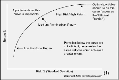
2.3 Efficient Frontier

The Efficient Frontier of Markowitz consists in a number of efficient portfolios, which are portfolios that have the highest return for a certain level of risk. Any portfolio below the EF can be considered to be inefficient, i.e., we should not invest on it. This concept appears with the question of what combination of assets

12

is the best one, considering that the inclusion of connections between assets returns and risk, leads to many potential good portfolios.

Some important assumptions we can clarify is that we can compose multiple portfolios, with one, two, or more combinations of N assets, so that all assets in the

portfolio are positively correlated, i.e., 0 < 𝜌_𝑖𝑗<1, for every combination of assets.

Figure 1: Efficient Frontier (http://financial-dictionary.thefreedictionary.com/Efficient+Frontier)

Assuming investors are risk averse, they prefer the portfolio that has the greatest expected return when choosing among portfolios that have the same standard deviation of return, also known as risk. Girard and Ferreira (2005) refer that the optimal portfolio along the EF is based considering the investor’s utility function and attitude towards risk. Those portfolios that have the greatest expected return for each level of risk describe the already explained EF, which coincides with the top portion of the minimum-variance frontier. On a risk vs. return graph, the portfolio with the lowest risk is known as the global minimum-variance (GMV)

13

portfolio, considering that for each level of expected portfolios return, we can vary the portfolios weights of the individual assets to determine the portfolio so called minimum-variance portfolios, i.e., the one with the lowest risk. A risk-averse investor would choose portfolios that are on the top of the EF because all available portfolios that are not on the frontier have lower expected returns than a portfolio with the same risk.

Portfolios above the curve are impossible and combinations below or to the right of the EF are dominated by more efficient portfolios along the frontier. The already known concept of diversification with new assets can allow us to expand the efficient frontier and add value, generating additional return in the portfolio at the same level of risk or reducing portfolio risk without sacrificing return.

There are many different techniques to deduce EF, like the single index model, developed by Bawa, Elton and Gruber (1979), that assume that the standard single index model is an accurate description of reality and allow investors to reach optimal solutions to portfolio problems. This model assumes that correlation between each security return is explained by a unique common factor that is the concerning index, i.e., we will combine the number of assets with one single index, for example, PSI20.

14

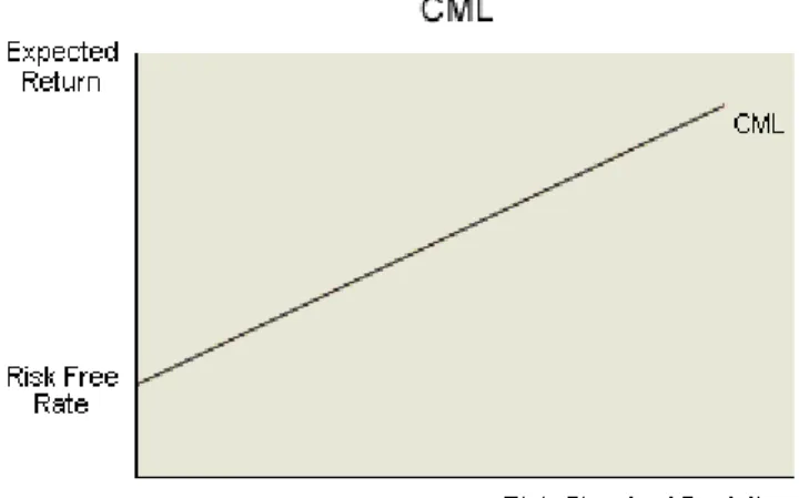
2.4 Capital Market Line and Separation Theorem

Tobin (1958) introduced the risk-free asset with the development of the Tobin Separation Theorem (TSB), together with the Capital Market Line model. According to TBS, an investor’s decision is made of two separate decisions: to be on the CML, where the investor initially decides to invest in the market portfolio, or according to their risk preference, leading the investor to a decision on whether to lend or to borrow at the risk-free rate in order to get the best portfolio. Buiter (2003) refers that the assumption behind TBS is that in a world with one safe asset and a large number of risky assets, the investor that is risk-averse, need to choose between them, being the weight between them determined by the degree of risk aversion of the investor. According to the level of risk aversion, with a well-diversified portfolio, investors will hold the market portfolio, because doesn’t exist a better portfolio in terms of risk. Dybvig and Ingersoll (1982) prove that TBS can only be obtained if all investors have quadratic utility, and that the relation can only hold if arbitrage opportunities exist in the market.

CML is based on the Capital Asset Pricing Model (CAPM) developed by Sharpe (1964) and Lintner (1965), which represents a linear relationship between return of individual assets and stock market returns over time, also called as a single-factor model, being considered as a general equilibrium model for portfolio analysis. It is a useful and used tool in order to describe the relation between risk and expected returns of individual assets, being acknowledged by the Nobel Price for William Sharpe in 1990.

15

We can check that the portfolios on the CML provide higher returns than the portfolios on the EF with the same risk level, meaning that the risk-free asset really helps the investor to reduce the risk of his portfolio, and also to preserve most of the return.

An important point is to differentiate the CML to the Security Market Line (SML). CML represents the allocation of capital between risk-free assets and a risky asset for all investors combined, and is based on EF, while SML is a trade-off between expected return and asset’s Beta. Resuming, we can define CML as a risk-return trade-off derived by combining the market portfolio with risk-free borrowing and lending, being all portfolios between the risk-free and the tangency point considered efficient.

Figure 2: Capital Market Line (http://www.investopedia.com/exam-guide/cfa-level-1/portfolio-management/capital-market-line.asp)

It’s represented by a linear function, where the slope is considered as the compensation in terms of expected return for each additional unit of risk and the

16

intercept point will be the risk-free. Since the expected return is a function of risk, CML can be represented by:

𝐸(𝑅_𝑝) = 𝑅_𝑓+𝐸(𝑅𝑀)−𝑅𝑓

𝜎𝑀 𝜎𝑝.

Thus, the expected return of any portfolio on the CML is equal to the sum of risk-free rate and risk premium, where the risk premium is the product of the market price of risk and the risk of portfolio under consideration.

2.5 Investor Profile

First of all, we assume that all investor are rational and have certain preferences over a chosen set of assets, which can be represented by a utility function. All consumers want to maximize their utility function subject to their budget constraint. The principle of rationality leads individuals to maximize their return, minimizing their expenses with the least possible risk. We can also apply the Pareto efficiency and the principle of equilibrium, where the prices adjust efficiently. Fama (1973) assume that the market is efficient, showing that the idiosyncratic risk does not affect prices, the prices adjust immediately to all available information, risk adjusted prices are not predictable, and that arbitrage opportunities are not present in financial markets.

Any investor would like to have the highest return possible from a certain investment. However, this has to be counterbalanced by the amount of risk that the

17

investor wants to take. It’s easy to assume that asset classes with bigger average return also have the highest risk.

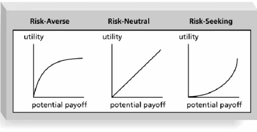
So the final decision in the determination of the optimal solution to the investor passes through maximizing their utility, which can be deducted through the indifference curves. And to understand the utility question, we can observe how utility functions and their properties work in terms of different investors’ profile. First of all, it’s important to assume the Von-Neumann Morgenstern Axioms (comparability, transitivity, strong independence, continuity, compose ranking and non-satiation).

Knowing this, the first utility function is consistent with the non-satiation

axiom, that says that an investor always prefer more to less, so 𝜕𝑈(𝑤)

𝜕𝑤 > 0, where 𝑤𝑖

concerns to wealth.

The second utility function studies the investor behavior towards risk, which can be studied through the second derivative in respect to wealth of the utility function. A risk-averse investor is the one that dislikes risk. For example, given two investments that have equal expected returns, this investor will hold risky assets if he feels that the extra return he expects to earn is sufficient in terms of

compensation for the additional risk. It’s represented by the function 𝜕2𝑈(𝑤)

𝜕𝑤2 < 0. We

can assume that the majority of the investors are risk-averse.

The risk-lover or risk-seeker is the one that prefers more risk to less and

given investments with equal expected return, will choose the riskier one, 𝜕

2_𝑈(𝑤) 𝜕𝑤2 >

18

0. Finally, a risk-neutral investor has no preference regarding risk and would be indifferent between two investments with the same expected return but different

risk, 𝜕2𝑈(𝑊)

𝜕𝑊2 = 0.

Figure 3: Risk Utility Function (http://m.yousearch.co/images/risk%20function)

2.6 Performance Measures

It’s important that, when in doubt of which portfolio to choose, we have some performance measures that allow us to rank the portfolios in order to be able to choose the best one. Jagric (2007) explain that, years ago, investors were almost exclusively interested in having great returns, but in the recent years, investors started to look to the assets and to the portfolio performance, what also leads to the risk performance consideration. These statistical measures include the Sharpe’s, Treynor’s and Jensen’s Ratio.

19

Levisauskait (2010) said that if a portfolio is well diversified, all these ratios/measures will agree on the ranking of the portfolios, because the well diversified total variance is equal to the risk of the market (β=1). In case this doesn’t happen, Treynor’s and Jensen’s measures can rank relatively undiversified portfolios much higher than the Sharpe Ratio does, because it uses both systematic and non-systematic risk.

2.6.1 Sharpe’s Ratio

Roy (1952) was the first to suggest a risk-to-reward ratio to evaluate a strategy’s performance and Sharpe (1966) introduced a measure for this performance analysis, applied to Markowitz’s mean-variance theory.

Dowd (2000) concluded that Sharpe’s ratio (SR) is a good measure because it gets both risk and return in a single measure, and for example, an increase in return differential or a fall in standard deviation leads to a rise in the measure and leads to a “good event”. When we have to choose between several alternative, SR lead to choose the one with the higher ratio measure. It can be measured by:

𝑆. 𝑅. =𝑅𝑝−𝑅𝑓

𝜎𝑝

A negative SR indicates that the risk-free asset would have a better performance that the actual portfolio.

20

We can also measure the performance by Treynor’s ratio (TR) (1965), which is a measure of excess return per unit of risk, i.e., compares the portfolio premium risk with the diversifiable risk of the portfolio measures by its Beta, or Jensen’s Alpha (Jα) (1967) that measure the performance of an investment as a deviation from this state of equilibrium, being based on CAPM, and measures the difference between an asset actual return and the return that could have been made on a benchmark portfolio with the same Beta.

2.7 Optimal Portfolio Selection

In 1973, Treynor and Black defended that to find the optimal selection in the active portfolio, only depends on the risk evaluation and not on market risk. The optimal portfolio of assets cannot be achieved with only human intuition and the behavior of a portfolio can be very different from the behavior of the individual assets on the portfolio.

Merton (1969,1973) prove that the portfolio-selection decision is independent of the consumption decision, which comes from the result of the assumptions of constant relative risk aversion and the stochastic process which generates the price changes, and of course that we can assume that the portfolio selection will always depend on the investor preferences.

In a general definition, the optimal portfolio is the one that, under market conditions and investor’s preferences, maximize his satisfaction or utility level. By

21

the expected utility theory, a risk adverse investor will never choose a non-efficient portfolio and there is always a portfolio that satisfies and maximizes the investors’ utility and an optimal portfolio for each one.

Elton et al. (1977) develop the single-index model in order to allow us to reach optimal solution to portfolio choice, and Bawa et al. (1979) added that short sales aren’t allowed and a riskless asset exists. These assumptions implied by the index model happen because the joint movements between securities have an association with the response of the market index and shows that the ranking procedure simplifies the computations necessary to determine an optimal portfolio.

The final optimal portfolio will be the one that combine the indifference curve with the capital market line. For example, portfolio 1 and portfolio 2 can both be optimal portfolios, but for different investors.

22

As we can observe, point P is the tangency point between the efficient frontier and the capital market line, which is also referred as the market portfolio. The optimal portfolio for each investor will be the highest indifference curve that is tangent to the capital market line that is the one with the greatest utility possible. We check that the first indifference curve concerns to a more risk-averse investor, while the second one concerns to a less risk-averse investor.

The combinations between the capital market line and the tangency point, allow us to reach different portfolios considering different percentages of risky assets and risk-free asset, and this depends therefore on the investor preferences in terms of the pretended return and the pretended risk.

23

3 Analysis of Portuguese Stock Index

The Portuguese Stock Index (PSI20) is the national benchmark index, constituted by the 20 biggest companies listed on Lisboa Stock Exchange. The liquidity of each listed company is measured by the transaction volume in the stock exchange. Actually, on the first week of May 2015, the PSI20 index “only” includes 18 listed companies (Altri, Banco BPI, BANIF, BCP, CTT, EDP, EDP Renováveis, GALP Energia, Impresa, Jerónimo Martins, Mota-Engil, NOS, Portucel, Portugal Telecom, REN, Semapa, Sonae SGPS and Teixeira Duarte).

Bartholdy and Mateus (2006), Allen and Gale (2000) conclude that Portugal is included in the group of bank-oriented countries with a universal bank system and strongly concentrated in a few financial groups, what means that the money flows essentially through financial institutions.

Banks or governments dominate as a source of finance, and financial reporting is aimed at creditor protection, what leads, regarding the existence of riskless market assets, to the consideration of the state financial instruments, like Treasury Bills. These ones are considered risk-free assets, because the default probability by the state is considered non-existent, considering also that, in case of a deficit, the government can get financial resources (taxes or banking) that allow paying the debt. In a general perspective, we consider Treasury Bills because they are the ones that work on a short term market, in terms of time horizon.

Financial reporting in stock markets is aimed as the information needed to outside investors. In terms of seasonal effects on the PSI20, Balbina and Martins

24

(2002) prove that the weekend effect tends to disappear in time with the evolution of the stock market. The Portuguese stock exchange works in 255 working days, since we don’t consider weekends and holidays.

Regarding the assumption of CML that we can lend and borrow money at the same risk-free rate, we just adopt the lending rate to estimate it, in spite of the existence of different borrowing and lending taxes.

Other important aspect to consider is the possibility of short sell. Short-selling is the practice of Short-selling securities or other financial instruments that are not currently owned. It’s important to understand that, even if the investor doesn’t have an asset, he can short sell, as if he actually has that same asset. What happens is that the financial institution that allow the short sell, borrow the assets required to another institution or, in some cases, that same institution borrow the necessary value to the investor.

In Portugal, these kinds of operations are regulated by Comissão de Mercado de Valores Mobiliários (CMVM). Analyzing the regulations under the CMVM rules, the short sale is allowed, but there are some restrictions to these operations. One of them concerns the short sale over financial institutions. CMVM,

in the instruction nº2/2008, clarifies that for the short sale be allowed, it’s

necessary that the investor has already some assets, at least at the same value to those he wants for short sale. Other obligation, it’s the duty of information of any short sale, as for example, the needs of the financial institution to guarantee the liquidity of the assets of their clients. These orientations can be found in Parecer

25 0 2000 4000 6000 8000 10000 12000 14000 16000 08 /05/2 000 08 /05/2 001 08 /05/2 002 08 /05/2 003 08 /05/2 004 08 /05/2 005 08 /0 5/ 2 00 6 08 /05/2 007 08 /05/2 008 08 /05/2 009 08 /05/2 010 08 /05/2 011 08 /05/2 012 08 /0 5/ 2 01 3 08 /05/2 014 08 /05/2 015

PSI20

Genérico sobre Vendas a Descoberto (Short Selling) of CMVM. So, considering all this regulations, we consider that in our case, it’s better to admit that we don’t allow short sell, to achieve a bigger number of potential investor and to simplify the achievement of the optimal portfolio.

The evolution of the Portuguese Stock Index in terms of price is represented by the graphic below.

26

4 Data Set and Methodology

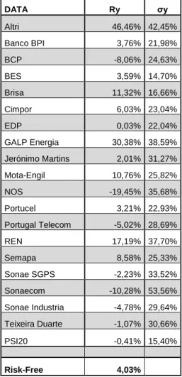
Historical data of stock market were taken from Datastream platform, from the first 2000 week to the first week of May 2015, divided in two different time periods, taking in consideration the objective of the work. The first period is from the first week of 2000 till the last week of 2008, and the second period is from the first week of 2009 till the first week of May 2015. As far as we know, doesn’t exist any study that allow us to know what is the ideal time period horizon to obtain a reliable input data (average return, standard deviation and covariance), so we consider a period between 5 to 10 years might be enough to reach conclusive results.

We consider as the risk-free interest rate for the calculations the EURIBOR rate for 1 year that has the average value of 3.025% on the first period and 0.169% on the second one. We are going to consider for the time horizon one year, so it can achieve an immediate investment for the actual civil year, considering all the calculated data in the first week of 2009 and May 2015, respectively.

On the first period 20 firms in PSI20 are represented, while in the second period 18 firms are represented in the PSI20 Index. The index represents the benchmark, and all the calculations are made in euros. The sample consists in 451 and 333 weekly observations, respectively.

The methodology of this work consists in the evaluation of the performance of the stocks (average rate of return, standard deviation and covariance), and the methods of construction of the EF and CML are presented. All the formulas will be

27

shown by the example of a certain company (for example, BPI) and the PSI20 will be used as benchmark.

The calculation of 1 week return of BPI is done as follows:

𝑅_{𝐵𝑃𝐼,1} = (𝑃𝐵𝑃𝐼,1−𝑃𝐵𝑃𝐼,0 𝑃𝐵𝑃𝐼,1 )

where: 𝑅_{𝐵𝑃𝐼,1} is the return of BPI in the first week;

𝑃_{𝐵𝑃𝐼,0} is the value of BPI in the beginning of the week;

𝑃𝐵𝑃𝐼,1 is the value of BPI in the end of the week.

The arithmetic mean of the return of the whole period is calculated as follows:

𝑅̅𝐵𝑃𝐼 =

∑𝑛_𝑖=1𝑅_𝐵𝑃𝐼

𝑛

where: n is the number of observations The variance of return of BPI is:

𝜎_𝐵𝑃𝐼2 =∑ (𝑅𝐵𝑃𝐼−𝑅̅𝐵𝑃𝐼)

𝑛 𝑖=1

2 𝑛−1

where: 𝜎_𝐵𝑃𝐼2 is the return variance of BPI.

The standard deviation is our representation of risk and is simply obtained

28 -60,00% -50,00% -40,00% -30,00% -20,00% -10,00% 0,00% 10,00% 20,00% 30,00% 40,00% 0,00% 20,00% 40,00% 60,00% 80,00% 100,00% 120,00% 140,00% Re tu rn Standard Deviation

Data Summary Pos 2009

Banco BPI BANIF BCP CTT EDP EDP Renováveis GALP Energia Impresa Jerónimo Martins Mota-Engil NOS Portucel Portugal Telecom REN Semapa Sonae SGPS Teixeira Duarte PSI20

Graph 2: Return vs. Risk (Post 2009 Period)

Calculations of returns and standard deviations are calculated using weekly

observations, but the results will be presented in values per annum, so, it’s

necessary to annualize the obtained values. Annualized return is obtained by:

𝑅_𝑦 = (𝑅_𝑤 + 1)52− 1

where: 𝑅_𝑦 is the annual return;

𝑅𝑤 is the weekly return.

In order to annualize the standard deviation of mean weekly return, it should

be multiplied by the squared root of the number of weeks in a year, so: 𝜎_{𝐵𝑃𝐼,𝑤} ×

√52.

We obtain the respective average annual returns and standard deviations for the two considered periods shown in the graphs below (complemented with figure 5 and 6 on appendix):

29

Graph 3: Return vs. Risk (Pre 2009 Period)

-30,00% -20,00% -10,00% 0,00% 10,00% 20,00% 30,00% 0,00% 10,00% 20,00% 30,00% 40,00% 50,00% 60,00% Re tu rn Standard Deviation

Data Summary Pre 2009

Banco BPI BCP BES Brisa Cimpor EDP EDP Renovaveis GALP Energia Jerónimo Martins Mota-Engil NOS Portucel Portugal Telecom REN Semapa Sonae SGPS Sonaecom Sonae Industria Teixeira Duarte PSI20

The formula of a covariance calculation between BPI and PSI20 is:

𝜎𝐵𝑃𝐼,𝑃𝑆𝐼20 = 1

𝑛∑ (𝑅𝐵𝑃𝐼− 𝑅̅𝐵𝑃𝐼)(𝑅𝑃𝑆𝐼20− 𝑅̅𝑃𝑆𝐼20) 𝑁

𝑖=1

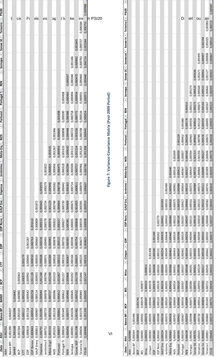
Considering the deduction of the variance and covariance, we use the data analysis function to construct the variance-covariance matrix that will later lead to the construction of the EF and CML. The results of the matrix are presented in the appendix (Figure 7 and 8).

30

4.1 Calculation of the Efficient Frontier

The objective of the optimal portfolio will be to minimize the total risk of the portfolio, which is obtained by the formula developed by Markowitz (1952):

𝜎𝑝2 = ∑ ∑ 𝑤𝑖𝑤𝑗𝜎𝑖𝑗 𝑛 𝑗=1 𝑖≠𝑗 𝑛 𝑖=1

where: 𝜎_𝑝2 is the variance of the portfolio;

𝑤_𝑖𝑎𝑛𝑑 𝑤_𝑗 are the weights of i and j assets in the portfolio;

𝜎𝑖𝑗 is the covariance between assets i and j.

In this work, we will assume some restrictions and constraints concerning the model developments and the Portuguese market. First of all, no borrowing or lending is allowed, so the objective will be to maximize the objective function𝜃 =

𝑅̅𝑝−𝑅𝑓

𝜎𝑝 , with the constraint∑ 𝑤𝑖

𝑛

𝑖=1 = 100%, because, taking the restriction into

consideration, the sum of all assets invested must be equal to 100%.

The complete return of a portfolio should be equal to the sum of the

weighted returns of the assets, so: ∑𝑛𝑖=1𝑤𝑖𝑅̅𝑖 = 𝑅̅𝑝.

We assume that the investors aren’t allowed to short-sell, which is reflected in the optimization by restricting all assets of having positive or zero investment,

so: 𝑤𝑖 ≥ 0, 𝑖 = 1, … , 𝑛. In order to avoid the complete domination of only one certain

31

restriction will be made. No asset may have more than 10% weight in the final

portfolio, so: 𝑤𝑖 ≤ 10%. This assumption is further specified in the results, with

evidences that without any restriction, efficient portfolios were just made by a simple stock.

Next, we use the Solver function to create several portfolios with different average return rates and risks, from the moment we achieve a minor portfolio return up to the moment of maximum possible return. This will lead to the construction of the efficient frontier, considering the connection between the returns and the standard deviation of the “solved” portfolios.

4.2 Calculation of the Capital Market Line

CML can be deducted beginning with the consideration of the formula:

𝐸(𝑅_𝑝) = 𝑅_𝑓+𝐸(𝑅𝑀)−𝑅𝑓

𝜎𝑀 𝜎𝑝.

The risk-free asset was already deducted and the second part of the formula represent the slope that lead to a linear function. As we already assume that no borrowing is allowed, our CML will be a line from the risk-free asset up to the point where the market portfolio is, and then we can consider through the investor preferences different combinations of these two types of assets.

32

5 Results

In this section, we present the results achieved for both periods.

Graph 4: Efficient Frontier (Pre and Post 2009 Periods)

Starting with the EF of Markowitz, we can observe a huge difference between the EF for the periods. We register that, in the period post 2009, the portfolio with 4,24% return is the so called GMV portfolio and that, from this one till the portfolios with higher returns, we acknowledge them as efficient portfolios. We don’t consider other portfolios because, for the measured level of risk, there exists always a portfolio with the same level of risk but a better level of return, that we call of inefficient portfolios. In the pre 2009 period, our GMV portfolio is the one with a

-4,00% -2,00% 0,00% 2,00% 4,00% 6,00% 8,00% 10,00% 12,00% 0,00% 1,00% 2,00% 3,00% 4,00% 5,00% R e tu rn Standard Deviation

Efficient Frontier

33

return of -3,28% that is a little bit influenced by the high risk-free asset that exist on that date.

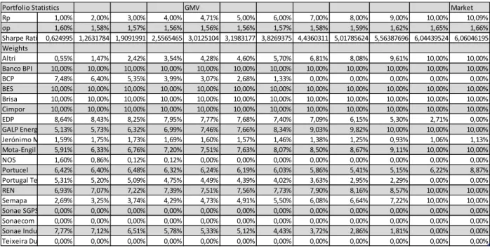
But we cannot forget that our final goal is to achieve the optimal portfolio, and to this we need to consider SR, that will work as our primarily performance measure. Our optimal portfolio, or the so called market portfolio, in our frontier will be the one with a return of 9,80%, on the post 2009 period, and 1,59% on the pre 2009 period, that are the ones with the higher SR.

Not considering the restriction assumed we will have 100% invested on CTT stocks, which will lead to a higher return, but also a higher risk. With the restrictions assumed, we were able to reduce the risk from 41,29% (risk of CTT stocks) to 3,72% through the process of diversification, in the post 2009 period. In this case, and assuming the maximum of 10% of each stock, we finalize with 10 different shares in the portfolio that allow us to diversify and, more importantly, reduce the risk. In the efficient frontier, we achieve a mean of 13 different stocks invested in the different portfolios, in both periods, what agrees with the proposition of a diversified portfolio.

Regarding CML, we achieve a linear function that goes from a return of 0,169%, that represents the risk-free asset, to the market portfolio, that have a return of 9,80% with 3,72% of risk, on the post 2009 period.

34

Graph 5: Capital Market Line (Pre and Post 2009 Periods)

In the pre 2009 period, we can see that we have a descendent line from 3,025% of return (risk-free rate) till the point with 1,59% return, which is the point that achieve the higher SR in that period.

All the points inherent to the line concerns to a certain combination between a risk-free asset and a risky asset, that in this case, is the market portfolio calculated above. We can check, for example, that if we invest 100% in the risk-free asset, we have 0,169% of return without go through any risk, and if we invest 100% in the market portfolio we have the return and risk already presented above. The investor can choose any combination on the line, with the perspective of more/less return regarding a possibility of more/less risk, what will lead us to the combination of the EF and CML.

0,000% 2,000% 4,000% 6,000% 8,000% 10,000% 12,000% 0% 1% 2% 3% 4% R e tu rn Standard Deviation

Capital Market Line

CML Post 2009 CML Pre 2009

35

Graph 6: EF and CML (Pre and Post 2009 Periods)

This last graph represents the combination of the two concepts developed in the work. As we can note again, the combination between the EF and the CML guarantees portfolios that have the same return but with less risk, in the aspect that instead of just investing in a portfolio with only risky assets, we can use the “optimal” portfolio and combine it with the risk-free asset to achieve a good return with a very low probability of risk.

In order to see the impact on the market of the 2008 crisis, we considered in addition the first period without the 2008 year, as shown in Figure 11 in the appendix. -4,00% -2,00% 0,00% 2,00% 4,00% 6,00% 8,00% 10,00% 12,00% 0,00% 1,00% 2,00% 3,00% 4,00% 5,00% Re tu rn Standard Deviation

Efficient Frontier and Capital Market Line

EF Post 2009 CML Post 2009 EF Pre 2009 CML Pre 2009

36

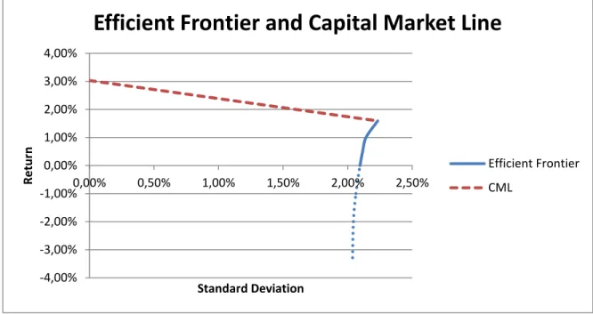
Graph 7: EF and CML (Pre 2008 and Pre 2009 Periods)

In this context, we can see that the year of 2008 is the real booster for the bad results obtained on this period. Disregarding that year, we go from a descendent CML to an ascendant one, and our maximum SR portfolio have a return of 10,09% with a risk of 1,66%. Another important difference is that we can achieve a positive (4,71%) GMV. -4,00% -2,00% 0,00% 2,00% 4,00% 6,00% 8,00% 10,00% 12,00% 0,00% 0,50% 1,00% 1,50% 2,00% 2,50% Re tu rn Standard Deviation

Efficient Frontier and Capital Market Line

EF (2000-2008) CML (2000-2008) EF (2000-2009) CML (2000-2009)

37

6 Conclusions

The concepts of EF and CML, in terms of financial studies and investment interests, have a great importance on the actual world. The study of these subjects, with the analysis of the Portuguese Stock Index, allows us to reach the efficiency or inefficiency of diversified portfolios and, at the same time, to understand the effect of 2008 Portuguese crisis on portfolios, considering the chosen time periods.

We can observe that, side by side, the two analyzed periods have huge differences between them.

Analyzing them separately, we can conclude that on the pre 2009 period the results achieved on the combination of the risky assets show us that we should invest 100% on the risk-free asset, what allow us to obtain a 3,025% return. This situation is odd surprising in the financial market framework, since the risk-free rate is above the PSI20 average return (-9,04%). On a posterior estimation, with the study of the period between 2000 and 2008, i.e., retrieving the year of 2008 from the data to test the same concepts but without the concern of the immediate effects of the crisis year, we can see that the year of 2008 is the real booster for the bad results obtained on that period.

On the second studied period, we achieved very different results in terms of the EF and, with a very low return on the risk-free asset, the optimal combinations should be the investment on more than 50% on the risky assets, what allow us to achieve returns superior to 5%, with a risk between the 2% and 3,5%. That should take us to bet on risky assets, and not only on the risk-free ones.

38

A rational investor would not be satisfied with a low return of 0,169% and, even without any risk, the investor must prefer to bet on risky assets considering that, with 3,72% of risk, the return achieved is near 10%. The slope, in the calculation of the SR, represents an incremental of 2,64 return considering the incremental risk.

After this analysis, we conclude that, after the crisis, the market was able to get back to better results, showing some recovery.

This work has the advantage to estimate the EF and CML as an instrument to portfolio investment decision, in the Portuguese case. However, this criteria is sensitive to the time spend, as shown for the first period, when the year of 2008 is not included in the first data. And so, this have some limitations, because we are also depending on the reliability of the input data when, for example, institutional investors want to use these models.

Further research should consider other periods and the impact that this might have on optimal portfolios, and the study with the same periods but in another market, to see the differences of the financial crisis between the Portuguese stock market and, for example, the Spanish or German stock market.

39

7 References

Allen, F., Gale, D. (2000), Financial Contagion. The Journal of Political Economy, Vol.108, Issue 1, pp.1-33.

Balbina, M., Martins, N.C. (2002), The Analysis of seasonal return anomalies in the Portuguese stock market. Banco de Portugal, Economic Research Department. Bawa, V., Elton, E.J., Gruber, M.J. (1979). Simple Rules for Optimal Portfolio Selection in a Stable Paretian Market. Journal of Finance, 34, nº2.

Banz, R.W. (1981), The relationship between return and market value of common stocks, Journal of Financial Economics 9, 3-18.

Bartholdy, J. and Mateus, C. (2005), ‘Debt and Taxes: Evidence from

Bank-Financed Small and Medium-Sized Firms’, Paper Presented at the 12th Annual

Conference of the Multinational Finance Society (Athens, Greece)

Brennan, T.J., Lo, A.W. (2011). The origin of behavior. Quarterly Journal of

Finance 1, 55-108.

Buiter, W.H. (2003), James Tobin: An appreciation of his contribution to economics. Economic Journal, Royal Economic Society, vol.113 (491).

Dowd, K (2000). Adjusting for risk: An improved Sharpe ratio. International Review

of Economics and Finance, 9, 209–222.

Dybvig, P.H., Ingersoll, J.E., (1982), Mean-Variance Theory in Complete Markets. The Journal of Business. Vol.55, nº2, pp.233-251.

40

Elton, E. J., Gruber, M. J. & Padberg, M. W. (1977), Simple Rules For Optimal Portfolio Selection: The Multi Group Case. Journal of Financial and Quantitative

Analysis, 329-345.

Elton, E. J., and Gruber, M.J. (1995), Modern Portfolio Theory and Investment Analysis, John Wiley & Sons Inc.

Fama, E. F. (1965), The Behavior of Stock Market Prices. Journal of Business, 37, January, pp. 34-105.

Fama, E. (1973). Risk, Return, and Equilibrium: Empirical Tests. The Journal of

Political Economy, 81(3), 607-636.

Fama, E.F. and French, K.R. (1992), The Cross-section of Expected Stock Returns. Journal of Finance, Vol. 47, No. 2, pp. 427-465.

Fama, E. F. & French, K. R. (1993), Common risk factors in the returns on stocks and bonds. Journal of Financial Economics, 33, 3-56.

Fama, E. & French, K. R. (2004). The Capital Asset Pricing Model: Theory and Evidence. Journal of Economic Perspectives, 18(3), 25–46.

Girard, E., and Ferreira, F. (2005), A n-assets efficient frontier guideline for investments courses, Journal of College Teaching & Learning 2(1), 53-65.

Gitman, L. J. (1997), Princípios de Administração Financeira. 7ª ed. São Paulo: Ed. Harbra.

Jagric, T., Podobnik, B., Stasek, S. & Jagric, V. (2007). Risk-adjusted Performance of Mutual Funds: Some Tests. South-Eastern Europe Journal of Economics, 2, 233-244.

41

Jensen, M. C. (1967), The Performance of Mutual Funds in the Period 1945-1964.

Journal of Finance, Vol. 23, No. 2, pp. 389-416.

Levišauskait, K. (2010). Investment Analysis and Portfolio Management. Leonardo

da Vinci programme project.

Lintner, J. (1965), The Valuation of Risk Assets and Selection of Risky Investments in Stock Portfolios and Capital Budgets. Review of Economics and Statistics, Vol. 47, pp. 13-37.

Marik, M. et al. (2007), Company Valuation Methods. Valuation Process – Basic

Methods and Procedures. 2nd _{ed. Prague: Ekopress.}

Markowitz, H. (1952), “Portfolio Selection”, The Journal of Finance, Vol. 7, Nº1, pp. 77-91.

Markowitz, H. (1959), “Portfolio Selection: Efficient Diversification of Investments”,

Cowles Foundation Monograph Nº16, New York: Wiley & Sons, Inc.

Markowitz, H. (1987). Mean-Variance Analysis in Portfolio Choice and Capital Markets. New York: Basil Blakwell.

Merton, R. C. (1969). Lifetime Portfolio Selection Under Uncertainty: The Continuous Time Case. Review of Economics and Statistics, 51, 247—257.

Merton R.C. (1973). An Intertemporal Capital Asset Pricing Model. Econometrica,

42

Roy, A. D. (1952), Safety First and the Holding of Assets. Econometrica, Vol. 20, No. 3, pp. 431-449.

Sharpe, W. F. (1964), Capital Asset Prices: A Theory of Market Equilibrium under Conditions of Risk. Journal of Finance, Vol. 19, pp. 425-442.

Sharpe, W. F. (1966), Mutual Fund Performance. Journal of Business, 39, pp. 119- 138.

Sharpe, W. F. (1975). The Sharpe ratio. The Journal of Portfolio Management. Sharpe, W. F. (1994). The Sharpe Ratio. The Journal of Portfolio Management,

Fall, 49– 58.

Tobin, James (1958), Liquidity preference as behavior towards risk. The Review of

Economic Studies, 25, pp. 65-86.

Treynor, J. L. (1965), How to Rate Managers of Investment Funds. Harvard

Business Review, 43, No. 1, pp. 63-75.

Treynor, J.L. and Black, F. (1973), How to Use Security Analysis to Improve Portfolio Selection, Journal of Business, 46, 66-86.

V Data Ry σy Altri 15,80% 34,22% Banco BPI -10,37% 46,77% BANIF -48,89% 132,26% BCP -26,38% 51,31% CTT 26,61% 41,29% EDP 1,73% 25,87% EDP Renováveis-0,60% 28,94% GALP Energia 3,04% 31,20% Impresa -9,29% 45,44% Jerónimo Martins14,86% 30,78% Mota-Engil -5,01% 42,88% NOS 4,31% 31,97% Portucel 13,76% 23,90% Portugal Telecom-37,73% 42,10% REN -1,52% 17,63% Semapa 8,13% 26,46% Sonae SGPS 12,71% 30,98% Teixeira Duarte-1,24% 58,51% PSI20 -2,94% 22,67% Risk-Free 0,169% Data Ry σy Altri 24,80% 45,54% Banco BPI -10,94% 27,89% BCP -20,60% 30,08% BES -7,61% 21,36% Brisa 1,62% 20,56% Cimpor -2,61% 27,06% EDP -7,07% 26,48% EDP Renovaveis 5,34% 37,95% GALP Energia 11,25% 42,00% Jerónimo Martins -3,61% 35,98% Mota-Engil -1,67% 29,21% NOS -26,93% 37,46% Portucel -2,91% 25,28% Portugal Telecom -9,64% 31,26% REN 10,80% 36,88% Semapa 3,21% 25,73% Sonae SGPS -18,20% 37,03% Sonaecom -22,10% 53,46% Sonae Industria -20,58% 33,77% Teixeira Duarte -16,74% 38,17% PSI20 -9,04% 18,90% Risk-Free 3,03%

Figure 5: Data Summary (Post 2009 Period)

Figure 6: Data Summary (Pre 2009 Period)

Efficient Frontier and Capital Market Line on PSI20 Daniel Bourdain VI D a ta A lt ri B an co B PI B A N IF B C P C TT ED P ED P R e n o vá ve isG A LP En e rg ia Im p re sa Je ró n im o M ar ti n s M o ta -E n gi l N O S Po rt u ce l Po rt u ga l T e le co m R EN Se m ap a So n ae S G PS Te ix e ir a D u ar tePS A ltr i 0, 00 22 52 B an co B P I 0, 00 13 90 0, 00 42 07 B A N IF 0, 00 01 68 0, 00 10 96 0, 03 36 41 B CP 0, 00 15 64 0, 00 31 65 0, 00 09 85 0, 00 50 63 CT T 0, 00 01 19 0, 00 01 17 0, 00 01 63 0, 00 03 75 0, 00 32 79 ED P 0, 00 08 18 0, 00 11 58 0, 00 00 42 0, 00 09 92 0, 00 00 43 0, 00 12 87 ED P R e n o vá ve is 0, 00 08 43 0, 00 09 54 0, 00 02 58 0, 00 11 39 0, 00 00 10 0, 00 07 63 0, 00 16 10 G A LP E n e rg ia0 ,0 00 81 3 0, 00 09 07 0, 00 01 14 - 0, 00 09 23 0, 00 00 33 - 0, 00 06 63 0, 00 08 09 0, 00 18 72 Imp re sa 0, 00 07 91 0, 00 10 85 0, 00 00 44 - 0, 00 12 48 0, 00 00 38 - 0, 00 05 36 0, 00 05 10 0, 00 04 43 0, 00 39 70 Je ró n imo M ar ti n s 0, 00 07 52 0, 00 07 19 0, 00 09 78 0, 00 07 96 0, 00 00 71 - 0, 00 04 93 0, 00 05 78 0, 00 07 24 0, 00 02 79 0, 00 18 22 M o ta -E n gi l 0, 00 15 10 0, 00 19 16 0, 00 07 27 0, 00 22 40 0, 00 02 84 0, 00 09 83 0, 00 09 74 0, 00 12 29 0, 00 09 46 0, 00 08 55 0, 00 35 35 N O S 0, 00 10 52 0, 00 13 18 0, 00 00 96 0, 00 14 19 0, 00 00 18 0, 00 08 78 0, 00 08 22 0, 00 07 48 0, 00 05 82 0, 00 04 56 0, 00 12 67 0, 00 19 66 P o rtu ce l 0, 00 08 37 0, 00 08 42 0, 00 04 12 0, 00 10 67 0, 00 01 52 0, 00 05 15 0, 00 05 57 0, 00 06 04 0, 00 07 38 0, 00 04 75 0, 00 09 59 0, 00 06 05 0, 00 10 98 P o rtu ga l T e le co m 0, 00 06 34 0, 00 14 45 0, 00 06 12 0, 00 11 57 0, 00 01 59 0, 00 07 35 0, 00 06 27 0, 00 07 30 0, 00 04 42 0, 00 03 18 0, 00 14 10 0, 00 08 98 0, 00 05 90 0, 00 34 08 R EN 0, 00 04 56 0, 00 07 57 0, 00 04 66 0, 00 08 06 0, 00 00 67 0, 00 03 65 0, 00 03 81 0, 00 04 09 0, 00 03 63 0, 00 02 89 0, 00 06 30 0, 00 04 48 0, 00 03 86 0, 00 04 66 0, 00 05 97 Se ma p a 0, 00 09 01 0, 00 10 36 0, 00 06 45 0, 00 10 32 0, 00 01 66 0, 00 05 96 0, 00 06 91 0, 00 06 75 0, 00 07 14 0, 00 05 00 0, 00 11 11 0, 00 07 23 0, 00 07 58 0, 00 04 94 0, 00 03 46 0, 00 13 46 So n ae S G P S 0, 00 11 98 0, 00 14 81 0, 00 05 32 0, 00 17 29 0, 00 00 25 - 0, 00 07 54 0, 00 08 58 0, 00 10 03 0, 00 08 15 0, 00 07 57 0, 00 15 24 0, 00 10 36 0, 00 07 75 0, 00 09 34 0, 00 04 70 0, 00 08 92 0, 00 18 45 Te ix e ir a D u ar te0, 00 06 56 0, 00 15 70 0, 00 08 45 0, 00 18 46 0, 00 02 25 0, 00 06 77 0, 00 05 59 0, 00 03 95 0, 00 09 79 0, 00 03 66 0, 00 12 63 0, 00 07 08 0, 00 05 34 0, 00 09 31 0, 00 04 60 0, 00 07 83 0, 00 07 37 0, 00 65 84 P SI 20 0, 00 09 90 0, 00 13 99 0, 00 04 95 0, 00 15 47 0, 00 01 01 0, 00 08 25 0, 00 08 38 0, 00 09 19 0, 00 06 07 0, 00 07 40 0, 00 13 08 0, 00 09 45 0, 00 06 54 0, 00 09 71 0, 00 04 40 0, 00 07 24 0, 00 10 44 0, 00 07 55 0, D a ta A lt ri B an co B PI B C P B ES B ri sa C im p o r ED P ED P R e n o va ve is G A LP En e rg ia Je ró n im o M ar ti n s M o ta -E n gi l N O S Po rt u ce l Po rt u ga l T e le co m R EN Se m ap a So n ae S G PS So n ae co m So n ae In d u st ri a Te ix e ir a D u ar tePS A ltr i 0, 00 39 89 B an co B P I 0, 00 02 64 0, 00 14 96 B CP 0, 00 05 30 0, 00 06 95 0, 00 17 41 B ES 0, 00 04 05 0, 00 05 82 0, 00 05 78 0, 00 08 77 B ri sa 0, 00 02 59 0, 00 03 74 0, 00 03 97 0, 00 03 33 0, 00 08 13 Ci mp o r 0, 00 05 83 0, 00 03 95 0, 00 04 46 0, 00 03 78 0, 00 03 14 0, 00 14 08 ED P 0, 00 04 89 0, 00 04 21 0, 00 06 15 0, 00 03 79 0, 00 04 38 0, 00 03 40 0, 00 13 49 ED P R e n o va ve is 0, 00 01 62 0, 00 02 88 0, 00 01 24 0, 00 01 30 0, 00 01 65 0, 00 01 31 0, 00 02 62 0, 00 27 70 G A LP E n e rg ia0, 00 02 54 0, 00 02 18 0, 00 03 66 0, 00 02 56 0, 00 02 84 0, 00 02 54 0, 00 04 29 0, 00 04 31 0, 00 33 93 Je ró n imo M ar ti n s 0, 00 05 00 0, 00 03 73 0, 00 05 29 0, 00 03 91 0, 00 02 93 0, 00 03 49 0, 00 06 48 0, 00 04 10 0, 00 05 33 0, 00 24 89 M o ta -E n gi l0 ,0 00 68 3 0, 00 04 26 0, 00 07 10 0, 00 04 50 0, 00 03 88 0, 00 04 63 0, 00 04 60 0, 00 00 80 0, 00 04 20 0, 00 05 07 0, 00 16 40 N O S 0, 00 04 29 0, 00 07 07 0, 00 06 93 0, 00 05 54 0, 00 03 51 0, 00 04 54 0, 00 05 39 0, 00 02 22 0, 00 02 75 0, 00 09 01 0, 00 05 18 0, 00 26 99 P o rtu ce l 0, 00 03 95 0, 00 04 31 0, 00 04 66 0, 00 03 20 0, 00 01 86 0, 00 02 47 0, 00 03 98 0, 00 01 26 0, 00 03 29 0, 00 04 80 0, 00 04 13 0, 00 05 59 0, 00 12 29 P o rtu ga l T e le co m 0, 00 01 93 0, 00 04 67 0, 00 05 56 0, 00 03 07 0, 00 03 37 0, 00 04 02 0, 00 05 29 0, 00 02 97 0, 00 04 27 0, 00 06 54 0, 00 03 67 0, 00 08 57 0, 00 04 52 0, 00 18 80 R EN 0, 00 02 38 0, 00 02 07 0, 00 00 89 0, 00 02 94 0, 00 01 68 0, 00 01 64 0, 00 02 54 0, 00 02 47 0, 00 04 64 0, 00 01 31 0, 00 02 27 0, 00 01 69 0, 00 02 45 0, 00 01 76 0, 00 26 15 Se ma p a 0, 00 02 82 0, 00 03 98 0, 00 04 71 0, 00 02 80 0, 00 02 91 0, 00 03 15 0, 00 03 49 0, 00 01 31 0, 00 01 92 0, 00 03 73 0, 00 04 29 0, 00 03 94 0, 00 04 63 0, 00 03 56 0, 00 01 13 0, 00 12 74 So n ae S G P S0 ,0 00 70 1 0, 00 09 46 0, 00 08 41 0, 00 07 51 0, 00 05 01 0, 00 05 05 0, 00 08 12 0, 00 01 45 0, 00 03 57 0, 00 09 84 0, 00 07 25 0, 00 13 13 0, 00 06 42 0, 00 09 10 0, 00 02 73 0, 00 05 20 0, 00 26 36 So n ae co m 0, 00 04 25 0, 00 07 36 0, 00 09 14 0, 00 05 53 0, 00 02 29 0, 00 04 99 0, 00 05 09 0, 00 00 19 - 0, 00 01 55 0, 00 05 73 0, 00 08 06 0, 00 13 56 0, 00 07 80 0, 00 12 18 0, 00 00 71 0, 00 05 68 0, 00 16 71 0, 00 54 95 So n ae In d u str ia 0, 00 08 30 0, 00 05 43 0, 00 06 04 0, 00 05 00 0, 00 03 17 0, 00 05 38 0, 00 05 43 0, 00 00 65 0, 00 02 32 0, 00 05 11 0, 00 06 89 0, 00 05 27 0, 00 05 36 0, 00 03 59 0, 00 01 64 0, 00 05 22 0, 00 09 54 0, 00 09 07 0, 00 21 94 Te ix e ir a D u ar te 0, 00 08 51 0, 00 08 60 0, 00 10 43 0, 00 07 12 0, 00 05 45 0, 00 06 42 0, 00 05 92 0, 00 00 48 - 0, 00 05 82 0, 00 07 41 0, 00 10 09 0, 00 06 46 0, 00 06 73 0, 00 04 95 0, 00 02 67 0, 00 06 42 0, 00 11 27 0, 00 09 08 0, 00 10 25 0, 00 28 02 P SI 20 0, 00 04 04 0, 00 05 70 0, 00 07 51 0, 00 04 59 0, 00 04 10 0, 00 04 22 0, 00 06 73 0, 00 02 37 0, 00 04 43 0, 00 06 50 0, 00 05 09 0, 00 07 76 0, 00 04 38 0, 00 08 20 0, 00 02 23 0, 00 03 93 0, 00 09 23 0, 00 08 67 0, 00 05 15 0, 00 07 25 Fi gu re 7 : V ar ian ce -C o var ian ce M atr ix ( Po st 2009 Pe ri o d ) Fi gu re 8 : V ari an ce -Co vari an ce M at ri x ( P re 2009 Per io d )