Contagion and regulation in endogenous bank networks

FUNDAC

¸ ˜

AO GET ´

ULIO VARGAS

ESCOLA DE ECONOMIA DE S ˜

AO PAULO

BERNARDO KEISERMAN

Contagion and Regulation in

Endogenous Bank Networks

FUNDAC

¸ ˜

AO GET ´

ULIO VARGAS

ESCOLA DE ECONOMIA DE S ˜

AO PAULO

BERNARDO KEISERMAN

Contagion and Regulation in

Endogenous Bank Networks

Disserta¸c˜ao apresentada `a Escola de Economia de S˜ao Paulo da Funda¸c˜ao Get´ulio Vargas, como requisito para a obten¸c˜ao do t´ıtulo de Mestre em Economia

´

Area do conhecimento: Macroeconomia

Orientador: Bernardo de Vasconcellos Guimar˜aes

Bernardo Keiserman

Contagion and Regulation in Endogenous

Bank Networks

Disserta¸c˜ao apresentada `a Escola de Economia de S˜ao Paulo da Funda¸c˜ao Get´ulio Vargas, como requisito para a obten¸c˜ao do t´ıtulo de Mestre em Economia

´

Area do conhecimento: Macroeconomia

Orientador: Bernardo de Vasconcellos Guimar˜aes

Data de aprova¸c˜ao:

26/03/2014

Banca Examinadora:

Prof. Dr. Bernardo de Vasconcellos Guimar˜aes

(Orientador) EESP-FGV

Prof. Dr. Bruno Ferman EESP-FGV

Agradecimentos

`

A minha fam´ılia, pelo apoio incondicional.

Ao Bernardo Guimar˜aes por todo apoio e orienta¸c˜ao.

Aos amigos da EESP e do PPGE, um dos grandes frutos do mestrado.

Aos amigos de Porto Alegre.

`

Abstract

We develop a simple model of endogenous bank networks to study financial con-tagion and how leverage regulation may affect it. Banks maximize expected profit by choosing the optimal allocation of resources between three different classes of assets. An interbank network arise as result of loans between banks, creating a direct channel of contagion in the financial system. Contagion may occur when the realized return of the risky asset is sufficiently low to make a bank insolvent, sub-sequently triggering a cascade effect that propagates through default in interbank loans. Contrary to what would be expected, our results show that despite forcing banks to deleverage, increasing minimum capital requirements may lead to a system with higher aggregate levels of default.

Resumo

Neste trabalho desenvolvemos um modelo simples de redes banc´arias end´ogenas para estudar cont´agio financeiro e como regula¸c˜oes de alavancagem podem afet´ a-lo. Bancos maximizam lucro esperado escolhendo a aloca¸c˜ao ´otima de recursos entre classes de ativos diferentes. Uma rede interbanc´aria surge como resultado dos empr´estimos realizados entre bancos, criando um canal direto de cont´agio no sistema. Cont´agio pode ocorrer quando o retorno realizado do ativo com risco for suficientemente baixo para deixar um banco insolvente, assim desencadeando um efeito cascata que se propaga atrav´es de defaults nos empr´estimos interbanc´arios. Ao contr´ario do que seria esperado, nossos resultados mostram que apesar de for¸car os bancos a desalavancarem, um aumento no n´ıvel m´ınimo de capital requerido pode levar a um sistema com n´ıvel agregado de default mais elevado.

Contents

1 Introduction 1

2 Literature Review 3

3 Model 5

4 Quantitative Analysis 11

5 Results 14

6 Final Remarks 19

1

1

Introduction

One of the main features of the recent financial crisis was the bankruptcy of Lehman Brothers, which immediately triggered a major cascade effect that spread out to the whole financial system and led to an unprecedented coordinated action among central banks as an attempt to stop financial contagion. These events shed light on the complex system structure of the banking activity nowadays and unraveled the dangers of contagion in such highly interconnected systems.1

This link between interconnectedness in banking systems and financial contagion motivated the study of financial networks, a strand of the literature that applies techniques commonly used in physics and biological sciences to economic network problems.

There has been a large developing literature on contagion in financial networks since the breakout of the crisis. Despite that, most works on financial contagion2

take the interbank network - which is obviously the core of any network problem - as an exogenous structure and focus the analysis on the spread of contagion in different network structures. Rather than assuming a random nature, it is reasonable to think that interbank networks arise as a result of banks’ optimizing behavior in a system where financial intermediaries are mutually known and have at least some information about each others risks.

To fill this gap, we propose a simple model in which financial linkages arise endoge-nously across optimizing banks, giving form to an interbank network in a flexible frame-work that allows the analysis of banks behavior in a range of scenarios and the conse-quences in terms of contagion. The importance of studying the structure of interbank connections stems not only from the fact that it has been directly linked to the stability of financial systems, but it also based much of the policy actions carried out after the crisis. In Basel III accord document (BIS, 2011, p.61) the Basel Committee states that ”one of the underlying features of the crisis was the build-up of excessive on- and off-balance sheet leverage in the banking system. In many cases, banks built up excessive leverage while still showing strong risk based capital ratios”. Thus, in the present work we focus our analysis in exploiting how regulation policies over banks leverage ratio limits affect the formation of interbank connections, and study conditions under which tighter regulation actually brings more instability to financial systems.

The model is basically structured in two parts. In the first part, banks maximize expected profit by choosing their investment allocation between three possible assets: risk-free bonds, a risky asset and loans. Financial regulation is introduced through a leverage restriction that constrains profit maximization by limiting banks’ assets to a multiple of its own endowed capital - it represents the leverage ratio limit introduced in Basel III. Interbank market interest rates are determined endogenously and reflect bank default probability as well as supply and demand of money. Loans established optimally

1

See Lo (2012) for a discussion about the growing interconnectivity in the financial system and the importance of its relation to the 2008 financial crisis, and Allen & Babus (2009) for a thorough review over the role of networks in modern financial systems.

2

2

by each bank define the financial network in our economy. The resulting allocation of funds in risky assets and bonds, together with interbank loans, compose the structure of the economy’s financial system. The second part of the model takes part once banks’ maximization is done and deals with financial contagion. When risky asset returns realize some banks may not be capable of honoring all debt, being forced to sell assets in a fire sale to keep solvency. The liquidation may trigger a defaulting cascade effect through the network. Financial contagion stops when withstanding banks are no longer affected by defaulting ones or when all banks fail.

In order to find an equilibrium to our model, we numerically solve a fixed point problem. The fixed point problem is composed by the following problems. The first one is to maximize bank’s expected profit by choosing portfolio allocations given prices -a risk-free interest r-ate, cle-aring interb-ank m-arket interest r-ates -and def-ault prob-abilities. Of course, loans depend on interest rates paid by banks in the interbank market, which in turn depend on their respective default probability. The second problem is to find default probabilities of banks given portfolio allocations and, specially, an interbank network. An equilibrium to our economy is achieved iterating these two problems until we find a fixed point.

3

2

Literature Review

The literature on contagion in financial systems is quite recent. It essentially began with the work by Allen & Gale (2000), the first to propose a model to explicitly study the relation between connections among banks and the resilience of the financial system.3

The model is built in a Diamond-Dybvig (1983) framework of banks and depositors with random liquidity preferences, and banks choice to invest in short and long term assets is crucial to avoid liquidity shortage. The approach to financial networks is made by introducing an interbank market where banks can exchange deposits as a form of insurance against preference shocks, while exposing the system to the risk of contagion. The authors show that complete structures, when banks are connected to all others, are more robust than incomplete systems since shocks are dispersed through a larger number of banks.

The externality effects of financial networks evidenced by the recent crisis exposed the necessity to better understand how network structures may affect system stability, so the literature had a great development since the breakout of the crisis. The work by Allen & Gale (2000) evolved to a strand of the literature that deals with network formation games; Babus (2009), Castiglionesi & Navarro (2010) and Cohen-Cole et al. (2013) are some examples of the works that apply game and graph theory techniques to analyze the formation of financial networks.4

While the basic modeling structure may differ, these works have in common the study of optimal financial networks - they try to understand how banks should connect to each other through an interbank market to reduce the risk of contagion and establish the most resilient system. The main contribution of these works is to refine the idea that more complete networks are more resilient to contagion. For example, Acemoglu, Ozdaglar & Salehi (2013) show that financial networks exhibit a ’robustyetfragile’ characteristic -the idea that -there exists a tipping point where more complete interconnections start to serve as a propagation mechanism rather than of absorbing the shocks.

At the other extreme of the literature are the works that assume an exogenous finan-cial network structure. Differently from the previously mentioned works, Gai, Haldane & Kapadia (2011) and Nier et al. (2007) take the interbank structure as given and focus the analysis on the potential spread of contagion rather than the probability of conta-gious default. Since these works don’t model agents behavior, they are able to construct networks as close as possible to reality.

Gai & Kapadia (2010) simulate aggregate and idiosyncratic shocks in arbitrary net-work structures to explore the impact in contagion and find the result later endorsed by Acemoglu et al. (2013) that financial systems exhibit a robust-yet-fragile tendency. Gai, Haldane & Kapadia (2011) extend the analysis and study how policies such as liquidity regulation and macro-prudential policy can reduce the spread of contagious default. How-ever, the network structure in these works is completely exogenous and, except for the

3

See also Freixas, Parigi & Rochet (2000).

4

4

randomness of shocks given in the system, the models are basically mechanical.

Our work is more related to the strand of the literature that attempts to combine the formal approach of optimizing agents with the analytic flexibility of exogenous networks. While the stylized approach of the former works fail to match the structures implied in real-world financial networks, by assuming the network structure as exogenous the latter models loose the capability to understand how policies affect the behavior of banks in the system. More specifically, our work is closely related to Bluhm, Faia & Krahnen (2013) and Georg (2013).

Georg (2013) builds a dynamic banking system model where banks update their port-folio according to liquidity demands (deposits fluctuate over time) and allocate funds in risky assets to maximize their utility. Technically his model is quite different from ours though, since interest rates are not endogenous and bank’s default probabilities do not affect the interbank market.

5

3

Model

3.1

Basic structure

The economy in our model is structured in three periods, t = 0,1,2, and agents in the economy are composed by i ∈ {1, ..., n} risk neutral financial intermediaries, henceforth

banks for simplification. Each bank i is endowed in t = 0 with deposits and owners’ capital,di andki respectively. Deposits and capital in each bank are definedex ante, and

together they comprise each bank initial funding.5

We also assume that both deposits and capital may differ across banks, and together with the return of the risky asset each bank may invest they establish banks heterogeneity.

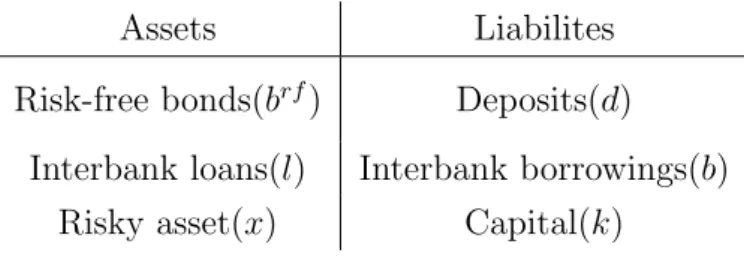
The balance sheet of each bank in the economy is similar to the structure adopted by Bluhm et. al (2013):

Table 1: Banks’ Balance Sheet

Assets Liabilites

Risk-free bonds(brf_{) Deposits(d)}

Interbank loans(l) Interbank borrowings(b) Risky asset(x) Capital(k)

As we can see from our simplified balance sheet above, there are three possible invest-ment vehicles for each bank: risk-free bonds, interbank loans and risky assets - or risky projects, as we alternatively use. The liabilities side of the balance sheet determines that the money to invest in those assets must come from banks’ initial funding, deposits and capital, and from interbank borrowing.

Each bank in the economy has the possibility to invest in a particular risky project at t = 1. Risky projects are investment opportunities available in the economy for each bank individually, and are not allowed for trading. The stochastic return of the project for bank i, θi, is given by two random components: a global one, common to all banks,

which is binary - high or low - and follows a Bernoulli distribution with parameterp, and a normally distributed idiosyncratic shock. The risky return is then given by:

θi =θ{H,L}+ǫi, ǫi ∼N(µi, σ 2

)

Note that the heterogeneity between banks may arise also among the risky return, whether with the stochastic disturbance of ǫi or with the predetermined average return, µi.

6

5

It is implicit from the predetermination of deposits and capital their exogeneity to bank’s optimization problem. Certainly, both deposits and capital play crucial roles in the bank industry and have been largely studied, specially by the bank runs and banks’ capital structure literature. Despite that, taking these into account is beyond the scope of this work.

6

6

We also specify a technology for banks investment in risky assets,xi. We assume that

xi have decreasing returns to scale, so that bank’sitotal return of investingxiunits in the

risky asset is given by xα_i.θi, whereα∈(0,1). Finally, at the final period, t= 2, projects

returns realize and banks collect profits or losses obtained by their respective risky assets. We return to portfolio composition when we define banks’ optimization problem in section 3.3.

3.2

The financial network

In our model the financial system is composed by i∈ {1, ..., n} banks, and an interbank market where banks may borrow and lend from each other. The borrowing connections that arise endogenously between banks in the interbank market configure our financial network structure.

Formally, in graph theory definition the network in our model is a directed weighted graph composed by n vertices or nodes, with each vertex corresponding to a bank, and where a link between vertices iand j is present if bank iis creditor - or debtor - to bank

j. The termdirectedrefers to fact that the link comprise both assets and liabilities, while

weighted refers to the value of the link between the two banks, i.e. the size of bilateral debt in monetary units.

Apart from financial regulation, we impose no exogenous constraints on how much banks can borrow from each other. Moreover, we model the interbank structure so as to allow banks for being creditors and debtors of others not only at the same time, but also being so of a particular bank at the same time. In other words, bank i may be a creditor and a debtor to bank j at the same time.7

That being said, borrowing links are formed endogenously by banks optimizing decisions, which in turn are constrained by accountability and leverage restrictions. We focus on this issue in the next subsection.

Suppose bank i is a debtor to bank j. Then, bi,j ∈ R denotes the quantity of

mon-etary units bank i borrowed from j. Thus, if bi,j = 0, it means that banks i, j are not

connected through the interbank market. Naturally, we can group all existing interbank connections into one n−squared adjacency matrix B, therefore simpliflying the whole network structure in one matrix. In that case, defining B as being a borrowing matrix, we have that each entry bi,j represents the quantity in monetary units bank i borrowed

from j and is such thatbi,j =lj,i, with lj,i denoting the loan of bank j to bank i.

Differently from most of the literature, in our model the interbank network do not only arise as a result of banks coinsurance or risk diversifying incentives, but rather over funds flowing to more efficient or profitable projects among the financial system.

economy. Firstly, the fact that each bank has only one possible risky asset to invest can be alternatively interpreted as a portfolio composed of a wide range of securities and investment vehicles, aggregated into one single product. Secondly, one can naturally think of the heterogeneity across risky assets average returns as, for example, banking managing efficiency translated into higher returns.

7

7

3.3

Banks’ optimization problem

Having defined the basic structure of the economy and characterized the financial network, we now proceed to specify the bank optimization problem. We model banks optimization as a profit maximization problem, given by the following equation:

max_brf

i ,bi,li,xiE(max{0, πi}) (1)

with

πi =xαi.θi+ (li.P(θ)).r+brfi .r rf _+k

i−bi.ri−di.rrf

where α is the decreasing returns to scale parameter, li = {li,j, ..., li,n} is the vector of

all loans made by bank i, P(θ) = {Pj(θ), ..., Pn(θ)} is the vector of realized interbank

repayments, i.e. the fraction of total borrowings each bank pays 8

, and is a function of the realized θ’s. The vectorr={rj, ..., rn}comprises the interest rate paid by each bank,

rrf _{is the risk-free interest rate, and b}

i = {bj,i, ..., bn,i} is the vector of all borrowings

made by bankiin the interbank market. We take the risk-free interest rate, rrf_{, as being}

exogenously given while r, the vector of interest rates paid by each bank in the interbank market, is determined endogenously in equilibrium through a market clearing mechanism. The vector of realized interbank repayments, P(θ), is determined endogenously and is directly connected to the default probability of each bank for a given network and an investment portfolio. In equilibrium, default probabilities reflect the average payments in the interbank market, or the average fraction of total borrowings each bank is capable of paying at the final period. By assuming that banks take into account the vector of paymentsP(θ), note that it makes implicit the fact that in equilibrium banks have perfect information about other banks’ risks. We return to P(θ) and explicitly define it in the next subsection.

Perhaps one of the main features of our model is in banks’ objective function. Dif-ferently from Bluhm et al. (2013) and Georg (2013), each bank in the system maximizes its expected net worth, subject to a limited liability condition that restricts bank net worth to zero. That is, in case of default, the maximum a bank can loose is its owners’ capital. The limited liability condition brings up moral hazard to the financial system by stimulating banks to take more risk since their losses are bounded at zero. Arguably, this moral hazard issue captured endogenously by our model revealed itself as a major problem among investment banks in the US after the financial crisis.

There are basically two constraints in the problem. The first one is a basic account-ability restriction: at t= 1, assets should equal liabilities, imposing that net assets equal net liabilities at the aggregate level in the economy. The second is a leverage constraint, representing the Basel accord capital requirements, which we shall call the Basel con-straint. Formally, banks are subject to the previously mentioned constraints and to the following non-negativity constraints:

8

8

xi+li+brfi =di +bi+ki (2)

ki ≥φ

xi+li+brfi

(3)

xi ≥0, brfi ≥0, li ≥0, bi ≥0 (4)

where φ ∈ (0,1) represents our key policy parameter, which we refer to throughout the text as the Basel parameter, once it defines the leverage ratio limit of all banks in the system.

The leverage ratio is a very important indicator of the riskiness a financial intermediary is exposed to as it relates the size of banks’ capital to its total assets. Since capital absorbs bank’s asset losses, the more equity a institution holds compared to its total assets, the higher is the buffer to possible losses. The Basel III agreement, elaborated in response to the recent financial crisis, introduced the minimum leverage ratio as a major requirement to prevent banks building up excessive exposure, as well as proposing to increase the quality of the capital buffer composition.9

The focus of the present work is to evaluate how leverage regulation may affect the stability of financial systems, so we perform simulations with different φ and analyze the consequences in terms of defaults.

3.4

Financial contagion

So far we have described that att= 0 the economy is composed byn banks, each endowed with deposits and capital, and how these banks solve their profit maximization problem by choosing the composition of their portfolio between three different assets: risk-free bonds, risky assets, and interbank obligations - loans and borrowings. Concerning the timing of the model, the maximization process occurs at t = 1, so that at t = 1 the interbank network is already placed, with all connections among banks defined with their respective interest rates, bi and ri, as well as the investment position of banks in risky

assets and risk-free bonds, xi and b rf i .

With all portfolio positions established, the dynamics in the economy continue to the final period. In t = 2, the stochastic returns of the risky assets realize and payment of interbank obligations should immediately take place, with banks finally remunerating depositors and profiting from their banking operations.

Now, suppose otherwise that the realization of θi, bank’s i risky asset return, is

suffi-ciently low such that bank i is not capable to honor all its debt obligations, but only a fractionPi(θ). In that way, financial contagion may occur in our model int= 2 depending

on the realization of risky assets returns. Specifically, we define the following solvency

9

9

condition10

:

ki +xαi.θi+ (li.P(θ)).r+b rf i .r

rf _−b

i.ri−di.rrf ≥0 (5)

that is, at t= 2 the bank should be capable of paying all its debt, or the net worth of the bank should be non-negative.

At this point, we make an assumption about the banks willingness to pay their own debt: banks will always honor their financial obligations as long as they are capable to, so choosing to partial ou total default is not an option. Since a bank that declares default on its obligations is very likely to suffer from a bank run or go under Central Bank intervention, for the purposes of the present work this is a quite plausible assumption to make.

Given that, if att = 2 a bank does not satisfy the solvency condition and is declared insolvent, we assume that the bank must sell all its assets at a liquidation cost λ ∈(0,1) in order to pay its creditors. The liquidation cost may be thought of as due to legal costs, asset illiquidity and fire sales, for example. Following the fire sale, the payment of the insolvent bank to its lenders is given by:

Pi(θ) =max

(

0,(ki+x

α

i.θi+ (li.P(θ)).r+brfi .rrf)(1−λ)−di

bi.ri

)

(6)

We also assume that depositors have seniority over other debtors, so that with the re-maining value obtained after the fire sale, the insolvent bank should first return depositors their principal. Depending on whether there is still some value left after honoring senior debtors, the fraction that the insolvent bank pays to others in the interbank market is defined by dividing the remaining value by the sum of all its interbank obligations remu-nerated according to its own interest rate. In case the defaulting bank have not enough money to pay its depositors, or if there is nothing left after depositors payout, then the bank collapses and is declared bankrupt, defaulting on all the banks it borrowed from in the interbank market.

In our model, insolvency may be initially triggered only by a low risky asset return, but it is propagated through financial contagion in the interbank market by the fire sale mechanism described above. This contagion mechanism is a direct propagation (or cascading) network effect, since an initially healthy bank may not be able to honor all its debt after receiving only a fraction of a loan payment or being totally defaulted by an insolvent bank. An equilibrium in the financial system, and consequently in the economy, is achieved when the cascading effects within the whole network stop.

The way we model financial contagion, the mechanism of payment adjustments works

10

10

as if all banking operations were made through a chamber of settlements whose job is to register negotiations and, when necessary, do the proper financial liquidation proceedings and payments across agents in the system. This is exactly the role played by stock exchanges in the case of securities and of central banks in the case of interbank obligations. The mechanism we use underestimates the cascade effect of contagion since it precludes over-the-counter operations, because they lack a centralized settlement institution and therefore difficult the simultaneous control of payments – e.g. that may lead to excessive margin calls.

11

4

Quantitative Analysis

In this section, we describe how do we solve the model numerically. Before doing that, first we need to define what is an equilibrium in our economy. An equilibrium in our model is composed by an interbank market, represented by the adjacency n-squared ma-trix B containing all borrowing links bi = {bi,j, ...bi,n}, ..., bn = {bn,i, ..., bn,j}, a vector

of investment in risky assets, x = {xi, ...xn}, a vector of investment in risk-free bonds,

brf _={brf

i , ..., brfn }, a vector of interbank interest rates, r={ri, ..., rn}, and finally a vector

of payments P(θ) = {Pi(θ), ..., Pn(θ)} that is a function of the realized θ = {θi, ..., θn}.

The payments vector P is a function of θ since each bank i maximizes profit for a given stream of θi and each realization of its risky return is related to the othersθj through the

global return component θ{H,L}.

In order to find an equilibrium to the economy, we basically need to solve a fixed point problem composed by two problems. The first one is to find a vector of payments P(θ) for a given set ofB,x,brf _{andr. The second is the reverse problem: for a given payments}

vector P(θ), we need to find a set of B, xand brf _{that maximizes banks’ expected profit}

under a market clearing interbank interest rate vector r. Therefore, an equilibrium is a fixed point achieved after the iteration of these two problems.

4.1

Maximization round

We begin our numerical approach by the second problem described above, the expected profit maximization of banks. For an underlying set of parameters and input variables, a given vector of paymentsP(θ) and a fixed vector of interest ratesr, banks maximize their expected profits by choosing the optimum allocation of funds over a drawn sequence11

of risky asset returns {θi, ..., θn}, according to the objective function (1) and subject to

constraints (2), (3) and the non-negativity constraints. That is, each bank in the network

simultaneously chooses how much to invest in the risky asset and the risk-free bonds, and how much it is going to lend and borrow from other banks through the interbank market. We call each maximization process above a maximization round. Note that banks’ profit maximization comprises a fixed point problem itself since interbank market clearing is achieved by adjusting portfolios and interest rates.

Here our approach importantly differs from our literature peers by the way the inter-bank linkages arise. Within each maximization round, a inter-bank chooses specifically which banks it wants to lend, as each bank pays its own interest rate for its borrowings and has its own default probability. On the other hand, a bank chooses the overall amount it wants to borrow, as for the borrower no matter from whom he borrows he is going to pay his own interest rate, and that is all he cares about.

At the end of each maximization round, although we have a set of optimumB,x, and

11

We draw a sequence of sufficiently large sizeN with (θi, ..., θn)) in each draw. In our simulations we

12

brf_{, the amount bank iis willing borrow, b}

i, may differ from the amount the other banks

in the network are willing to lend to bank i, which is given by Pn

j=1lj,i. Obviously, the

interbank market must clear in our equilibrium economy. To fix that we create a simple mechanism that adjusts interest rates according to excess supply or demand of funds.

At the end of each maximization round, we take Pn

j=1lj,i and bi and if the difference

between these two values is above some tolerance level for one or more banks, we proceed to interest rate adjustment. If not, the rate is kept unaltered. Suppose that at the of a maximization round there is excess demand for funds for bank i, i.e. bi ≥ Pn_j=1lj,i. In

this case, we take the excess demand value and add it to the current interest rate ri, so

that borrowing is more expensive to bank i and more attractive to other banks when we run the next portfolio optimization. In the opposite case when Pn

j=1lj,i ≥bi, we do the

reverse operation, subtracting the difference from ri.

We do the operation described above for every bank and then run a new maximization round, with banks optimizing using the updated interest rate vector and keeping all other variables constant. This iterative process continues until the difference between the supply and demand of funds for each bank is driven to a sufficiently low threshold, which leads to interbank market clearing.

With the resulting equilibrium in supply and demand of funds, it is possible to establish the adjacency matrix B by making bi = P

n

j=1bi,j =

Pn

j=1lj,i, that gives rise to the

interbank network structure in our model. This is important: network linkages among specific banks arise in our model as the result of their optimizing behavior, not randomly drawn across banks.

4.2

Contagion round

Once an equilibrium in the portfolio maximization of banks along with an interbank clearing market is reached, the payments vector P(θ) must be updated. Given B, x, brf

and r obtained in the step above we apply the solvency condition described before by equation (5) for each {θi, ..., θn} of the sequence initially drawn. Initially, every bank in

the network calculates his own profit supposing full repayment of lendings, i.e. Pi(θ) =

...=Pn(θ) = 1.

Now suppose that for one particular θi drawn of the sequence banki does not satisfy

the solvency condition. Then, as we described in section 3.4, bank i must apply equation (6):

Pi(θ) =max

( 0,(x

α

i.θi + (li.P(θ)).r+brfi .rrf)(1−λ)−di

bi.ri

)

13

each insolvent bank uses the remaining value to pay a fractionPifor each initialbi,j held. 12

This way the insolvency is, at first, spread immediately to the banks directly connected by the interbank linkages. At a second stage, all banks recalculate their solvency condition with the updated vector P(θ), which may trigger new insolvencies and so forth. This iterative process of financial contagion continues until the updating of P(θ) stops.

The process above is applied for every{θi, ..., θn} of the sequence initially drawn, and

for each we obtain a vector P(θ). The average of P(θ) is then used as the equilibrium vector of interbank payments to the underlying set ofB,x,brf _{andr, which is subsequently}

applied, updated, to the profit maximization step starting the whole process all over again. The process stops when changes in the equilibrium set reached between iterations are below a sufficiently low level.13

12

Note that insolvent banks are not excluded from the network when they go bankrupt, in the sense that banks that are debtors to an insolvent bank continue to have the same debt amount in the balance sheet.

13

14

5

Results

In this section we present the results from our simulations and show that a tighter leverage regulation may lead to a more instable financial system, an outcome that goes in the opposite direction desired by the policies recently implemented. The instrument of our analysis is the leverage ratio limit parameter, or Basel parameter, described before.

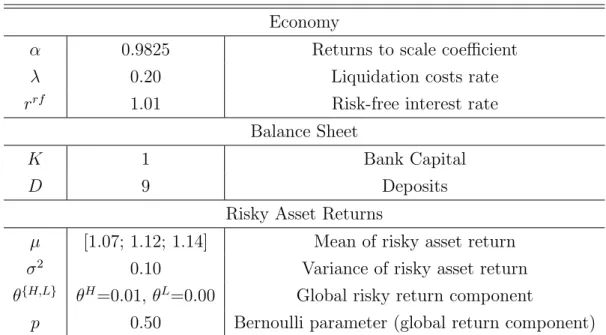
To run the simulations, we use a simplified system with only three banks. Capital and deposits are kept homogeneous across the network, therefore all banks have the same initial size in relation to the market. The heterogeneity within the system is given by the mean of the risky asset return particular to bank i, µi. The main parameters of

our baseline economy are the following: µ = (µA=1.07, µB=1.12, µC=1.14), σ 2

= 0.10,

λ = 0.20, K = 1 and D= 9.14

The other parameters can are in the table below:

Table 2: Baseline Parameters

Economy

α 0.9825 Returns to scale coefficient

λ 0.20 Liquidation costs rate

rrf 1.01 Risk-free interest rate

Balance Sheet

K 1 Bank Capital

D 9 Deposits

Risky Asset Returns

µ [1.07; 1.12; 1.14] Mean of risky asset return

σ2

0.10 Variance of risky asset return

θ{H,L} θH=0.01,θL=0.00 Global risky return component

p 0.50 Bernoulli parameter (global return component)

Keeping all other parameters constant, we vary the Basel parameterφthrough a range of values and check the default rates for each equilibrium outcome. We start by setting

φ = 0.086, to further decrease the leverage limit (increase φ) until the point where banks leverage allowance equals total funding amount, i.e. K

φ = (K+D) - in our case, φ= 0.10.

At this point the interbank network is inexistent since banks are not allowed to leverage beyond initial funds and therefore have no reason to borrow.

14

15

5.1

Baseline simulations

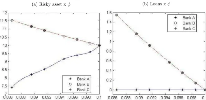
The figures below summarize the equilibrium portfolios in our baseline model for the three banks as we increase the level of capital requirement. Figure 1a shows the evolution of investment in the risky asset. Banks B and C, the more profitable ones, are fully leveraged and invested in the risky asset since the lower bound of φ, while bank A starts investing about 75% of its funding in the risky asset and increase this fraction untilφ = 0.10, when it is no longer able to lend money. Figure 1b shows the borrowing established in the interbank market. It is easy to see that it follows the movement described in figure 1a: as the leverage ratio limit is decreased, banks B and C leverage constraints are binding so they are forced to deleverage, so the amount borrowed decreases until the point where they ar unable to leverage and thus to borrow.

Figure 1: Portfolio evolution

(a) Risky asset xφ (b) Loans xφ

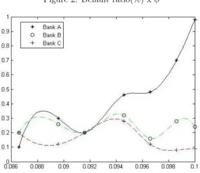
Figure 2 below illustrates the results from our simulations. It shows the default ratio (vertical axis), defined as the average (partial or total) default of each bank in equilibrium, for each level of capital requirement φ. While the default ratios from banks B and C are stable as the capital requirements are raised, bank A ratio significantly increases reaching a maximum of 1% default ratio when φ=0.10 and the interbank network is dried up.

Our model captures two distinct effects in the equilibrium system as the leverage ratio limit is altered. Firstly, we have the usual expected effect: as financial regulation gets looser, banks leverage up to invest in the risky assets and the overall exposure to risk in the system is increased. However, when φ is increased the model captures an unexpected increase in aggregate default ratio, although the overall exposure to risk is lower.

16

Figure 2: Default ratio(%) x φ

(in relation to other banks in the system) bank wants to lend because the return of the loans - adjusted by default probabilities - is higher than its own risky return. So as the leverage ratio limit is lowered (higher φ), and the leverage limit is binding, both efficient and inefficient banks get restricted in equilibrium through the limited interbank market. With the interbank market restricted, the more efficient banks are forced to deleverage - in relation to the unrestricted optimal risky asset investment - and the less efficient bank must reallocate loan funds between risk-free bonds or the risky asset. The latter gets prejudiced in two ways by the restriction. Firstly, as the other banks are forced to deleverage, the inefficient one needs to reallocate the resources in less profitable operations. Second, as the loans are reduced the bank portfolio is also less diversified, increasing its exposure to risk.

As the limited liability condition implied in the maximization objective function pushes the less efficient bank to invest more in its risky asset, the result is that its default probability increases significantly. In the limit, when φ is high enough to limit banks portfolio to their own initial funding, the inefficient bank invest all its funding in the risky asset and the default probability is potentialized. Finally, at the aggregate level the default risk also increase because the shorter exposure of efficient banks to risk is insufficient to overcome the consequences to the inefficient one. In equilibrium the bank with lower average return have its default risk increased significantly and, more than that, the resulting financial system is one with more defaults in average.

5.2

Robustness analysis

Now we use alternative parameters to simulate our model and check how the results behave in comparison to the baseline parameters.15

We begin varying the amplitude of

15

17

the difference in risky asset average returns across banks and compare the results in two regulation scenarios: with a ”looser” regulation and with the extreme scenario where there is no interbank market (φ= 0.10).

Table 3: Alternative µ µ= [1.07; 1.10; 1.12]

X B Default Ratio(%)

φ= 0.0866 [6.5887; 11.5469; 11.5473] [0; 1.5469; 1.5473] [0.62; 1.68; 0.92]

φ= 0.10 [10; 10; 10] [0; 0; 0] [1.04; 0.4; 0.2]

µ= [1.07; 1.16; 1.18]

X B Default Ratio(%)

φ= 0.0866 [6.5947; 11.5473; 11.5473] [0; 1.5473; 1.5473] [0.14; 0.26; 0.22]

φ= 0.10 [10; 10; 10] [0; 0; 0] [0.95; 0.07; 0.03]

As we can see from the table above, when we decrease the difference between banks’ average risky returns by setting µ = [1.07; 1.10; 1.12], the default ratios increase signif-icantly in comparison to our baseline model - both when φ = 0.0866 and φ = 0.10. Comparing the φ scenarios, we can still verify the effect of the forced deleverage: bank A has its default ratio increased while banks B and C ratio decreases. However, in this setting the aggregate default ratio decreases when the interbank market is inexistent. In the case where the amplitude between average risky returns is wider, the same pattern of the baseline setting is observed. When φ = 0.0866 default ratios are very close, with bank A being the least defaulting bank. On the other hand, when we set φ = 0.10 bank A’s default ratio becomes six times higher, and the aggregate default ratio is significantly increased.

Now we simulate the model using alternative variance of the risky asset return:

Table 4: Alternative σ2

σ2

= 0.08

X B Default Ratio(%)

φ= 0.0866 [6.5007; 11.5473; 11.5473] [0; 1.5473; 1.5473] [0; 0.06; 0.06]

φ= 0.10 [10; 10; 10] [0; 0; 0] [0.09; 0.02; 0.01]

σ2

= 0.115

X B Default Ratio(%)

φ= 0.0866 [6.5882; 11.5473; 11.5473] [0; 1.5473; 1.5473] [0.82; 2.04; 1.30]

18

From the simulation usingσ2

= 0.08 we again observe a pattern similar to our baseline model. Here, bank A departs from a situation with zero defaults to be the most defaulting bank in the system, when φ = 0.0866 and φ = 0.10 respectively. However, the aggregate default ratio is unaltered. When we set σ2

19

6

Final Remarks

We proposed a simple model of financial contagion where banks maximize expected profit by choosing the optimal allocation of resources between three different assets: risk-free bonds, risky assets and loans. An interbank network arises endogenously as result of loans between banks, creating a direct channel of contagion in the financial system. Contagion may occur when the realized return of the risky asset is sufficiently low to make a bank insolvent, subsequently triggering a cascade effect that propagates through default in interbank loans.

In this work we focused the analysis in the effects of regulation over banks’ leverage ratio, motivated by the Basel Committee proposals to introduce a leverage limit. We simulate our model in a simplified system of three banks for a range of leverage ratio limits and show that the average default rate may increase when banks are forced to deleverage, contrary to what would be expected. The bank with the lowest average returns has its default ratio significantly increased, moving from the position of less defaulting to most defaulting bank on average.

20

References

[1] Allen, F., Babus, A., 2009. Networks in finance, in: Network-based Strategies and Competencies. Edited by Paul Kleindorfer and Jerry Wind, Wharton School Publish-ing.

[2] Allen, F., Carletti, E., 2013. Deposits and bank capital structure. European University Institute Working Paper, ECO 2013/03.

[3] Allen, F., Gale, D., 2000. Financial contagion. Journal of Political Economy, 108(1), 1-33.

[4] Allen, F., Babus, A., Carletti, E., 2012. Asset commonality, debt maturity and sys-temic risk. Journal of Financial Economics, 104, 519-534.

[5] Acemoglu, D., Ozdaglar, A., Tahbaz-Salehi, A., 2013. Systemic risk and stability in financial networks. NBER Working Papers no.18727.

[6] Anand, K., Gai, P., Marsili, M., 2012. Rollover risk, network structure and systemic financial crises. Journal of Economic Dynamics and Control, 36, 1088-1100.

[7] Babus, A., 2007. The formation of financial networks. FEEM Working Paper no.69.

[8] Basel III: A global regulatory framework for more resilient banks and banking systems. Basel Committee on Banking Supervision, Bank for International Settlements, 2011.

[9] Bluhm, M., Faia, E., Krahnen, J. P., 2013. Endogenous banks’ networks, cascades and systemic risk. SAFE Working Paper no.12.

[10] Castiglionesi, F., Navarro, N., 2010. Optimal fragile financial networks. Working Paper.

[11] Cohen-Cole, E., Patacchini, E., Zenou, Y., 2012. Systemic risk and network formation in the interbank market. Working Paper.

[12] Diamond, D., Dybvig, P., 1983. Bank runs, deposit insurance and liquidity. Journal of Political Economy, 91(3), 401-419.

[13] Elliot, M., Golub, B., Jackson, M., 2013. Financial networks and contagion. Working Paper.

[14] Freixas, X., Parigi, B., Rochet, J., 2000. Systemic risk, interbank relations, and liquidity provision by the Central Bank. Journal of Credit, Money and Banking, 32(3), 612-631.

21

[16] Gai, P., Haldane, A., Kapadia, S., 2011. Complexity, concentration and contagion. Journal of Monetary Economics 58, 453-470.

[17] Georg, CP., 2013. The effect of the interbank network structure on contagion and common shocks. Journal of Banking and Finance, 37, 2216-2228.

[18] Gropp, R., Heider, F., 2009. The determinants of bank capital structure. European Central Bank Working Paper Series no.1096.

[19] Haldane, A., 2009. Rethinking the financial network. Speech delivered at the Finan-cial Student Association, Amsterdam. Available online.

[20] James, C., 1991. The losses realized in bank failures. Journal of Finance, 46(4), 1223-1242.

[21] Leitner, Y., 2005. Financial Networks: contagion, commitment, and private sector bailouts. Journal of Finance, 60(6), 2925-2953.

[22] Lo, A., 2011. Complexity, concentration and contagion: a comment. Journal of Mon-etary Economics 58, 471-479.