Sérgio Jorge Pereira da Costa

(1)

Sérgio Jorge Pereira da Costa

M.Sc.

Multi-Agent Model Predictive Control for

Transport Phenomena Processes

Dissertação para obtenção do Grau de Doutor em Engenharia Química e Bioquímica

Orientadores: José Paulo Barbosa Mota, Prof. Catedrático,

FCT - Universidade Nova de Lisboa

José Manuel P. V. C. Igreja, Prof. Coordenador,

ISEL - IPLisboa

Júri:

Presidente: Doutora Maria Adelaide de Almeida Pedro de Jesus

Arguentes: Doutor Nuno Manuel Clemente de Oliveira

Doutora Carla Isabel Costa Pinheiro

Vogais: Doutor José Paulo Barbosa Mota

Doutor João Fernando Pereira Gomes

Doutor José Manuel Prista do Valle Cardoso Igreja Doutor Francisco Avelino da Silva Freitas

(2)

(3)

Multi-Agent Model Predictive Control for Transport Phenomena Processes

Copyright cSérgio Jorge Pereira da Costa, Faculdade de Ciências e Tecnologia, Universi-dade Nova de Lisboa

(4)

(5)

(6)

(7)

A

CKNOWLEDGEMENTS

First of all I would like to thank my two supervisors, Professor José Manuel Igreja and Professor Paulo Mota.

Professor José Igreja for being my friend and my mentor for almost twenty years. My passion on control and mathematical systems came from him and from his enthusiasm. He has been present in every step of my growth as a person and a professional. This work and this thesis is also due to his tenacity and his involvement in every step of the way.

Professor Paulo Mota was the first person with whom I have made contact in Faculdade de Ciência e Tecnologia of Universidade Nova de Lisboa and almost immediately took me under his supervision. Outstanding person, helped me to overcome all obstacles and made everything possible for me to be presenting this work.

A special thanks to Professor João Miranda Lemos from Instituto Superior Técnico, for giving me the opportunity not only to keep on learning about control, but also for giving me permission to use some of his field data on experimental water delivery canal control as a means of validation of my work.

To the Chemical Engineering Departmental Area and Instituto Superior de Engenharia de Lisboa, for providing me the time and opportunity to keep evolving on my personal and institutional enrichment.

I also would like to thank all my colleagues, especially my friend Filipe for encouraging me almost on a daily basis, even when he was finishing his own. A word of appreciation to Valério for his kind words and for his encouragement all the time.

To my parents, my brother and his family for all the love, for all understanding and all the guidance. Without them everything would be much harder and thankfully they were always there for me.

Finally, for the two most important people of my life: my wife Patrícia and my daughter Maria. All the sleepless nights, all the nerves and all the setbacks were overcome with their dedication, their patience and, most of all, their love. Maria was born during the time I have been working on this thesis and I have to thank her for bringing me back to earth and for making me love her every gesture, every word and every care and affection. All of this couldn’t have been made without them.

(8)

(9)

A

BSTRACT

Throughout the last decades, control systems theory has thrived, promoting new areas of development, especially for chemical and biological process engineering. Production processes are becoming more and more complex and researchers, academics and industry professionals dedicate more time in order to keep up-to-date with the increasing complex-ity and nonlinearcomplex-ity. Developing control architectures and incorporating novel control techniques as a way to overcome optimization problems is the main focus for all people involved.

Nonlinear Model Predictive Control (NMPC) has been one of the main responses from academia for the exponential growth of process complexity and fast growing scale. Prediction algorithms are the response to manage closed-loop stability and optimize results. Adaptation mechanisms are nowadays seen as a natural extension of prediction methodologies in order to tackle uncertainty in distributed parameter systems (DPS), governed by partial differential equations (PDE). Parameters observers and Lyapunov adaptation laws are also tools for the systems in study.

Stability and stabilization conditions, being implicitly or explicitly incorporated in the NMPC formulation, by means of pointwise min-norm techniques, are also being used and combined as a way to improve control performance, robustness and reduce computational effort or maintain it low, without degrading control action.

With the above assumptions, centralized (or single agent) or decentralized and dis-tributed Model Predictive Control (MPC) architectures (also called multi-agent) have been applied to a series of nonlinear distributed parameters systems with transport phenomena, such as bioreactors, water delivery canals and heat exchangers to show the importance and success of these control techniques.

Keywords: Distributed parameters systems, nonlinear model predictive control,

(10)

(11)

R

ESUMO

Ao longo das últimas décadas, a teoria de controlo de sistemas tem prosperado, promovendo novas áreas de investigação e desenvolvimento, em especial no domínio da engenharia química e biológica. O aumento da complexidade e não linearidade nos processos produtivos faz com que investigadores, académicos e profissionais da indústria tenham de dedicar mais tempo ao seu estudo. O desenvolvimento de novas técnicas e arquiteturas de controlo tem ganho preponderância face aos problemas de optimização destes mesmos processos e o foco de atenção para todos os envolvidos.

O controlo preditivo não linear (NMPC) tem sido uma das principais respostas da investigação face ao crescimento exponencial da complexidade dos processos de produção e do aumento de escala dos mesmos. Os algoritmos de predição fazem face à garantia de estabilidade em malha fechada e na optimização dos resultados obtidos. Os mecanismos de adaptação começam a ser vistos como uma extensão natural das metodologias preditivas e são usados para resolver a incerteza associada aos sistemas de pârametros distríbuidos (DPS), compostos por conjuntos de equações diferenciais parciais (PDE). Observadores e mecanismos adaptativos baseados são utilizados para os sistemas aqui apresentados.

Estabilização e condições de estabilidade, implicita ou explicitamente incorporadas na formulação geral do NMPC como controlo do tipo pointwise min-norm, são usadas e combinadas com outras estruturas de forma a melhorar o desempenho, garantir a robustez e manter o esforço computacional baixo.

Tendo como ponto de partida as permissas acima indicadas, foram usadas estruturas de controlo centralizado (ou de agente único) ou controlo descentralizado ou, ainda, dis-tríbuído (controlo multi agente) em sistemas de pârametros distríbuidos com fenómenos de transporte, como sejam bioreactores, canais de distribuição de água ou permutadores de calor por forma a mostrar a importância e o sucesso destas técnicas de controlo.

Palavras-chave: Sistemas de pârametros distribuídos, controlo preditivo não linear,

(12)

(13)

C

ONTENTS

Contents xiii

List of Figures xv

List of Tables xxi

1 Introduction 1

1.1 Motivation . . . 1

1.2 State of the Art . . . 2

1.2.1 Operators and Semigroups . . . 2

1.2.2 Galerkin Method . . . 3

1.2.3 Orthogonal Collocation Method . . . 5

1.2.4 Flat Systems . . . 7

1.3 Model Predictive Control Architectures . . . 8

1.3.1 Single Agent or Centralized Control . . . 9

1.3.2 Multi-Agent Control . . . 9

1.4 Thesis structure . . . 12

2 Nonlinear Model Predictive Control in Bioreactors 15 2.1 Introduction . . . 15

2.2 Class of PDE models . . . 17

2.3 Process System Engineering design assumptions . . . 17

2.4 Stability . . . 18

2.5 Proposed NMPC general formulation . . . 20

2.6 Adaptive Control . . . 22

2.7 Application to a Fixed-Bed Tubular Bioreactor with Contois Kinetics . . . 23

2.7.1 Simulation run 1: Constrained/Unconstrained controller . . . 24

2.7.2 Simulation run 2: Input weight . . . 24

2.7.3 Simulation run 3: Additive disturbance . . . 26

2.7.4 Simulation run 4: Prediction horizon . . . 28

2.8 Conclusions . . . 31

(14)

CONTENTS

3.2 Finite Escape Traveling Time Distributed System . . . 34

3.3 Application to a Water Distribution Canal Pool . . . 38

3.3.1 Centralized Pointwise Min-Norm Control . . . 39

3.3.2 Fully Decentralized Pointwise Min-Norm Control . . . 42

4 Distributed Model Predictive Control for serially connected systems 51 4.1 Introduction . . . 51

4.2 Distributed Stabilizing Input/Output Receding Horizon Control . . . 53

4.2.1 Serially connected systems solution . . . 56

4.3 Parallel Iterated Solution . . . 57

4.4 Nominal Closed-Loop Stability . . . 58

4.5 Stability analysis without full iteration . . . 60

4.6 Water delivery canal . . . 63

4.7 Conclusion . . . 65

5 Model Predictive Control of Countercurrent Tubular Heat Exchangers with composite geometry 67 5.1 Introduction . . . 67

5.2 Prototype Model . . . 67

5.3 NMPC Nominal Formulation and Adaptive Control . . . 69

5.3.1 Adaptation with parameters observer . . . 70

5.3.2 Countercurrent Heat Exchanger Model . . . 71

5.3.3 NMPC combination with LAL dynamics . . . 73

5.4 Simulation results . . . 73

5.4.1 Centralized control . . . 74

5.4.2 Non-cooperative Distributed control . . . 82

6 Conclusions and Future Work 93 Bibliography 97 A Appendix 107 A.1 Pseudocode Algorithms . . . 107

A.2 Fixed-Bed Bioreactor routines . . . 107

A.3 Water Delivery Canal Pools . . . 113

A.4 Countercurrent Heat Exchanger . . . 118

(15)

L

IST OF

F

IGURES

1.1 Genealogy of MPC algorithms as seen in [97]. . . 1

1.2 Centralized Model Predictive Control architecture. . . 9

1.3 Decentralized Model Predictive Control architecture. . . 10

1.4 Distributed Model Predictive Control architecture. . . 11

1.5 Sequential Distributed Model Predictive Control architecture. . . 11

1.6 Parallel Distributed Model Predictive Control architecture. . . 12

2.1 Sets. . . 18

2.2 Simulation 1: Velocity (input) with stability constraint (black) and without (blue) 25 2.3 Simulation 1: Substrate (output) with stability constraint (black) and without (blue) . . . 25

2.4 Simulation 1: Parameters estimation . . . 26

2.5 Substrate and substrate estimator:S(t),Sa(t). With stability constraint (black) and without (blue) . . . 26

2.6 Simulation 1: Biomass,X(t), and biomass estimator,Xa(t), with stability con-straint (black) and without (blue) . . . 27

2.7 Simulation 1: Control Lyapunov Function with stability constraint (black) and without (blue) . . . 27

2.8 Simulation 2: Output,s(1,t), with (black) and without (blue) stability condition. 28 2.9 Simulation 2: Velocity (input) with (black) and without (blue) stability condition. 28 2.10 Simulation 2: Control Lyapunov function,V(t), decreasing (black) andV(t)/10 without stability condition (blue) oscillating. . . 29

2.11 Simulation 2: Substrate and Subtract estimation, with (black) and without (blue) stability condition. . . 29

2.12 Simulation 1: Biomass and Biomass estimation, with (black) and without (blue) stability condition. . . 30

2.13 Simulation 3: Output,s(1,t). . . 30

2.14 Simulation 3: Velocity (input) . . . 30

(16)

LIST OFFIGURES

2.16 Output: s(1,t). Solid line represents higher prediction horizon and dashed line represents lower prediction horizon. Dash-dot and double dotted lines

represent intermediate horizons. . . 31

2.17 Velocity (input). Solid line represents higher prediction horizon and dashed line represents lower prediction horizon. Dash-dot and double dotted lines represent intermediate horizons. . . 32

2.18 Lyapunov function:V(t)Solid line represents higher prediction horizon and dashed line represents lower prediction horizon. Dash-dot and double dotted lines represent intermediate horizons. . . 32

3.1 Numerical solution, 200 finite differences, for u=2.5m/s,θ =2 andx(z, 0) =1 36 3.2 Statex(z,t)transition, forθ =2,α=2 andφ=0.0001. . . 37

3.3 Manipulated velocityu[m/s]. . . 37

3.4 Robust statex(z,t)transition, forθ ∈[1.8 2.2],α=2 andφ=0.0001. . . 38

3.5 Manipulated velocityu[m/s]. . . 38

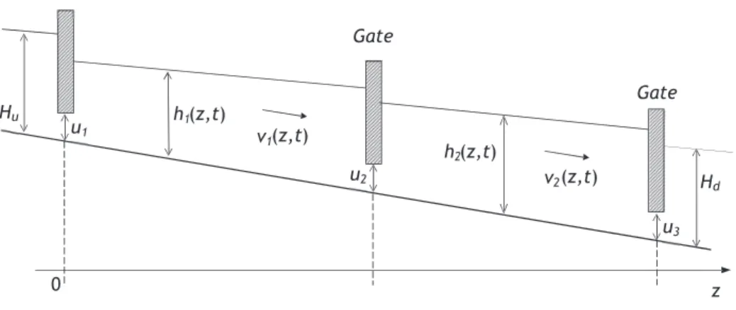
3.6 Canal pool schematic. . . 39

3.7 Frictionless water oscillation in a closed single pool. . . 40

3.8 Water elevationh(z,t) [m]with real Manning coefficient of 0.018 (concrete canal). 40 3.9 Water elevationh(z,t) [m]for a Manning coefficient of 0.1 . . . 41

3.10 Centralized Robust PointWise Min-Norm (RPWMN) scheme: Water elevation h(z,t) [m]for simulation run 1. Manning coefficient of 1. . . 41

3.11 Centralized RPWMN scheme: Water velocityv(z,t)[m/s] for simulation 1. . 42

3.12 Centralized RPWMN scheme: Upstream gate openingu[m] for simulation 1. 42 3.13 Centralized RPWMN scheme: Water elevationh(z,t) [m]for simulation 2. . . 43

3.14 Centralized RPWMN scheme: Upstream gate openingu[m] for simulation 2. 43 3.15 Two canal pools schematic. . . 44

3.16 Decentralized RPWMN scheme: Water elevation h1(z,t) [m](first pool) for simulation 1. . . 44

3.17 Decentralized RPWMN scheme: Water elevationh2(z,t) [m](second pool) for simulation 1. . . 45

3.18 Decentralized RPWMN scheme: Upstream gate openingu1 [m] for simulation 1. 45 3.19 Decentralized RPWMN scheme: Middle gate openingu2[m] for simulation 1. 45 3.20 Decentralized RPWMN scheme: Water elevation h1(z,t) [m](first pool) for simulation 2. . . 46

3.21 Decentralized RPWMN scheme: Water elevationh2(z,t) [m](second pool) for simulation 2. . . 46

3.22 Decentralized RPWMN scheme: Upstream gate openingu1[m] for simulation 2. 47 3.23 Decentralized RPWMN scheme: Middle gate openingu2[m] for simulation 2. 47 3.24 Decentralized RPWMN scheme: Water elevation h1(z,t) [m](first pool) for simulation 3. . . 47

(17)

LIST OFFIGURES

3.25 Decentralized RPWMN scheme: Water elevationh2(z,t) [m](second pool) for

simulation 3. . . 48

3.26 Decentralized RPWMN scheme: Upstream gate openingu1[m] for simulation 3. 48 3.27 Decentralized RPWMN scheme: Middle gate openingu2[m] for simulation 3. 48 4.1 Agent shared information service,Ci; Information interchanged by systemi, Σ_i, is depicted in the service bus.If(b)denotes forward (backward) interactions and thedidenotes disturbances. . . 54

4.2 SIORHC prediction horizon with contraints. . . 55

4.3 Example. . . 61

4.4 Example with the original algorithm. Cost functionk1 =0,k2=0.005. . . 61

4.5 Example with modified algorithm. Cost functionk1=0,k2 =0.005. . . 61

4.6 Three unstable serially connected systems; Outputs. . . 63

4.7 Three unstable serially connected systems; Inputs. . . 63

4.8 Normalized cost function; As predicted the cost function for the entire system is monotonically decreasing and therefore the system is asymptotically stable in closed-loop. . . 64

4.9 Control of a water delivery canal with Decentralized SIORHC [58] . . . 64

5.1 Sets with state reference curve level including real and nominal parameters. . 68

5.2 Prototype system: simple (top) and composite (bottom) geometries. . . 68

5.3 Prototype system: perspective composite geometry with countercurrent flows. Blue arrows and red arrows define cold and hot fluid flow, respectively. . . . 69

5.4 Parameters estimation: ˆa, ˆb[min−1]. . . 72

5.5 Parameters estimation for disturbed system: ˆa, ˆb[min−1]. . . 72

5.6 Simulation 1: Temperature tracking reference. Dotted lines mark both refer-ences; Cold fluid temperature (blue line with left-to-right direction marker) and hot fluid temperature (red line with right-to-left direction marker). . . 74

5.7 Simulation 1: Cold fluid temperature profile. . . 74

5.8 Simulation 1: Hot fluid temperature profile. . . 75

5.9 Simulation 1: Hot fluid velocity [m/min]. . . 75

5.10 Simulation 1: Robust control Lyapunov function. . . 75

(18)

LIST OFFIGURES

5.16 Simulation 3: Temperature tracking reference. Dotted lines mark both refer-ences; Cold fluid temperature (blue line with left-to-right direction marker)

and hot fluid temperature (red line with right-to-left direction marker). . . 78

5.24 Simulation 4: Hot and cold fluid velocity [m/min]. . . 81

(19)

LIST OFFIGURES

(20)

(21)

L

IST OF

T

ABLES

2.1 Bioreactor parameters. . . 24

2.2 Tuned RHC parameters. . . 24

2.3 Estimation and convergence parameters. . . 25

2.4 Tuned Receding Horizon Control (RHC) parameters for simulation 2. . . 27

2.5 Prediction horizon parameter for simulation 4. . . 29

3.1 Pool physical parameters. . . 40

5.1 Heat Exchanger parameters, initial and boundary conditions. . . 72

(22)

(23)

G

LOSSARY

CLF Control Lyapunov Function.

cMPC centralized MPC.

DMC Dynamic Matrix Control.

dMPC decentralized MPC.

DMPC distributed MPC.

DPS Distributed Parameter System.

dSIORHC decentralized SIORHC.

FLC Feedback Linearizing Control.

GPC Generalized Predictive Control.

ISS Input-to-State Stability.

LAL Lyapunov Adaptation Law.

MIMO Multiple Input Multiple Output.

MPC Model Predictive Control.

NMPC Nonlinear Model Predictive Control.

OC Orthogonal Collocation.

OCM Orthogonal Collocation method.

ODE Ordinary Differential Equaltion(s).

PDE Partial Differential Equation(s).

PSE Process System Engineering.

(24)

GLOSSARY

PWMNC PointWise Min-Norm Controller.

QP Quadratic Programming.

RCLF Robust Control Lyapunov Function.

RH Receding Horizon.

RHC Receding Horizon Control.

RLCF Robust Lyapunov Control Function.

RPWMN Robust PointWise Min-Norm.

SIORHC Stabilizing Input Output Receding Horizon Control.

SISO Single Input Single Output.

(25)

C

H

A

P

T

E

R

1

I

NTRODUCTION

1.1 Motivation

Over the last three to four decades MPC has been extensively studied and developed both in linear and nonlinear systems. MPC can be described as an optimization of the future behaviour of a process by using a model, making the model the basis of the controller. Rawlings presents in [100] an extensive survey focusing on the application of MPC using a very simple and straight forward language to introduce a set of complex terms, as well as presents a typical example regarding the usage of MPC. In [97] the authors focus on industrial application of MPC algorithms provided by vendors, reporting both linear and nonlinear applications, as depicted in 1.1.

LQG

IDCOM-M HIECON

SMCA

PCT PFC

IDCOM SMOC

Connoisseur

DMC DMC+

QDMC

RMPC RMPCT

1960 1970 1980 1990 2000

1st generation MPC 2nd generation

MPC 3rd generation

MPC 4th generation

MPC

Figure 1.1: Genealogy of MPC algorithms as seen in [97].

(26)

CHAPTER 1. INTRODUCTION

nonlinear systems are far less studied. Take notice that the nonlinearity in these processes is at least promoted by mass and energy conservation laws as well as chemical kinetics and its relationship with the properties of the final products.

1.2 State of the Art

When dealing with DPS several methods have been proposed in order to solve many of the challenges that these systems (especially the nonlinear) introduce. Many researchers and research groups developed mathematical solutions to deal with both linear and nonlinear systems (for instance parabolic or hyperbolic Partial Differential Equation(s) (PDE) systems) has it will be described below.

1.2.1 Operators and Semigroups

In [27] the authors start by motivating what they find has the usefulness of developing a theory for linear infinite dimensional systems and to do so they begin to present a series of control problems to practical and industrial applications. Their next step was to generalize the studied systems in the form:

˙

z= Az(t) +Bu(t),t≥0, z(0) =z0 (1.1)

whereZis a separable complex Hilbert space. In the example proposed, the authors

define the operatorsAandBas:

A = d

2

dx2

D(A) = _{z∈ L2(0, 1);Mz= M1(.)|0,1+M2d(.)

dx |0,1=0} (1.2)

B = I

and with Z = L2(0, 1)as the state space, z(·,t) = {z(x,t), 0 ≤ x ≤ 1}as the state,

u(_·,t)as the input andz0(·)∈ L2(0, 1)as the initial state. The boundary conditions,Mz,

are defined in the operator Adomain. After the formulation, the solution is obtained and given by:

z(x,t) = Z 1

0 g(t,x,y)z0(y)dy+

Z t

0

Z 1

0 g(t−s,x,y)u(y,s)dyds (1.3)

whereg(t,x,y)is given by:

g(t,x,y) =1+

∞

∑

n=0

2e−n2π2tcos(nπx)cos(nπy). (1.4)

A bounded operatorz(t) =T(t)z0onL2(0, 1)is then introduced in order to simplify

the above solution as:

z(x,t) =T(t)z0+

Z t

0 T(t−s)u(s)ds. (1.5)

(27)

1.2. STATE OF THE ART

This new bounded operator is what is called a strongly continuous semigroupas its

properties inT(t):R+_{→ L}(Z)are satisfied:

T(t+s) = T(t)T(s), for t,s _≥0; (1.6)

T(0) = I; (1.7)

kT(t)z0−z0k → 0, as t→0+ ∀z0∈ Z. (1.8)

In [32] the authors use a similar deduction for a parabolic PDE with boundary control actuation subject to input and state constraints.

1.2.2 Galerkin Method

One other approach on DPS control was suggested and developed in [11] and further ahead in [24], where the authors primarily describe hyperbolic and/or parabolic distributed systems such as, for instance heat exchangers, and use a different method from the one presented in the previous section in order to solve the set of PDEs. Although there are some differences in the adopted notation in both documents, the DPS can be written as:

∂v(t)

∂t = Av(t) +B f(t) (1.9)

with the initial conditions v(t) = v0 and output y(t) = Cv(t). The operator A is

described like in 1.2.1 and originates aC0semigroupU(t), with a growth property:

kU(t)_k≤Ke−σt, t ≥0, K≥1 and σ >0 (1.10)

andBandCoperators are defined as:

B f(t) =

M

∑

i=1

bifi(t) (1.11)

yj(t) = (cj,v(t)), 1≤ j≤ P. (1.12) with bothbiandcjbeing influence functions in the Hilbert spaceH. This DPS can be written as:

v(t) =U(t)v0+

Z t

0 U(t−τ)B f(τ)dτ, y(t) =Cv(t) (1.13)

as a weak formulation of the original DPS. A reduced-order model is then obtained:

∂vN

∂t = ANvN+ANRvR+BNf

(1.14)

∂vR

(28)

in order to synthesize a finite dimensional feedback controller using the Galerkin method.

In the latter, the author in [24] presents a similar DPS formulation:

∂x¯

∂t = A

∂x¯

∂z +B

∂2x¯

∂z2 +wb(z)u+ f(x¯)

yi = Z β

α c

i₍_z₎_k_xdz_¯ _, _i₌_{1, . . . ,}_l _(1.15)

qk = Z β

α s

k₍_z₎_ω_xdz_¯ _, _k₌_{1, . . . ,}_p

subject to the boundary conditions and initial condition, respectively:

C1x¯(α,t) +D1∂x¯

∂z(α,t) = R1 (1.16)

C2x¯(β,t) +D2∂x¯

∂z(β,t) = R2

¯

x(z, 0) = x¯0(z). (1.17)

In this formulation ¯x is the state, z and t are respectively space and time, α and β

are the domain of the process,u,yandqare, respectively, the manipulated inputs, the

controlled outputs and the measured outputs. The functions b(z), ci(z) and sk(z)are smooth functions ofz. This system can now be written as a infinite dimensional system in

Hilbert spaceH:

˙

x=_Ax+_Bu+ f(x), x(0) =x0

(1.18)

y= _Cx, q=_Qx

with:

Ax = A∂x¯

∂z +B

∂2x¯

∂z2 (1.19)

x∈ D(_A) = _{x∈ H([α,β];Rn); C1x¯(α,t) +D1∂x¯

∂z(α,t) = R1;

C2x¯(β,t) +D2∂x¯

∂z(β,t) =R2}

and

Bu = wbu

Cx = (c,kx) (1.20)

(29)

Like in the previous formulations,_Agenerates a strongly continuous semigroup if the eigenspectrum for_Acan be partitioned in finite-dimensional of slow eigenvalues and a stable infinite-dimensional complement of fast eigenvalues and that this separation between slow and fast is large [24]. With so, the general solution for the system can be written in the form:

x(t) =U(t)x0+

Z t

0 U(t−τ)[(Bu(τ) + f(x(τ))]dτ (1.21)

with:

kU(t)_{k ≤}K1ea1t, ∀t ≥0. (1.22)

Take notice that the formulations presented are very similar and the authors use the Galerkin approximation method to design the controllers and obtain the solution for these systems.

1.2.3 Orthogonal Collocation Method

As seen so far, the research in DPS applications is based upon different mathematical techniques. In [30] the authors describe a dynamical model for a fixed bed bioreactor in the form:

∂x1

∂t = K¯1ϕ¯(x1,x2) (1.23)

∂x2

∂t = F A

∂x2

∂z K¯2ϕ¯(x1,x2) (1.24)

with boundary conditions:

x2(t,z=0) =x2,in(t). (1.25)

In this dynamical modelx1andx2are the states,ϕ(x1,x2)is a function in(x1,x2)that

describe the kinetics, ¯K1, ¯K2andFare, respectively, the yield coefficient matrices and the

hydraulic flow rate. Finally,Ais the cross-section area of the bioreactor. The authors then

propose themselves to achieve a reduced model by using the Orthogonal Collocation method (OCM) [120]. With this method the PDEs are transformed into a series of Ordinary Differential Equaltion(s) (ODE) by expanding the variables as a finite sum of products of time and space functions:

x1(z,t) = p+1

∑

j=0

Bj(z)x1,j(t), x1,j(t) =x1,j(t,z=zj) (1.26)

x2(z,t) = p+1

∑

j=0

(30)

with Lagrange polynomials in the form:

βj(zi) =

(

1 if i= j

0 if i6= j . (1.28)

The reduced model can now be written as a set of ODEs in each collocation point and at the output:

dx1

dt = K1ϕ(x1,x2) (1.29)

dx2

dt = − F

ABx2+FR+K2ϕ(x1,x2) (1.30)

wherex1 and x2 are column vectors of states at each collocation point, ϕ(x1,x2)is

a column vector of the original ¯ϕ(x1,x2) also at the collocation points,K1 and K2 are

diagonal matrices of ¯K1and ¯K2, respectively andBij andFRare matrices that depend on the derivative ofβijalong space at the chosen collocation points (for further understanding please read [30]).

The resulting output will be obtained as:

dY dt =−

F AC

T_Bx

2+ F

AC

T

2b¯p+1x2,in+θTφ (1.31)

where Y is the value of the controlled component at the reactor output, yi is the concentration of the controlled component along the reactor at the collocation pointszi,

CTBx2is a linear combination of only the variablesyi at the different collocation points andθandφare column vectors of the unknown and known parameters, respectively.Fis the controlled input.

The stated advantages when implementing OCM, for instance when deducing an adaptive controller such as described [30], is that this method is by far easier when compared with the Galerkin method and also that after the model reduction the integrity and nature of the original system remains unchanged. Take note that the mass balances are preserved as demonstrated in [23].

In [50] we propose a similar application as in [30], but for a system modelled as:

∂w

∂t − u L

∂w

∂z = p(w,x,d) (1.32)

∂xk

∂t + vk

L

∂w

∂z = fk(w,x,d). (1.33)

In this case,wis the fluid temperature that circulates countercurrent on a jacket and xk are the state variables that represent the components for a given set of endothermic reactions in a inner tube (bothwandxkare space and time functions),u,vk andLare fluid and transport velocities and tube length, respectively.

The application of the OCM is identical to the one described earlier and, in this case, the objective is to control the space distributed output:

y(t) = 1 z2−z1

Z z₂

z1

xp(z,t)dz (1.34)

(31)

by manipulatingu(t)using an adaptive control scheme.

1.2.4 Flat Systems

One other major important mathematical technique for DPS is the concept of flatness and flat systems. Flatness appeared in a series of papers like [37, 38] and later on in [34, 72, 102, 103] and uses the formalism of differential algebra. The authors use this formalism to say that"a system is said to be flat if one can find a set of variables, called the flat outputs, such that the system is (non-differentially) algebraic over the differential field generated by the set of flat outputs"[84]. In a more simplistic definition, a system is flat if it exists a set of outputs in

the same number as the inputs, such that it is possible to obtain all states and inputs of a system from these outputs without the need for integration. This means that for any given system with statesx∈Rnand inputs_u_∈Rm then the system is flat if there are outputs

y∈Rm:

y=h

x,u, ˙u, ¨u, . . . ,(ur)

(1.35)

such that:

x = ϕ y, ˙y, ¨y, . . . ,

(q)

y !

(1.36)

u = α y, ˙y, ¨y, . . . ,

(q)

y !

. (1.37)

A very interesting use of flat systems in chemical engineering is the one published in [65]. In this paper, the authors define the system as a inhomogeneous parabolic DPS in the form:

α∂x(z,t)

∂t =−Ax(z,t) +u(z,t), z∈[0, 1, t>0] (1.38)

subject to the boundary conditions:

B1x(0,t) = w1(t), t >0 (1.39)

B2x(1,t) = w2(t), t >0 (1.40)

and initial conditions and control output, respectively, defined as:

x(z, 0) = x0(z), z∈[0, 1] (1.41)

y(t) = x(0,t), t ≥0. (1.42)

(32)

A(_·) , β2 ∂ 2

∂z2(·) +β1

∂

∂z(·) +β0(·) (1.43)

Bi(·) , Bi1 ∂

∂z(·) +Bi0(·), i=1, 2. (1.44)

The solution is then presented forx(z,t)as:

x(z,t) =

+∞

∑

i=0

ai(t)ϕi(z) = +∞

∑

i=0

ai(t)z i

i! (1.45)

and then approximated, assuming uniform convergence, by its firstN+1 terms:

x(z,t) =

N

∑

i=0

ai(t)

zi

i!. (1.46)

The same approximation can be performed on the control inputu(z,t):

u(z,t) =u(t)

m

∑

i=0

fiz i

i!, fi ∈R, f06=0, m≤N−2. (1.47)

The resulting model 1.38 is now written as:

α

N−2

∑

i=0

˙

ai(t)z i

i! +β2 N−2

∑

i=0

ai+2(t)z i

i! +β1 N−2

∑

i=0

ai+1(t)z i

i! +β0 N−2

∑

i=0

ai(t)z i

i! =u(t) m

∑

i=0

fiz i

i! (1.48) with boundary conditions 1.39 and output 1.41, respectively:

B11a1(t) +B10a0(t) = w1(t) (1.49) N−1

∑

i=0

1

i![B21ai+1(t) +B20ai(t)] = w2(t) (1.50)

y(t) =x(0,t) =

N

∑

i=0

ai(t) 0i

i! ≡ a0(t). (1.51)

This formulation is obtain by using the Power series solution of differential equations. One other study on flatness and flat systems is presented in [57] where the authors use flat systems theory and motion planning in order to solve an hyperbolic PDE system that describes a distributed collector solar field. Although taken into account the differ-ences between parabolic an hyperbolic systems, the application is similar to the one just described being the differences restricted to notation form.

1.3 Model Predictive Control Architectures

Now, the focus is to understand the main MPC architectures applied in various distributed parameters systems such as bioreactors, water canals and chromatography columns. Understanding the architecture and pointing out the differences and applications leads to a better knowledge on how different architectures were implemented and, in some cases, similar results were attained.

(33)

1.3. MODEL PREDICTIVE CONTROL ARCHITECTURES

1.3.1 Single Agent or Centralized Control

Centralized MPC (cMPC) as been a widespread control architecture over the last decades in different areas such as chemical and biological engineering [21, 30, 33, 52], power systems [91], supply chains [125], aerospace engineering [63] as well as energy efficiency for construction [123].

MPC

SYSTEM

Subsystem 1 Subsystem 2

u1 u₂

y₁ y₂

Figure 1.2: Centralized Model Predictive Control architecture.

Commonly applied to linear systems, as for instance in [17, 25], cMPC has suffered com-pelling advances in nonlinear systems theory and processes. It takes a single multivariable system and its interactions and uses one controller to compute all control actions [105]. By doing so, optimal solutions can be obtained by manipulating the inputs, minimiz-ing the difference between predicted and desired behaviour of a given system or set of subsystems.

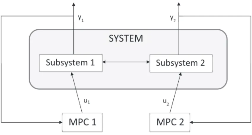
Figure 1.2 depicts a generic cMPC applied to a system containing two subsystems. Although of all the advantages in application to linear and low complexity systems, this centralized architecture generates more computer effort as the complexity and nonlinearity of the systems increase.

The evolution of MPC algorithm from a simple unconstrained Single Input Single Output (SISO) case using Dynamic Matrix Control (DMC) and Generalized Predictive Control (GPC) as described in [78] to nonlinear control systems [59, 81] with stability constraints, such as Stabilizing Input Output Receding Horizon Control (SIORHC) [48, 49] and/or with adaptation algorithms [51, 52, 53, 55, 56, 60] is thoroughly discussed in control systems theory literature.

1.3.2 Multi-Agent Control

1.3.2.1 Decentralized Model Predictive Control

(34)

used in different subsystems and treated as disjoint sets. These sets of inputs and outputs are coupled in a way that the resulting pairs do not overlap and the local controllers can then be designed to operate independently [105]. The decentralized framework has as main aspect the fact that the controllers inside a given system do not communicate with each other, which means that there is no information trading, although as seen in [47] information is exchanged only for special purposes.

SYSTEM

MPC 1 MPC 2

u1 u₂

y₁ y₂

Figure 1.3: Decentralized Model Predictive Control architecture.

In terms of stability analysis a great number of papers have been presented [6, 80, 116, 117, 124], giving particular relevance to the application of Input-to-State Stability (ISS) which was first introduced in [110] and further developed in [62, 98, 112] on nonlinear discrete-time systems or for constrained uncertain nonlinear systems [73].

1.3.2.2 Distributed Model Predictive Control

Contrariwise to dMPC, on distributed MPC (DMPC) [35] information is exchanged be-tween the controllers in order to have coordination in their actions. One of the major classes of DMPC are non-cooperative [75, 76] where the communication between con-trollers can be one-directional and the concon-trollers are evaluated in a sequence, Sequential DMPC, or at the same time, Parallel DMPC. The other class is cooperative DMPC [39, 69, 77, 90, 113] where the same global cost function is optimized in each controller. In the last decades several research developments have been achieved with the use of DMPC, namely advances in thermal and energy efficiency [12, 13, 14, 15] and for chemical engi-neering systems [87, 108, 115]. Recent design methods were developed to solve two major problems: guaranteeing stability and improving performance (please read [42, 64, 118]).

1.3.2.3 Non-cooperative DMPC

Like was said before, non-cooperative DMPC uses a set of local controllers whose actions are taken in order to optimize local cost functions. With this type of configuration there is no need for a given subsystem to know what happens, trajectory-wise in the other subsystems, including its neighbours. The exception is mostly focused in guaranteeing

(35)

1.3. MODEL PREDICTIVE CONTROL ARCHITECTURES

SYSTEM

MPC 1 MPC 2

u1 u₂

y₁ y₂

Figure 1.4: Distributed Model Predictive Control architecture.

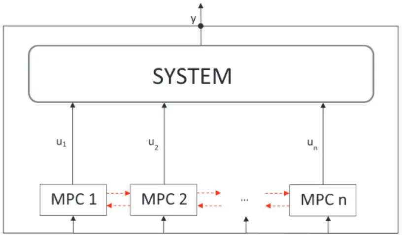
stability. In order to obtain some solution, at each sampling time, these controllers can exchange information only once (non-iterative parallel controllers) or can iterate (iterative parallel controllers). The iterative algorithms deal with a higher amount of information being exchanged, rather than non-iterative algorithms. Sequential and parallel designs are depicted in figures 1.5 and 1.6 respectively. Mathematical background for non-cooperative game theory can be read in [8].

SYSTEM

MPC1 MPC2 MPCn

u1 u₂ u_n

… y

Figure 1.5: Sequential Distributed Model Predictive Control architecture.

1.3.2.4 Cooperative DMPC

(36)

SYSTEM

MPC1 MPC2 MPCn

u1 u₂ u_n

…

y

Figure 1.6: Parallel Distributed Model Predictive Control architecture.

should be taken into account in suboptimal control theory. Interesting applications can be seen in [79].

1.4 Thesis structure

This thesis is, therefore, organized as follows:

• Chapter 1 includes a summary of the whole thesis, namely reports the main motiva-tion for the writing of this thesis, the state of the art in terms of the proposed work, different MPC architectures applied to nonlinear systems, including a brief descrip-tion of centralized, decentralized and distributed designs to be further developed and the organization of all chapters.

• Chapter 2 defines a general formulation for the class of uncertain nonlinear systems with transport phenomena proposed, introduces stability constrainment and applies receding horizon control with adaptation for a fixed-bed tubular bioreactor as an application of the given system.

• Chapter 3 extends the subjects presented in chapter 3 to other systems within the same class of distributed and uncertain nonlinear systems, namely to a finite es-cape traveling time distributed system. An application to a water delivery canal is thoroughly presented and discussed in SISO and Multiple Input Multiple Output (MIMO) cases with different control architectures, namely centralized and decentral-ized control.

• Chapter 4 is the extension of the previous chapter with the introduction of cooper-ative distributed control (multi-agent control) with zero state terminal constraints. New control techniques, mainly neighbour-to-neighbour cooperation have been applied to the water delivery canal prototype, as well as the developed generic serially chained systems solution.

(37)

1.4. THESIS STRUCTURE

• Chapter 5 makes use of assumptions and definitions from previous chapters and uses them as an application for a countercurrent heat exchanger. Centralized and non-cooperative distributed control techniques are developed and compared in terms of performance, robustness and computational effort.

(38)

(39)

C

H

A

P

T

E

R

2

N

ONLINEAR

M

ODEL

P

REDICTIVE

C

ONTROL IN

B

IOREACTORS

2.1 Introduction

In this chapter, the main goal is, first of all, to introduce the importance of NMPC in control systems theory and invoke some of the work that has been developed for this thesis as an application to a fixed bed tubular bioreactor.

Previously presented and developed for linear systems, in [36] and later on in [44, 99] NMPC has been proven to show important advantages in terms of advanced process control. This is due to the fact that constraint incorporation tends to be easier, becoming a decisive advantage for industrial applications when compared to other methods. The extension to multivariable cases can also be easier and well understood.

However, from an implementation standpoint, a major issue and main focus on re-search consists in being able to ensure stability for a short finite horizon in an uncertain environment, without dramatically increasing the computational effort. Usually, when in presence of uncertainty in a already complex nonlinear system, closed-loop stability has been shown to be extremely hard to achieve. The solution for these problems is the use of larger weight penalty on control action included in the optimization problem or bigger finite horizon in the controller, which tends to transform the optimization into higher computational effort. From a practical perspective, closed-loop stability is not decisive, and therefore many MPC techniques applied in process industries do not meet this feature. However, as can be read in [107] stability is convenient.

(40)

CHAPTER 2. NONLINEAR MODEL PREDICTIVE CONTROL IN BIOREACTORS

to be developed in this chapter and further on in chapter 3) will guarantee robust NMPC closed-loop stability. A stable distributed parameter estimator, in the Lyapunov sense, is also to be presented when combined with the NMPC algorithm, using the certainty equivalence principle for adaptation proposes.

Notwithstanding the main attention in the last decade is still on NMPC as in both academic and basic research as well as industrial applications, one of the still less ap-proached area is the incorporation of adaptation mechanisms as mentioned in [85], which seems to be a natural idea to deal with parametric uncertainty (maintaining, of course, low computational cost/effort).

The literature (mostly academic papers such as [3, 5]) on the subject are now gaining some more relevance and meaning. Early results for distributed systems can be found in [56]. Predictive control of hyperbolic PDE systems, namely transport-reaction processes, was studied in [33, 106] for SISO cases. In [33] the controller is based on a predictive model developed using the method of characteristics (for this and other methods and definitions in both hyperbolic and parabolic PDE system solving, please read the seminal [26]) and does not consider constraints. For [106] authors use finite differences method for space discretization and a space distributed actuator was used with success. In [53] the authors used a combination of adaptive and predictive control that was obtained via Orthogonal Collocation (OC) [101] reduced modelling, also for SISO hyperbolic tubular transport-bioreaction processes, that proved to achieve the control objectives. Stability conditions have also been derived and discussed in the same article. A pioneer research on adaptive control of tubular bioreactors, using OC reduced models and Feedback Linearizing Control (FLC) can be found in [30] and also a successful application for a distributed uncertain solar power plant, where NMPC was combined with FLC and Lyapunov Adaptation can be read in [54].

The main contribution of this chapter consists in the formulation of a Lyapunov stable efficient adaptive NMPC for a broad class of parametric uncertain nonlinear PDE systems, that exhibits (bio)mass and energy transport. Therein a stable distributed law, suitable for the entire system class, is used to achieve adaptation, requiring low computational effort. Stability is ensured online by a constraint justified via a Robust Control Lyapunov Function (RCLF) condition that arises from the relation between PWMNC and RHC.

This chapter is organized as follows: after this introduction, the prototype model of the tubular biosystem class is considered and described by a set of PDEs. Afterwards, the general stabilizing formulation of a NMPC for the infinite dimension system class is introduced and then the stability condition is derived. Afterwards, a distributed adaptive law in the sense of Lyapunov (Lyapunov Adaptation Law (LAL)) is obtained and the adaptive NMPC is stated by combining both Receding Horizon (RH) and LAL. Finally, an application to a fixed-bed tubular bioreactor (with Contois kinetics) is described in a series of simulations.

(41)

2.2. CLASS OF PDE MODELS

2.2 Class of PDE models

Start by considering the dynamical model described as:

∂x(z,t)

∂t +L(x(z,t),u(t);θ) =s(x(z,t),u(t);θ), (2.1)

where spacezand timethave the domain(z,t)_∈ [0, 1]_×R+, the state trajectories

x(.,t)defined asx(.,t)_∈X _⊂[0, 1]_×Rn, bounded manipulated input defined as_u(t)_∈

U_⊂Rmand_L(.,u;θ)as quasi-linear matrix space operator. The boundary conditions are

given by the nonlinear space operator_M(.,u;θ):

M(x(z,t),u;θ) =0 (2.2)

and the output defined asy(t)_∈Y_⊂Rpis given by:

yk(t) =

Z 1

0 bk(z)hk(x(z,t))dz, (k =1, ...,p). (2.3)

Both s(x,u), h(x) are smooth vectors of nonlinear functions, defined as s(x,u) : Rn_×Rm _7→ Rn, h(x) : Rn _7→ R . The space weight bk(z) > 0 : [0, 1] → R+ satis-fiesR1

0 bk(z) dz = 1. Finally, uncertain parameters or additive disturbances defined as

θ ∈Θ_⊂Rq. This uncertain parameters or additive disturbances lie within a known open convex setΘ= _{θ:θ <θ <θ}.

It is important to declare that the_Loperator must include the convection termsv∂_∂(_z.)

and that it will depend on the manipulated variable whenu _≡ v (wherevis the fluid velocity). If the manipulated variable is space weighted additive in the production term, then s(x,u;θ) = sx(x;θ) +su(x;θ) w(z) u. In both cases the manipulated variable is explicit on equation (2.1) and it will be implicit when it only appears in the boundary condition (2.2).

As stated before this prototype class allows the study of a wide variety of processes with transport phenomena and defines the class of systems presented above. Take note that this set of equations promotes a process model that occurs in a tubular or cylindrical domain. Here the state variablesxk(z,t)(k=1, . . . ,n) represent the (bio)chemical species involved and the mixture temperature along a normalized space (z _∈ [0, 1]) and time

(t ∈ [0,+∞[), where v is the transport velocity. The system is thereby modelled byn

quasi-linear PDEs in the state variablesxk(x,t), that results from ensuring the application of conservation principles (mass or biomass and energy balances) as described in [7, 20, 31].

2.3 Process System Engineering design assumptions

(42)

Keeping this in mind there are some assumptions that need to be made.

Assumption A1:By design, there exist one or more steady state nominal operating points and for each nominal operating point there exists a output valueyr, a corresponding state profilex0r ≡ xr(z;θ)|θ=θ0 and inputu0r ≡ ur(θ)|θ=θ0 obtained for the nominal parameter

valuesθ =θ0 ∈Θ. And also a subsetXr(θ0)given by:

X_r(θ0) ={x∈X:kx−x0r kQr≤lr} (2.4)

lr =max

θ∈Θ{k xr(z;θ)−x

0

r kQr}, (2.5)

whereX_ris a closed convex subset, containing_x_rand_x0_r, bounded by the curve level

lrof the elliptical hyper paraboloidVr(x) =kx−x0r kQr.

Take notice that the actual steady state space profilexr(z;θ)does not coincide with the nominal state space profile, namely because in general θ 6= θ0 due to parametric

uncertainty, and by so not accurately known but lying inside X_r (xr(z;θ) ∈ Xr(θ0)).

Figure 2.1 depicts what is described inAssumption A1.

Assumption A2:Propernessviz.X_r Xand so byA1,xrand xr0∈Xr⊂X.

Figure 2.1: Sets.

2.4 Stability

In terms of stability, as shown in [95] one can develop a PointWise Min Norm (PWMN) control based in a RLCF as defined in [40] for the stated class of systems. As for the NMPC problem previously stated it is suggested that, at the same time, it is possible to include the PWMN stabilizing property as an inequality constraint in its basic formulation.

In [40] the authors declare that an implicit stabilizing controller may be design using the following optimization statement:if V(x˜)>_l₀_then:

min

u∈U u

T_u _(2.6)

s.t.(2.1)and max

θ∈Θ{

˙

V(x˜;θ)_}+αV(x˜)<0,

(43)

2.4. STABILITY

whereV(x˜):X→R_≥₀is a continuously differentiable, positive definite and radially unbounded function in respect to theL2norm of ˜x, as seen in [27]. The difference between

the actual state and a steady state profile along space length ˜x(z,t) = x(z,t)₋xr(z;θ0),

wherexr ∈Xr, obtained for parameter nominal valueθ0. In other words,V(x˜)is simply a

RLCF candidate whose maximum derivative can be made less than₋αV(x˜)pointwise (see [41]) by the choice of control values outside a region or set around the nominal operating point. The region must be chosen by adjusting the curve level valuel0and can

converged using theαrelaxation parameter.

In terms of choice for the Control Lyapunov Function (CLF) candidate:

V(e) = 1

2

Z 1

0 x˜

T_q₍_z₎_{x dz}_˜ _, Z 1

0 q(z)dz=1 (2.7)

withq(z)positive definite. Using Lyapunov stability arguments, as shown in [67] and in[86]: any ˜x(z,t)solution, originating in a bounded region, will asymptotically tend to the included invariant region parameterized byl0ast →∞, if ˙V <0 (∀ x˜ 6= 0). In this case, the time derivative of (2.7) will yield:

˙

V= 1

2 Z 1 0 ∂ ∂t ˜

xT(z,t)q(z)x˜(z,t) dz (2.8)

using (2.1):

˙

V = Z 1

0 (s(x,u;θ)− L(x,u;θ)

T_q₍_z₎_x_˜₍_z_,_t₎_dz _(2.9)

and the robust optimization condition, for this class of systems, is given by:

max θ

Z 1

0 (s(x,u;θ)− L(x,u;θ))

T_q₍_z₎_x_˜₍_z_,_t₎_dz

+α

2

Z 0

1 x˜

T_q₍_z₎_{x dz}_˜ _<_0. _(2.10)

Note that one of the following conditions must holda prioriin relation to the manner

how the inputs appear in (2.1). ConditionR1

0(∂∂xz)TAv q(z)x dz˜ 6=0, whereAvis a diagonal matrix with one or zero in the main diagonal, must hold if the corresponding state is related with the manipulated velocity. Or

Z 1

0 (su(x;θ)w(z)u)

T_q₍_z₎_{x dz}_˜ ₆₌₀

iff u 6= 0, ifuis related with the production term. Finally,M(x,u,θ) ₆= 0iff u 6= 0 ifu

is implicit through boundary conditions. These conditions must hold or controllability fromuto the ’output’_≡Vis lost. Note also that in order for the RCLF to be chosen the conditions onq(z)must be able to findVand the corrected condition must hold. If this

does not happen, then the candidateV is not a RLCF and must be discarded and one

must find a new CLF candidate that can verify all conditions. If nothing works then other methods must be applied.

(44)

Proposition 1:Consider the class of distributed systemsΣ_∆ = (_L,_M,s,U,X,X_r,Y;Θ)

with solutionsx(z,t)defined by (2.1), then the functionVgiven by (2.7) is a RLCF forΣ∆

if and only if exists scalarsl0, α∈R+such that:

min u∈Umaxθ∈Θ{

˙

V(x˜;θ)_}+αV(x˜)<0

wheneverV(x˜)>_l₀.

Remark 1:Theu∈Ureferred in proposition 1 can be obtained by the optimization statement (2.6) when feasible, which means that the set U _∋ _u must be chosen large enough. Feasibility in the last proposition arises only from the fact that in general unstable systems cannot be stabilized globally when input constrains are present. Without feasibility there is no guarantee for global stability.

Remark 2:An important PWMN control feature is the fact that it corresponds to a NMPC limit stabilizing solution when the horizon value goes to zero. Consider the following NMPC formulation:

min u∈U

Z T

0 (V(x˜(z,τ)) +ku˜k 2

R)dτ (2.11)

s.t.(2.1)and max θ∈Θ{

˙

V(x˜;θ)_}+αV(x˜)<0,

when the horizon_T tends to zero:

min u _{T →}lim0

1

T

Z T

0 (V(x˜(z,τ)) +ku˜k 2 R)dτ

=min

u {V(x˜(z,t)) +ku˜k 2

R} ⇔min_u ku˜k2R, (2.12)

showing the equivalency to the PWMN control. Make note that dividing (2.11) by_T has no effect on the optimization problem and also that when_T goes to zero there is no need to include the termV(x˜)because it is not affected byuand, so forth, constant. Hence

this simple observation, stated in [95], indicates that as _T goes to zero, RH controllers loses the ability to maintain acceptable performance by just minimizing input energy. This implies a degradation in the performance of the controller which leads to closed-loop instability if the robust PWMN condition or some other equivalent mechanism is not included. Make note also that the constraint requiresVto be a RCLF for any receding

horizon value in order to ensure closed-loop stability. It is suggested further reading on this subject in [52] to obtain extra details about the robust stability conditions.

Remark 3:Due to uncertaintyl0 ≥ lrassuring that any solutionx(z,t)will enter and stay inside a set containingX_rin finite time.

2.5 Proposed NMPC general formulation

The aim is to control the outputy(t)in equation 2.3, a state nonlinear function weighted in the space domain, by manipulating the inputu(t). The proposed way to achieve this is

(45)

2.5. PROPOSED NMPC GENERAL FORMULATION

by solving an open loop optimization problem and applying a receding horizon strategy according to the NMPC approach like the one presented in [44, 99]. Therefore, defining the basic optimal control problem with quadratic cost functional:

min

u J =

Z t+T

t ky˜(τ)k 2

Q+ku˜(τ)k2R

dτ, (2.13)

whereQ≥0 andR>0 are weighting matrices, subject to the model (2.1)-(2.3) with operational constraints of the general form:

O(ξ(x(t)),y(t),u(t),t)_≤0 (2.14) and guaranteed closed-loop stability constraint:

max θ∈Θ{

˙

V(x˜;θ)_}+αV(x˜)<0. (2.15)

In equations (2.13) to (2.15):

V(x˜) = 1

2

Z 1

0 x˜

T_q₍_z₎_{x dz}_˜

ξ(x(t)) = Z 1

0 B(z)ζ(x)dz,

Z 1

0 B(z)dz= I,

˜

y =yr−y, u˜ =ur−u and ˜x =xr−x, (2.16)

where yr, xr and ur define the reference trajectory to track, ξ(t) is broad set of state functions andq(z)is a space weighting matrix. The stability condition included forces the RHC to have a performance that is equal or higher to a stabilizing control law when applied in the same conditions (see [53]). One approximated computationally efficient procedure for solving the stated nonlinear, infinite dimension, non-convex programming problem is to use a finite parametrization for the control signal. This way,u(t)_∈[t,t+T[, whereNusegments of constant valueu1, . . . ,uNu and duration

T

Nu, as decision variables.

Thus the suboptimal, finite dimension, constrained programming problem amounts to solve:

min u(¯t) J =

Z t+T

t ky˜k

2

Q+ku˜k2R

dτ (2.17)

s.t. O(ξ(x(¯t)),y(t¯),u(t¯), ¯t)_≤0 max

θ∈Θ{

˙

V(x˜(t);θ)_}+αV(x˜(t))<0

u(t¯) =seq{u1, . . . ,uNu}

and also subject to the proper space semi-discrete model obtained from the original distributed one reposted in [53], whereu(t¯)is the sequence of steps of amplitudeui and the variable ¯trepresents virtual time during the minimization computation, ¯t _∈ [0,_T[. Once the minimization resultu(t¯)is achieved, the first sampleu1is therefore applied at

t+δand the whole procedure is repeated. The intervalδcorresponds to the time needed

(46)

sampling interval. Note that ifθis uncertain, there is the need to use an estimate ˆθin order

to perform the minimization (this can be seen in [51]). Also, as stated in [99] the MPC solution (2.17) "is best regarded as a practical means of implementing the Dynamic Programming solution (control law)" of (2.13-2.16).

2.6 Adaptive Control

The usage of observers in the estimation of parameters seems to be a good way to tackle parameter uncertainty as long as the state is considered accessible [3, 56]. With this, consider the model (2.1) in plug-flow conditions and with the manipulated variable defined as the fluid velocity:

Lx =L(x(z,t),u(t);θ) = u

LAv

∂x(z,t)

∂z , (2.18)

whereAvis a diagonal matrix that was one or zero main diagonal elements, relating the existence or non-existence of the transport term. Considering that typical process production terms are, in many cases, linear affine inθone can assumed that:

s(x;θ) =s0(x) + q

∑

i=1

θisi(x) =s0(x) +S(x)θ, (2.19)

wheres0(x)is, as stated, a vector of smooth nonlinear functions(n×1),S(x)is also a

matrix of smooth nonlinear functions(n×q)andθ= [θ1· · ·θq]T is a vector of uncertain parameters assumed to be time constant or, at most, very slowly varying. The observer filter dynamics as seen in [3, 114] takes the form:

∂xa(z,t)

∂t +

u LAv

∂x(z,t)

∂z = s(x; ˆθ) +K(x−xa), (2.20)

where_K>0 and the observation error dynamics (e_a = x−x_a) is given by: ∂ea

∂t = S(x)θ˜− Kea

with ˜θ =θ₋θˆ. Finally, introducing the Lyapunov candidate function [67]:

V(ea, ˜θ) = 1₂

Z 1

0 e

T

aea dz+θ˜TΓ−1θ˜

, (2.21)

whereΓis a weighting matrix, differentiatingVwith respect to time, using the error

dynamics and choosing:

˙˜

θ =₋Γ Z 1

0 S(x) T_e

a dz (2.22)

it guarantees ˙V(ea)<0 whenea 6=0.

This way the errors tends to zero (ea(t)and ˜θ →0 ast→∞), after initial conditions transient (w(0), x(0)and ˆθ(0)), if the nonlinear functionsS(x)₆=0 locally. Note that ˜θcan

(47)

2.7. APPLICATION TO A FIXED-BED TUBULAR BIOREACTOR WITH CONTOIS KINETICS

be bounded by the use of the projection method as described in [66]:

Proj

τ,(θ,θ,ǫ) =   

 

max(0,ǫ−θˆ+θ

ǫ )τ θˆ ≥θ andτ>0

max(0,ǫ+θˆ−θ

ǫ )τ θˆ ≤θ andτ<0

τ otherwise

(2.23)

withθ+ǫ≥θˆ≥θ−ǫand whereτis the update law and, thereby, constraining the

estimated to the interior of a bounded convex parameters space.

When combining NMPC with LAL dynamics, the RHC+LAL solution is formulated, like in [51], using (2.13) subject to the predictive model (2.1), in whichθis made equal to

ˆ

θ(t), operational constraints (2.14) and the stability constraint (2.15). Additionally, at each sampling period, parameters estimate and distributed observer dynamics are computed in parallel:

∂xa

∂t = −Lx+s0(x) +S(x)θˆ− K(x−xa) (2.24)

˙ˆ

θ =Proj

Γ

Z 1

0 S

T₍_x₎₍_x

−xa)dz,(θ,θ,ǫ)

, (2.25)

wherexis the system state andxa is the observer state andθ+ǫ≥θˆ ≥θ−ǫ.

2.7 Application to a Fixed-Bed Tubular Bioreactor with Contois

Kinetics

Consider now the application of the above techniques to the specific case of a fixed bed tubular bioreactor with two reactions, where the specific growth depends on both substrate and biomass concentrations given by a Contois kinetics model as described in [16, 30]:

∂xb

∂t =µxb−kdxb (2.26)

∂s

∂t + u L

∂s

∂z =−k1µxb (2.27)

∂xd

∂t + u L

∂xd

∂t =kdxb (2.28)

µ= µ¯s kcxb+s

, (2.29)

wherexb(z,t)is the biomass concentration,s(z,t)andxdare the substrate and non-active biomass concentration flowing at velocityu(t),k1is the yield coefficient,kdis the consumption rate. The coefficients associated to the kinetics, ¯µandkcare assumed known. Nominal parameter values are given in table 2.1, consumption and yield rates are assumed uncertainθ = [kd k1]T.

The NMPC algorithm proposed uses a space semi-discrete model obtained by the OCM inN=6 space collocation points. The velocityuis saturated to the values included

(48)

Table 2.1: Bioreactor parameters.

Parameters Value Units

L 1 m

k1 0.4

-kc 0.4

-kd 0.05 h−1 ¯

µ 0.35 h−1

Table 2.2: Tuned RHC parameters.

Parameters Value

T 6h

Nu 6

ρ 250

α 0.001

semi-discretized space in the numerical PDE model solution. Several simulations were made in order to evaluate the importance of, not only the penalty weight of the input in the optimization problem, but also the control horizon, the computational effort (in terms of time spent on simulation) and most importantly the incorporation of the stability constraint in the optimization.

2.7.1 Simulation run 1: Constrained/Unconstrained controller

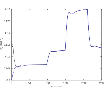
The series of simulations, as stated before intends to demonstrate the controller per-formance with different configurations. For the first simulation, figures 2.2-2.4 show respectively the velocity (manipulated variable)u(t), the outputy(t) = s(1,t)and the parameters estimates for thetunedadaptive NMPC controller of table 2.2 (whereρis the control effort or penalty weight). Take notice that the parameter estimates converge in the first 30hthereby, maintaining the controller performance. The response to a sudden change

in set-point has a settling time smaller than 12.5hand an approximately 15₋20% over-shoot. Figure 2.4 shows the estimated parameters, for initial values ˆθ1(0) =0.1, ˆθ2(0) =0.3.

The estimates converge to the nominal values given in table 2.1. The estimation gains and the convergence coefficients are given in table 2.3. Figure 2.7 shows the Lyapunov function decreasing for each step set-point change. Because the control law is well tuned the stability condition is not active during all simulation. Finally, figures 2.5 and 2.6 show, respectively substrate and biomass profiles.

(49)

2.7. APPLICATION TO A FIXED-BED TUBULAR BIOREACTOR WITH CONTOIS KINETICS

Table 2.3: Estimation and convergence parameters.

Parameters Value

kpx 0.1 IN+1

kps 0.1 IN+1

γx 0.1

γs 1.0×10−3

0 50 100 150 200 250

Time [h]

0.1 0.105 0.11 0.115 0.12 0.125 0.13

u(t) [ms