Ricardo Sérgio Gomes Almeida Loução
Bachelor of ScienceStructural Connectivity based on Diffusion
Kurtosis Imaging
Dissertation submitted in partial fulfilment of the requirements for the degree of
Master of Science in Biomedical Engineering
Adviser: Hugo Alexandre Ferreira, Auxiliary Professor,
Faculty of Sciences of University of Lisbon
Co-adviser: Rita G. Nunes, Auxiliary Investigator,
Structural Connectivity based on Diffusion Kurtosis Imaging
Copyright © Ricardo Sérgio Gomes Almeida Loução, Faculty of Sciences and Technology, NOVA University of Lisbon.
The Faculty of Sciences and Technology and the NOVA University of Lisbon have the right, perpetual and without geographical boundaries, to file and publish this dissertation through printed copies reproduced on paper or on digital form, or by any other means known or that may be invented, and to disseminate through scientific repositories and admit its copying and distribution for non-commercial, educational or research purposes, as long as credit is given to the author and editor.
A c k n o w l e d g e m e n t s
Funny that this is the first piece of text in this document, and yet was the last one to be written. . .
This was, by far, the hardest task I’ve ever set myself to do (come to think of it, I was actually told to do this, but I just wanted to add drama to the text). Writing this dissertation often drew me out of my strength and it was through the support of friends and family that I kept on going. This chapter is dedicated to them.
First and foremost, my advisor and co-advisor, Prof. Hugo Ferreira and Prof. Rita Nunes (to whom I’ve already been granted permission to address to simply as Rita -a gre-at -accomplishment!). Without them none of this w-as possible. No thesis pl-an, obviously, but more importantly, no lengthy, yet highly productive, meetings discussing the paths to take and the results obtained, while still maintaining the casual register, always making me feel at easy in their presence. To them I would like to express my greatest gratitude, not only for the time wasted with me but also for the high degree of patience displayed. Prof. Hugo, please note that I did not forget we still have a bottle of Oporto wine to finish and a tandem jump to do!
Still on an academic note, I would like to thank my overseas counsellors, Marta Cor-reia, Rafael Neto-Henriques and André Ribeiro. Each in their own field of expertise, provided me with invaluable tips and information, which without them, this dissertation would be seriously undermined.
On a more personal note, thanks are due to my faculty buddies, Ameixa, Mota, Juliana (aka Júlia), Rito, Ana Carolina (aka Fradinho), Flávio (aka Prof. Rocha), Débora (here’s your paragraph!!) and Soraia, for forcing me to laugh in times of utter despair and for forcing me to make them laugh in their time of despair, increasing the overall happiness in the world. Furthermore, I would like to thank them for all of the parties attended together, all of the nights where sorrows were drowned and hangovers that followed suit!
Carrying on with the personal thank you note, throughout my academic years I have established special connections with special people with whom I have the pleasure to share a very special bond. To Lina, Jéssica, Dalila, Idalizia, Ana Leonor, Franga and Swag (and Onofre!), thanks for all of the coffees we’ve had together, all of the smiles that
brightened my day and just everything you did for me/with me.
meus irmãos quero agradecer por todos os dias esticarem o meu limite de paciência (que me ajudou imenso [!!!] a lidar com as múltiplas personagens que fui conhecendo) e por estarem sempre dispostos a alinhar nas minhas baboseiras, por mais parvas que elas sejam, fruto de um longo dia de tese. E, finalmente, à pessoa que realmente tornou isto possível, à minha mãe. Sem a qual não teria nascido, e consequentemente não teria atingido esta grande meta da minha vida (entre muitas outras coisas, que não há espaço para dizer e por isso ficarão para outra altura). A vós este documento.
A b s t r a c t
Structural connectivity models based on Diffusion Tensor Imaging (DTI) are strongly
affected by the technique’s inability to resolve crossing fibres, either intra- or
inter-hemis-pherical connections. Several models have been proposed to address this issue, includ-ing an algorithm aiminclud-ing to resolve crossinclud-ing fibres which is based on Diffusion Kurtosis
Imaging (DKI). This technique is clinically feasible, even when multi-band acquisitions are not available, and compatible with multi-shell acquisition schemes. DKI is an
exten-sion of DTI enabling the estimation of diffusion tensor and diffusion kurtosis metrics. In
this study we compare the performance of DKI and DTI in performing structural brain connectivity.
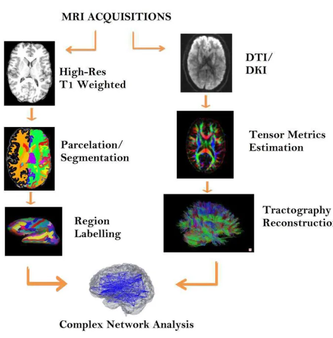
Six healthy subjects were recruited, aged between 25 and 35 (three females). The MRI experiments were performed using a 3T Siemens Trio with a 32-channel head coil. The scans included a T1-weighted sequence (1mm3), and a DWI with b-values 0, 1000 and 2000s.mm−2. For each b-value, 64 equally spaced gradient directions were sampled. For DTI fitting only images with b-value of 0 and 1000s.mm−2were considered, whereas for the DKI fitting, the whole cohort of images were considered. To fit both DTI and DKI tensors, extract the metrics and perform tract reconstructions, the toolbox DKIu was used, and the structural connectivity analysis was accomplished using the MIBCA toolbox.
Tractography results revealed, as expected, that DKI-based tractography models can resolve crossing fibres within the same voxel, which posed a limitation to the DTI-based tractography models. Structural connectivity analysis showed DKI-based networks’ abil-ity to establish both more inter-hemisphere and intra-hemisphere connections, when compared to DTI-based networks. This may be a direct consequence of the inability to resolve crossing fibres when using the DTI model. The DKI model ability to resolve crossing fibres may provide increased sensitivity to both inter- and intra-hemispherical connections.
DKI seems to provide additional insights into structural brain connectivity by resolv-ing crossresolv-ing fibres, otherwise undetected by DTI.
Keywords: Diffusion Tensor Imaging, Diffusion Kurtosis Imaging, Tractography,
Struc-tural Connectivity
R e s u m o
Modelos de conectividade estrutural baseados em Imagem por Tensor de Difusão (DTI) são fortemente afetados pela limitação da técnica em resolver cruzamentos de fibras intra-voxel, quer a um nível de ligações intra-hemisféricas ou inter-hemisféricas. Vários modelos têm sido propostos para tentar colmatar este problema, incluindo um algoritmo focado para a resolução destes cruzamentos de fibras baseado em Imagem por Curtose de Difusão (DKI). Esta técnica é clinicamente exequível, mesmo quando esquemas de aquisiçãomulti-band não estão disponíveis. DKI funciona como uma extensão do DTI, na medida em que permite estimar métricas do tensor de difusão assim como do tensor de curtose. Neste estudo comparamos o desempenho do DKI e do DTI em conectividade estrutural do cérebro.
Seis sujeitos saudáveis foram recrutados, com idades compreendidas entre os 25 e 35 anos (três de sexo feminino). As aquisições de Ressonância Magnética (IRM) foram executadas utilizando um aparelho 3T Siemens Trio com uma bobina de receção de 32 canais. As aquisições incluíram uma sequência ponderada em T1 (1mm3), e DWI com valores de b de 0, 1000 e 2000 s.mm−2. Para cada valor de b, 64 direções de gradiente igualmente espaçadas foram adquiridas. Para estimar o tensor de DTI foram apenas consideradas imagens com valor de b igual a 0 e 1000s.mm−2, mas para estimar o tensor DKI, foram utilizadas todas a imagens adquiridas. Para estimar os tensores de difusão e curtose, extrair as métricas e realizar a reconstrução por tractografia, foi utilizado o programa DKIu, e para a análise da conetividade estrutural foi utilizada a toolbox MIBCA.
Os resultados das tractografias revelaram, como esperado, que os tractos estimados com base em algoritmos de DKI conseguem resolver cruzamento de fibras dentro do mesmo voxel, que é uma limitação da abordagem por DTI. A análise da conectividade estrutural revelou resultados interessantes no que toca à capacidade das redes computa-das por DKI reonhecerem mais ligações quer inter-hemisféricas quer intra-hemisféricas, quando comparadas com as redes computadas por DTI. Isto pode ser uma consequência directa da incapacidade de resolução de cruzamento de fibras quando se utiliza o mo-delo de DTI. A resolução de fibras cruzadas pelo momo-delo DKI pode providenciar uma sensibilidade acrescida a ligações quer inter-hemisféricas quer intra-hemisféricas.
mostram agrupamentos que englobam ambos os hemisférios, com múltiplas ligações inter-hemisféricas dentro do mesmo agrupamento.
As métricas de conectividade globais e locais também foram estudadas, mas parecem sofrer de grande variabilidade, pelo que os resultados foram inconclusivos. Esta variabili-dade pode dever-se a falta de reproducibilivariabili-dade das métricas estudadas ou do número de sujeitos considerados ter sido baixo.
DKI parece fornecer nova informação para a conectividade estrutural do cérebro ao resolver cruzamento de fibras, mas a verdadeira extensão dessa melhoria ainda está em estudo.
Palavras-chave: Imagem por Tensor de Difusão, Imagem por curtose de difusão, Tracto-grafia, Conectividade Estrutural
C o n t e n t s
List of Figures xv
List of Tables xvii
Acronyms xix
1 Introduction 1
1.1 Context and Motivation . . . 1
1.2 Objectives and Dissertation Plan . . . 2
1.3 State-of-the-Art . . . 3
1.4 Dissertation outputs . . . 5
2 Theoretic Underpinnings 7 2.1 Diffusion and MRI . . . . 7
2.1.1 Physics of MRI . . . 7
2.1.2 Diffusion Weighted Imaging . . . . 9
2.1.3 Imaging Sequences . . . 9
2.2 Diffusion Tensor Imaging . . . . 11
2.2.1 DTI Formulation and Metrics . . . 11
2.2.2 DTI Advantages and Pitfalls . . . 13
2.3 Diffusion Kurtosis Imaging . . . . 14
2.3.1 DKI Formulation and Metrics . . . 14
2.3.2 DKI Advantages and Pitfalls . . . 16
2.4 Tractography . . . 16
2.4.1 DTI-based Tractography . . . 16
2.4.2 DKI-based Tractography . . . 18
2.4.3 Tractography Overall Shortcomings . . . 20
2.5 Brain Connectivity . . . 20
2.5.1 Networks: Principles and Definitions . . . 21
2.5.2 Complex Network Analysis Metrics . . . 21
2.5.3 Brain Network . . . 23
C O N T E N T S
3.1 Dataset and Acquisitions . . . 25
3.2 Image Processing Tools and Steps . . . 26
3.3 Statistical Analysis . . . 28
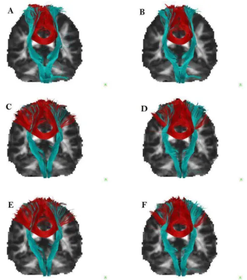
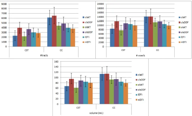
4 Results and Discussion 33 4.1 Tractography . . . 33
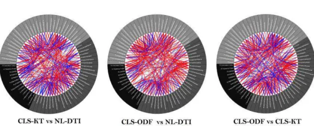
4.2 Connectivity . . . 36
4.2.1 Global Connectivity . . . 36
4.2.2 Local Connectivity . . . 38
5 Conclusions and Future Work 45
Bibliography 49
A Appendix 1 - ROI List 55
B Appendix 2 - Tractography results 57
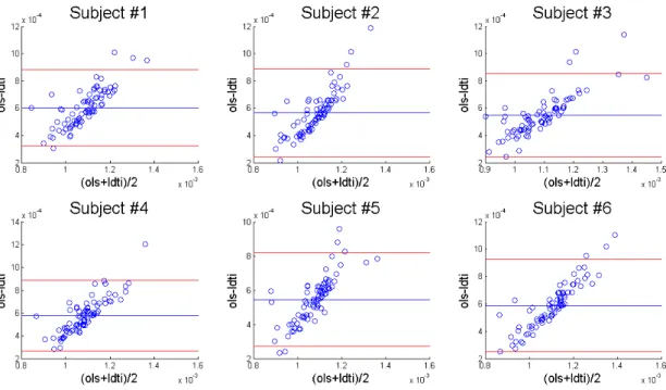
C Appendix 3 - Bland Altman Plots 65
L i s t o f F i g u r e s
2.1 T1 and T2 relaxation times [35] . . . 8
2.2 PGSE sequence scheme. Adapted from [39]. . . 10
2.3 SS-EPI scheme [35]. . . 11
2.4 Diffusion tensor in different constriction media [43] . . . . 12
2.5 Fibre reconstruction from the main diffusion direction map. . . . 17
2.6 3D geometry of DKI-ODF and DTI-ODF. Adapted from [54] . . . 18
2.7 3D geometry of DT, KT and ODF [51] . . . 19
2.8 Noncommutative properties of tractography algorithms [53]. . . 20
2.9 Graph metrics[58] . . . 22
2.10 Three types of network configuration[60] . . . 23
2.11 Diagram showing the relationships between all types of networks [58]. . . . 24
3.1 Generic placement of the ROI’s for tract isolation based on [67]. . . 28
3.2 Processing steps diagram . . . 29
4.1 Tractography reconstructions for Subject 1 . . . 34
4.2 Bar plots of the streamline statistics . . . 35
4.3 Misinterpreted DTI tracts . . . 35
4.4 DKI and DTI based structural connectivity connectograms . . . 36
4.5 Difference connectograms . . . . 37
4.6 Modularity connectograms with metrics rings . . . 39
4.7 Bland-Altman plots of AD from CLS-KT and NL-DT . . . 41
B.1 Tractography reconstructions for subject 1 . . . 58
B.2 Tractography reconstructions for subject 2 . . . 59
B.3 Tractography reconstructions for subject 3 . . . 60
B.4 Tractography reconstructions for subject 4 . . . 61
B.5 Tractography reconstructions for subject 5 . . . 62
B.6 Tractography reconstructions for subject 6 . . . 63
C.1 Bland-Altman plots of AD from CLS-KT and NL-DT . . . 66
C.2 Bland-Altman plots of RD from CLS-KT and NL-DT . . . 66
L i s t o f F i g u r e s
C.4 Bland-Altman plots for AD from CLS-KT and L-DT . . . 67
C.5 Bland-Altman plots for RD from CLS-KT and L-DT . . . 68
C.6 Bland-Altman plots for MD from CLS-KT and L-DT . . . 68
C.7 Bland-Altman plots for AD from OLS-KT and NL-DT . . . 69
C.8 Bland-Altman plots for RD from OLS-KT and NL-DT . . . 69
C.9 Bland-Altman plots for MD from OLS-KT and NL-DT . . . 70
C.10 Bland-Altman plots for AD from OLS-KT and L-DT . . . 70
C.11 Bland-Altman plots for RD from OLS-KT and L-DT . . . 71
C.12 Bland-Altman plots for MD from OLS-KT and L-DT . . . 71
L i s t o f Ta b l e s
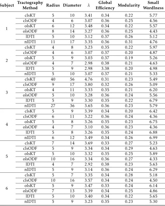
4.1 Global connectivity metrics results . . . 40 4.2 Systematically "flagged" ROI’s and respective connectivity metrics(1) . . . . 42 4.3 Systematically "flagged" ROI’s and respective connectivity metrics(2) . . . . 43
A c r o n y m s
AD Axial Diffusivity.
ADC Apparent Diffusion Coefficient.
AK Axial Kurtosis.
aMRI anatomical MRI.
BCT Brain Connectivity Toolbox.
BET Brain Extraction Tool.
CC Corpus Callosum.
CLS Constrained Least Square.
CLS-KT Constrained Least Squares fitted Kurtosis Tensor.
CST Cortico-Spinal Tracts.
DKI Diffusion Kurtosis Imaging.
dODF diffusion Orientation Distribution Function.
dPDF diffusion displacement Probability Density Function.
DSI Diffusion Spectrum Imaging.
DT Diffusion Tensor.
DTI Diffusion Tensor Imaging.
DWI Diffusion Weighted Imaging.
FA Fractional Anisotropy.
FAK Kurtosis Fractional Anisotropy.
FID Free Induction Decay.
AC R O N Y M S
HARDI High Angular Resolution Diffusion Imaging.
IC Internal Capsule.
KT Kurtosis Tensor.
L-DT Linearly fitted Diffusion Tensor.
MD Mean Diffusivity.
MDD Main Diffusivity Direction.
MIBCA Multimodal Imaging Brain Complexity Analysis.
MK Mean Kurtosis.
MRI Magnetic Resonance Imaging.
nL-DT Non-Linearly fitted Diffusion Tensor.
OLS Ordinary Least Square.
OLS-KT Ordinary Least Squares fitted Kurtosis Tensor.
PGSE Pulsed Gradient Spin Echo.
RD Radial Diffusivity.
RF Radio Frequency.
RK Radial Kurtosis.
ROI Region of Interest.
SPM Statistical Parametric Mapping.
SS-EPI Single Shot Echo Planar Imaging.
TRSE Twice Refocused Spin Echo.
uDKI United Diffusion Kurtosis Imaging.
WM White Matter.
C
h
a
p
t
e
r
1
I n t r o d u c t i o n
1.1 Context and Motivation
Diffusion Weighted Imaging (DWI), a kind of Magnetic Resonance Imaging (MRI)
sensi-tive to diffusion, has been continuously evolving since its introduction, in the mid-1980’s,
proving its worth against the other techniques used to inspect the human body in a non-invasive way. Based on the principle of diffusion observed in water molecules, DWI has
been particularly relevant in the study of regions where diffusion motion tends to be
anisotropic. This is the case of white matter fibres in the brain. Such behaviour helps to understand the organization and connections of the structures in soft tissues at a
macro-scale. Hence, the study of the whole brain’s structural connectivity can be performed using the information provided by DWI techniques.
In its early days, DWI were modelled describing water diffusion as a scalar, in order
to assess whether the diffusion was higher (brighter voxels) or lower (darker voxels) in
a particular region. But this description was found to be very limited and there was the need to characterize and not only quantify diffusion but also its three-dimensional
orientation. Diffusion Tensor Imaging (DTI) was then introduced. In its foundation lies
the assumption that water diffusion can be approximated by a Gaussian model, and that
a full characterization of the water diffusion can be accomplished estimating a diffusion
tensor. This lead to a revolution in the imaging world, allowing the firstin vivo visualiza-tion of brain fibres, through means of tractography, and numerous breakthroughs in the perception of structural modifications due to pathological conditions.
C H A P T E R 1 . I N T R O D U C T I O N
in two distinct directions, crossing each other. Using the DTI model, voxels with multiple fibres are assigned lower fractional anisotropy (anisotropy intrinsic to each voxel) than the real one, due to the contributions of multiple fibres, lowering the overall anisotropy for that voxel. In addition to that, the overall Main Diffusivity Direction (MDD) for
that voxel is also affected. This introduces both false positives and false negatives tract
connections in DTI-based tractography reconstruction. Furthermore, the Gaussian model seems to be a poor fit to the biological diffusion scenario. The high complexity of the
structures at hand (myelin sheaths, cellular organelles, etc.) have been shown to result in water molecular diffusion to look more like a sharper and thinner version of the Gaussian
distribution. Thus, using a Gaussian model to characterize diffusion in biological tissues
is often inaccurate.
To help mitigate these limitations, a new set of techniques have been developed, such as Diffusion Spectrum Imaging (DSI) and High Angular Resolution Diffusion Imaging
(HARDI). These techniques offered improvements on the DTI flaws, particularly in
solv-ing the tractography-related limitations, acquirsolv-ing images with multiple shells. These multi-shell acquisition schemes enable the description of the full diffusion function
us-ing measurements such as displacement, zero-probability and kurtosis. But this extra sensitivity comes with a hefty cost: lengthy acquisition times. This completely rules out the implementation of these techniques in a clinical environment.
Diffusion Kurtosis Imaging (DKI) was also developed to deal with the limitations of
DTI. Working with a lower range of b-values than the previous techniques, DKI is both clinically feasible and allows for multi-shell acquisition schemes. DKI also abandons the Gaussian model, extending it to include a kurtosis dependent term, which is a statistical measurement that determines the degree of deviation of a distribution from a Gaussian distribution. In addition to estimating all DTI-derived metrics, DKI modelling also allows estimating kurtosis derived metrics, which can better characterize the spatial architecture of tissue microstructure. Therefore, the DKI model acts as an extension of the DTI model.
These improved methods lead to the growing interest in studying the brain’s connec-tivity in vivoand non-invasively. Tractography reconstructions produce large datasets of anatomical connections patterns, and to better analyse these patterns, they are often represented as complex networks. Brain networks comprise nodes (vertices) and links (edges), and the network’s inherent metrics can be very useful to understand the struc-tural organization of the brain, both locally and as a whole.
Therefore, improvements in imaging techniques may reveal important pieces of in-formation otherwise omitted. Inin-formation like this may lead to a more accurate recon-struction of the brain fibres, making the end result a more robust tractography, and, consequently, a better characterization of the brain’s structural connectivity.
1.2 Objectives and Dissertation Plan
This dissertation has two primary objectives:
1 . 3 . S TAT E - O F -T H E -A R T
• Compare the performances of DTI and DKI-based tractographies, particularly in resolving intra-voxel crossing fibres.
• Compare network metrics, both local and global, characterizing DTI and DKI net-works.
To do so, the present dissertation has been structured so as to first cover the current state-of-the-art concerning structural connectivity and DKI. Afterwards, the reader will be given a comprehensive explanation of the relevant theoretic underpinnings of diffusion
MRI, such as acquisition schemes and formulations; tractography, what is it and how is it performed; and connectivity, from networks to biological inferences. Secondly, the reader will be introduced to the methods and materials used to perform this study, datasets used, image processing steps and statistical analysis. Thirdly, the results will be presented to the reader, according to each study, as well as their discussion. Finally, the conclusion and future work chapter will summarize the dissertation’s findings and inform the reader on potential paths to take in future endeavours.
1.3 State-of-the-Art
The brain has been a subject of study ever since there was a need to understand how it worked. Primal research methods were performed ex-vivo, during autopsies, since there was no other way to inspect the human brain without compromising its integrity. Later, with the development of imaging technologies, research evolved into thein vivomethods we have today, such as MRI [1]. White matter has been focus of study many times [2, 3, 4, 5], particularly because it plays a key role in the brain’s structure and function.
Through the modification of MRI acquisition schemes, it is possible to sensitize MRI to the random motion of water, or diffusion. Since water diffusion is bounded by cellular
structures, which in the brain’s case are myelin sheaths, it is possible to relate the water diffusion to the microstructures that limit it. The development of diffusion sensitive MRI
techniques brought upon an increase in the brain structure studies, which are based on fibre tract reconstruction, or tractography [6, 7, 8, 9, 10, 11]. Tractography reconstruction is based on the grounds that water diffusion in the brain is conditioned by axons and
their myelin sheats, and thus the water molecules show a preferred direction of diffusion
(along the fibres rather than across). This is then used to assess inter-voxel connectivity based on the preferred direction of diffusion. All of this makes diffusion weighted MRI
a prime tool to assess, in a non-invasive way, the direction of fibres in white matter and, consequently, brain connectivity.
DTI was the first technique to be used to extract information on the characterization of the white matter fibres for fibre tracking [6, 7]. A diffusion tensor was fitted to the
diffusion distribution assuming that the displacement function of the molecules in the
C H A P T E R 1 . I N T R O D U C T I O N
neuroradiology [13]. But it showed several limitations, like diffusion not being Gaussian
in biological tissues and lack of sensitivity to crossing fibres inside the same voxel [14, 15]. To mitigate these limitations, two approaches were used: whether to use different
imag-ing models, from model free approaches like Q-Ball Imagimag-ing [16], Diffusion Spectrum
Imaging [17] or Hybrid Diffusion Imaging [18], to modelled approaches like DKI [19]; or
to use new and refined tractography algorithms, such as Spherical Deconvolution [20] or High Angular Resolution Diffusion Imaging [8], and also expanding on the deterministic
(conventional) tractography to probabilistic [21] and global [22] algorithms.
Studies have been carried out comparing the performance of the tractography algo-rithms, on synthetic cases [23] and on real data [24], and global tractography seems to provide with better results, followed by probabilistic and then by deterministic. In the deterministic algorithms, single compartmental models (like DTI) are out-performed by any other of the above mentioned, due to the lack of sensitivity to the crossing fibres. Despite their optimistic results, both global and probabilistic tractography algorithms are computationally very time consuming [25], which rules them out for uses outside research, at least until computational advances are reached to meet the clinical time de-mands. Deterministic tractography computation times are shorter and therefore offer a
better trade offbetween results and computation time. As for the the model free diffusion
models, all of these techniques show better results with multiple and high b-values [16, 26], resulting in lengthy acquisition schemes. In turn, this also becomes a big limitation to their use in the clinical scope.
The recent introduction of DKI has provided the medical and scientific community with more tools to evaluate axonal and myelin integrity in white matter regions [19], at clinically feasible times while maintaining the multi-shell acquisitions (multiple b-values). In fact, recent studies reveal that DKI information can be of more value than that of DTI, either from a microstructural point of view [27, 28, 29] or from a connectivity stand point [30, 31]. It was further introduced by Rudrapatna et. al [32] the notion that DKI could present both complementary and exclusive information, proposing that DKI not only provides unique information but increased sensibility to the microsctructures of white matter. DKI then proves itself to be an advantageous method for studying the structural organization and connectivity of healthy white matter [33], and to assess structural modifications linked to pathological cases [34]. Furthermore, DKI is able to successfully address the crossing fibres problem, brought upon by the DTI model. This increased sensitivity may yield additional insights when it comes to whole brain connectivity.
Studies encompassing both DKI and connectivity are yet few in numbers, with only a few studies assessing human brain asymmetric connectivity based on DKI [30], with stud-ies of whole brain connectivity still non-existent. It is therefore important to fill in this gap in the research, and determine whether or not DKI-based whole brain connectivity yields any assets beyond those of DTI-based connectivity.
1 . 4 . D I S S E R TAT I O N O U T P U T S
1.4 Dissertation outputs
Throughout the development of this dissertation, several pieces of work were performed, either part of the main project or as side-projects, that produced some type of output. As part of the main project, the following works have resulted:
Publications
• Loução, R.; Nunes, R.G.; Neto-Henriques, R.; Correia, M. M.; Ferreira, H. A., "Human brain tractography: A DTI vs DKI comparison analysis", 2015 IEEE 4th Portuguese Meeting on Bioengineering (ENBENG) proceedings, pp.43-44, 26-28 Feb. 2015
Communications
• Loucao, R.; Nunes, R.G.; Neto-Henriques, R.; Correia, M.; Santos-Ribeiro, A., Ferreira, H.A., “Structural Connectivity Based on Diffusion Kurtosis Imaging”
accepted to ESMRMB, 1-3 October 2015, Edinburgh, Scotland
• R. Loução, R. G. Nunes, R. Neto-Henriques, M. M. Correia, H. A. Fer-reira, “Human brain tractography: a DTI vs DKI comparison analysis”, 4th Portuguese BioEngineering Meeting, 26-28 February 2015, Porto, Portugal.
• A. Santos-Ribeiro, L. M. Lacerda, R. Neto-henriques, R. Maximiano, R. Loução, D. Nutt, J. McGonigle, H. A. Ferreira, "MIBCA, A toolbox for pro-cessing and analysis of multimodal imaging and connectivity data", 2015 In-ternational Conference on Brain Informatics & Health, 30 Aug - 2 Sept 2015, London, UK
As a side-project, a 3D tractography visualizer was developed in Unity. The final result will incorporate the Unity environment, the Leap Motion and Oculus Rift, to make an immersive 3D visualizer of tractography, controlled solely by the Leap Motion sensor. Another side-project was the study of the effect of downsampling the amount of b-vectors
towards the minimum amount required to estimate the kurtosis tensor (see 2.3.1), as part of an ERASMUS internship project. From this project, it was determined that only kurtosis tensor related metrics (see 2.3.1) are affected by the downsampling, whereas the
diffusion tensor based metrics (see 2.2.1) remained unchanged. These projects were not
C
h
a
p
t
e
r
2
T h e o r e t i c U n d e r p i n n i n g s
In this chapter, the reader will be introduced to all of the theoretic concepts needed to understand the content of the remaining chapters of this dissertation. First, an overview on MRI and how it can be sensitized to water diffusion in biological tissues. Then, more in
depth, the two methods of DWI used in this work will be explained, DTI and DKI, from their formulation to advantages and pitfalls. Moving on, the tractography section will inform the reader on how these reconstructions are performed, based on the diffusion
and kurtosis tensors. Finally, an overview on connectivity will be presented, describing what it is and why it is used in this context, while also introducing connectivity metrics and their biological interpretation.
2.1 Di
ff
usion and MRI
2.1.1 Physics of MRI
MRI is a non-invasive diagnosis technique used to provide anatomical images of the human body, usually with a high spatial resolution and soft tissue contrast. To do so, MRI focuses on the atomic nuclei magnetic properties, in particular, those of the hydrogen nucleus. A hydrogen nucleus is composed by a proton which precesses around itself, described by the angular momentum of the nucleus, called spin. Other nuclei could be considered, but the hydrogen nucleus is the preferred one due to its abundance in water and fat, two main elements of the human body.
C H A P T E R 2 . T H E O R E T I C U N D E R P I N N I N G S
occupy inside the magnetic field. Since one level has a slightly lower energy than the other, the lower energy level will have more protons than the higher energy level; this difference
causes the net magnetization to be different from zero. To this magnetic component we
call longitudinal magnetization (M0).
The frequency at which protons precess when immersed in the magnetic field is given by
ω0=γB0 (2.1)
whereω0is the Larmor frequency,γ is the gyromagnetic ratio of the atom andB0is the intensity of the magnetic field. In order to acquire signal, a disruption has to be made in the system. So, Radio Frequency (RF) pulses are applied in a direction perpendicular to that ofB0, creating a new magnetic component called transverse magnetization (Mxy). The RF pulse must be applied at the Larmor frequency so as to induce resonance. This forces the spins to precess at a given angle from the original magnetic field on the xy plane (provided we consider z as the axis longitudinal to B0), and this angle depends on the pulse’s characteristics (duration and intensity). Finally, when the RF pulse is switched off, the spins relax into the main direction again. Since these processes take time to occur,
and the time taken is intrinsic to each tissue, it is possible to establish a correspondence between tissue type and the signal acquired. There are two different relaxation times
to be considered. T1, or spin-lattice relaxation time, is the time taken for 63% ofM0to recover after a 90°RF pulse. T2, or spin-spin relaxation time, corresponds to the time it takes for 37% ofMxyto be obtained due to relaxation of transverse magnetization, from a given value, determined by the RF pulse duration and intensity (see Figure 2.1). T2 is influenced also by interactions between spins, and if the inherent field inhomogeneities
Figure 2.1: T1 and T2 relaxation times [35]. Although they happen at the same time, T2 is much smaller than T1.
2 . 1 . D I F F U S I O N A N D M R I
are also considered, the relaxation will occur at a rate of T2* instead, which is shorter than T2.
The variation ofMxy is then detected by a receiving coil, in which, by induction, an electric current is generated. The decay of this current is exponential with the relaxation. The signal obtained in the coil is called Free Induction Decay (FID).
2.1.2 Diffusion Weighted Imaging
Diffusion, or brownian motion, is the random displacement of particles in a fluid. This
displacent can be characterized by the diffusion constant. At a constant temperature, the
diffusion constant D is given by Einstein’s equation [36]
D= R 2
6t (2.2)
where R2 is the mean square displacement of the particles and t the time interval during which the displacement occurred.
In an unbounded environment, the water diffusion is the same in all directions in a
given amount of time. This kind of diffusion is called isotropic diffusion. However, the
same does not apply in the human body. Due to the presence of cell membranes and other cellular structures, water molecules are conditioned in their diffusion. This means that
water molecules are allowed to travel longer distances in some directions that in others, for the same time interval. This phenomenon is called anisotropic diffusion.
In the brain’s White Matter (WM), the water in the axons is restricted by the myelin sheath and cell membrane, constituting barriers to free diffusion. This, in turn, means
that the diffusion will be more prominent along the direction parallel to the axis of the
axons. This assumption is particularly important when studying the WM microstructure.
DWI is an imaging technique that is sensitive to water diffusion. When it first
ap-peared, diffusion was modelled using a simple scalar, coded by pixel brightness. Then,
with the appearance of DTI, a full three dimensional characterization became possible. In either case, diffusion is measured through the Apparent Diffusion Coefficient (ADC). The
termapparentis used inin vivoacquisitions because it is impossible to differentiate
dif-fusion from other sources of water mobility. ADC values depend on the motion-probing gradients and on their time interval. It takes any value from 0, if no motion is present, to the diffusion coefficient D, if diffusion is the only water motion phenomenon present
[37].
2.1.3 Imaging Sequences
C H A P T E R 2 . T H E O R E T I C U N D E R P I N N I N G S
Figure 2.2: PGSE sequence scheme. Adapted from [39].
2.1.3.1 Pulsed Gradient Spin Echo
One of the most used acquisition schemes is called Pulsed Gradient Spin Echo (PGSE). Created by Stejskal and Tanner, it consists of two RF pulses, one of 90º and the second of 180º, and two magnetic gradients, with intensity G and time spanδ, before and after the 180º RF pulse[38], as seen in 2.2.
The first gradient offsets the phase of the water protons’ spins by a certain angle, and
the second one resets the phase by the same angle. However, between the application of these gradients, spins randomly lose coherence due to diffusion. This means that the
final phase of the spin will not be the same, resulting in an attenuation of the signal. This difference is the result of water diffusion, measured as the ADC.
Since diffusion in MRI acquisitions is represented as a signal decay, quantifying diff
u-sion can be achieved using a scalar D and the signal obtained can be described by:
S(b) =S0−bD (2.3)
where D is the diffusion coefficient, S0is the signal intensity with no diffusion weighting
and theb-value, defined by:
b=γ2.G2.δ2.(∆−δ
3) (2.4)
characterizes the parameters of the diffusion gradients in the acquisition sequence,
such as duration (δ), time elapsed between the onset (∆) and intensity of the gradients (G).
Manipulating these will allow different weightings of diffusion in the acquired image. A
standard value of b, for the brain, is 1000s.mm−2.
2.1.3.2 Single Shot Echo Planar Imaging
The Single Shot Echo Planar Imaging (SS-EPI) sequence is the most used sequence in diffusion weighted acquisition. This is due to its imperviousness to motion related
arte-facts and substantially low acquisition times, when compared to other sequences. During acquisition, subjects are prone to move, and this movement, during the diffusion
weight-ing gradients application, adds a phase component to the MRI signal. This component,
2 . 2 . D I F F U S I O N T E N S O R I M AG I N G
Figure 2.3: SS-EPI sequence scheme [35].
whether from head motion or from blood flow, introduces artefacts in the image that can corrupt the consistency of the acquisition if not dealt with before hand[35]. This sequence only has one RF pulse, of 180º, as seen in Fig. 2.3. Before and after the RF pulse, like PGSE, two diffusion weighting gradients are applied, but after that, a series of gradients
are also applied in order to generate several gradient echos. These extra gradients are of interchangeable polarity and are responsible for the k space line coding. By manipulating these gradients’ intensity it is possible to reduce the TE and obtain the desired diffusion
weighting [35].
2.2 Di
ff
usion Tensor Imaging
2.2.1 DTI Formulation and Metrics
In the previous sections, diffusion has been described only as a scalar. Although, for the
sake of characterizing diffusion in three dimensions and its respective anisotropy, a tensor
is needed. DTI was introduced to deal with this limitation [40]. The diffusion-weighted
signal S and the non-weighted signal S0are related according to:
lnS S0 =− 3 X i=1 3 X j=1
bijDij (2.5)
where bij is the b-matrix andDij the Diffusion Tensor (DT). The b-matrix effectively replaces theb-valuein the previous formulation, and is calculated based on the diffusion
gradients in the acquisition sequence [41], orb-vectors. The diffusion tensor comes in the
following form: d=
Dxx Dxy Dxz
Dyx Dyy Dyz
Dzx Dzy Dzz
C H A P T E R 2 . T H E O R E T I C U N D E R P I N N I N G S
In DTI, non-collinear gradient directions are applied and each gradient direction accounts for water diffusion along that direction. The estimation of the DT is increasingly precise
with the increasing of the amount of gradient directions, but the acquisition time also increases with the increase of gradient directions. The minimum amount of directions required to estimateDij, is, at least, 6 different non-collinear gradient directions, along with the non-weighted acquisition.
For the purpose of this dissertation, two fitting methods were used to estimate the DT, a linear regression method and a non-linear regression method. Both methods aim at minimizing the sum of squared differences error, but the first method uses a linear
regression whereas the second one uses a non-linear approach, which may provide with more favourable results [42].
To better understand the DT, it is often helpful to think about its shape, i.e. , that of an ellipsoid. In an isotropic scenario, the tensor assumes a spherical shape, for Dxx=Dyy=Dzz=D. On the contrary, if diffusion is anisotropic, the tensor is an elongated ellipsoid along the direction of greater diffusion, as seen in Figure 2.4. The main axis
represents the MDD, the eccentricity relates to the degree of anisotropy and its symmetry and the length shows the distance travelled as a result of diffusion.
Once the diffusion tensor is calculated, it is possible to estimate rotationally invariant
Figure 2.4: Diffusion tensor in different constriction media [43]. For unrestricted isotropic
diffusion, the water molecules move freely, and the diffusion tensor has only one
compo-nent in each axis. For restricted isotropic diffusion, the lack of fixed barriers only limits
the distance travelled and not its direction, which makes the diffusion tensor have only
one component in each axis, although smaller than that of unrestricted diffusion. For
anisotropic restricted diffusion, the molecules are restricted to a determined direction,
resulting in a diffusion tensor that has three components on each axis.
2 . 2 . D I F F U S I O N T E N S O R I M AG I N G
parameters, i.e. independent of the reference frame, like Mean Diffusivity (MD),
Frac-tional Anisotropy (FA), Axial Diffusivity (AD) and Radial Diffusivity (RD). This
indepen-dence is derived from the fact that these indices are calculated based on the eigenvalues of the diffusion tensor. The eigenvalues provide a framework that is specific to each
voxel, which means it is independent of other reference frames, like the reference frame of the scanner. The invariant measurements yield important information used to infer on the microstructures present in each voxel, and also in fibre tracking. MD represents the mean of the diffusion among all three directions, so it is determined using the following
equation:
MD=T r(D) 3 =
Dxx+Dyy+Dzz
3 (2.7)
where Tr(D) is the trace for the diffusion tensor. FA is a measurement of the anisotropy
inherent to each voxel [44]. It can range between 0, which means the diffusion is isotropic,
and 1, which means that the diffusion happens in one direction only. Consequently,
tissues with microstructures which force diffusion to have anisotropic properties will
be associated with FA values closer to 1, such as the white matter in the brain, while tissues such as grey matter, tend to display near isotropic diffusion, e.g. associated with
low values of FA. To calculate the FA, the eigenvaluesλ for each axis of the diffusion
tensor must be calculated first. By convention, the first eigenvalue λ1 gives the AD, which reflects the magnitude of diffusion along the principal component of the diffusion
ellipsoid. The eigenvaluesλ2andλ3are used to calculate the RD, i.e. the diffusion along the other two components of the diffusion ellipsoid, with
λ⊥=
λ2+λ3
2 (2.8)
The FA then comes as
FA= q
3[(λ1−(λ))2+ (λ2−(λ))2+ (λ3−λ))2] q
2(λ21+λ22+λ23)
(2.9)
whereλis the mean value of the eigenvalues
λ=1 3
3 X
i=1
λi (2.10)
2.2.2 DTI Advantages and Pitfalls
By characterizing the direction of diffusion, DTI has an unique advantage in clinical
applications, when compared to other diffusion MRI techniques. Analysis of white matter
pathology, like ischemia, axonal damage and myelination, tumor characterization and surgical planning are a few of its clinical applications.
C H A P T E R 2 . T H E O R E T I C U N D E R P I N N I N G S
The fitting to the data acquired is accomplished assuming that the random displace-ment of the water molecules follows a Gaussian model [45]. This means that the water molecules displacement distribution function can be described by a Gaussian curve. But in the human brain context this cannot be applicable. Such fitting proves to be poor, due to the high degree of complexity of the microstructures present, which makes diffusion
often behave differently from the Gaussian model[46]. Furthermore, in crossing fibres
sections, the simple Gaussian model is also not applicable, as it assumes that only one fibre population exists per voxel. In these regions, the fractional anisotropy seems to be lower, due to the contribution of two or more fibres in different directions and the MDD
cannot be attributed correctly. In further applications like Tractography (see 2.4), a poor characterization of MDD can result in a reconstruction of false positive or false negative tracts, which in turn introduces anatomical inaccuracies in the tractography.
2.3 Di
ff
usion Kurtosis Imaging
As stated before, DTI is based on Gaussian model fitting, yet this fitting yields non-optimal results for biological tissues with highly complex microstructures. DKI is a method that replaces the Gaussian model by a kurtosis based model. Kurtosis is a statisti-cal measurement that determines the deviation of a distribution in relation to a Gaussian distribution, measured by a parameter K. If K>0, the distribution is more concentrated around the mean value; if K=0 the distribution is Gaussian; if K<0 the tails of the distri-bution are wider and its peak lower, compared to those of a Gaussian. Although K can be positive or negative, in biological tissues, K has been shown to have only positive values [47].
DKI is compatible with multi-shell acquisitions, i.e. multiple b-values. This means that the acquisition times are increased when compared to those of DTI. A DTI sequence may take 3-6 mins [48] and a DKI sequence takes about 10 mins [49]. This makes DKI a feasible technique in the clinical scope, which can ease the transition from DTI to DKI from a clinical stand point, and ultimately replace DTI as the main DWI technique in the clinical context.
2.3.1 DKI Formulation and Metrics
The Kurtosis Tensor (KT), unlike DT, is a 3x3x3x3 matrix. This allows for an improved characterization of the non-Gaussian diffusion in space. To estimate such a tensor, at
least 15 non-collinear diffusion gradients must be applied, beyond the 6 required for the
DT, with no less than threeb-values. Just like for the DT, two fitting methods were used to estimate the KT. The first one was Ordinary Least Square (OLS) and the second one was Constrained Least Square (CLS). The OLS method is a standard method which finds the optimal solution that minimizes the sum of squared differences error. But OLS can
provide implausible estimates for the KT in biological tissues. So, to account for this
2 . 3 . D I F F U S I O N K U R T O S I S I M AG I N G
limitation of OLS, CLS uses constrains in the estimates to ensure that the tensor assumes plausible biological values.
The signal acquired by the receive coils is quantified using
lnS S0
=−bDapp+ 1 6b
2D2
appKapp (2.11)
whereDappandKapp are the apparent diffusion and kurtosis. These relate to the diffusion and kurtosis tensors,Dij andWijkl respectively, in the following way:
Dapp=
3 X i=1 3 X j=1
ninjDij (2.12)
Kapp=
MD2 Dapp2
3 X i=1 3 X j=1 3 X k=1 3 X l=1
ninjnknlWijkl (2.13)
werenis the unit vector that describes the direction of the diffusion gradient.
Analogously to DT, KT also has some important rotationally invariant measurements associated to them: Mean Kurtosis (MK), Axial Kurtosis (AK), Radial Kurtosis (RK) and Kurtosis Fractional Anisotropy (FAK)[47]. MK, as MD, provides a measure of the overall kurtosis, estimated as the average of directional kurtosis, defined by:
MK= 1
N
3 X
i=1
(Kapp)i (2.14)
To calculate the FAK, first it is necessary to rotate the kurtosis tensor W from the Cartesian coordinate system to the coordinate system defined by the eigenvectors of D ([50])
b
Wijkl=
3 X i=1 3 X j=1 3 X k=1 3 X l=1
ei′iej′iek′iel′iWi′j′k′l′ (2.15)
where eij are the elements of the 3D rotation matrix defined by the eigenvectors and b
Wijkl the elements of the rotated kurtosis tensor. Once Wbijkl is computed, the values of the kurtosis tensor on the diffusion ellipsoid three main axes, with i=1, 2 and 3, are
determined by
κi=
MD2
λ2i .Wbiiii (2.16)
resulting in AK being
κk=κ1 (2.17)
and RK
κ⊥=
κ2+κ3
2 (2.18)
similarly to the DTI analogous measurements. Finally, FAK comes as
FAk= p
3[(κ1−(κ))2+ (κ2−(κ))2+ (κ3−(κ))2] q
2(κ21+κ22+κ23)
C H A P T E R 2 . T H E O R E T I C U N D E R P I N N I N G S
whereκis the mean value of the kurtosis over the diffusion ellipsoid
κ=1 3
3 X
i=1
κi (2.20)
FAK is close to one when there is a value ofκi substantially larger than the other two, and close to zero when all three values ofκare similar to each other.
2.3.2 DKI Advantages and Pitfalls
The DKI model has similar applications in the clinical scope to those of DTI. Additionally, it can provide with more detailed information about tissue microstructure, and even perform biological modelling of diffusion [51]. As opposed to DTI, DKI can account for
multiple fibre populations in the same voxel, which may result in more anatomically accurate tractography.
This model also has its own pitfalls. For being a fairly recent technique it is still not very established. For that reason, it isn’t often used in the clinical scope, it is still considered only as a research tool. Furthermore, the longer acquisition times and more stringent hardware requirements, due to high gradient strength for example, can be a deterrent from using this technique.
2.4 Tractography
One of the primary applications of the information on the direction of diffusion is fibre
tract reconstruction, or tractography. The main purpose of tractography is to determine intervoxel connectivity based on the anisotropic diffusion of water [6]. In this section we
will cover the tractography algorithms performed, for both DTI and DKI-based tractogra-phies.
2.4.1 DTI-based Tractography
DTI Fibre tracking is based on the assumption that a tract can be represented as a curve in space[7], using the Frenet equation:
dr(s)
ds =t(s) (2.21)
were r(s) is a vector, parameterized by the arc-length, s, of the trajectory, and t(s) is the unit tangent vector to r(s) at location s.
Since there is no way of calculating the tangent vector through analytical processes, numerical methods, like Euler integration and Runger-Kutta methods, were first used [7]. DTI-based tractography algorithms have since evolved and can now be divided into 3 classes:
2 . 4 . T R AC T O G R A P H Y
Figure 2.5: Fibre reconstruction from the main diffusion direction map. The blue line
indicates the path that a tract follows during reconstruction, and the lines represent the main diffusivity direction for each voxel.
1. Deterministic, characterized by the assumption that the principal eigenvector is parallel to the dominant direction of the fibre, with integration of neighbouring pixels to define smooth trajectories [40]. The tangent vector is then determined by the eigenvectorǫ1associated with the largest eigenvalue,λ1of the diffusion tensor, using the following relationship:
t(s) =ǫ1(r(s)) (2.22)
Combining the equations 2.21 and 2.22, we obtain
dr(s)
ds =ǫ1(r(s)) (2.23) which can be solved forcing the initial condition for each tract to be
r(0) =r0 (2.24)
where r0 is the starting point for a given tract. This translates into an iterative method of fibre tracking, starting in one point and recursively following the diff
u-sion "path" through the main diffusivity direction for each voxel, given by the DT
greater eigenvalue. Figure 2.5 shows the the reconstruction based on the principal eigenvector.
2. Probabilistic, in which the most favourable path between predetermined regions is evaluated. To do this, probabilistic maps of fibre connectivity for the whole brain are computed. This approach is different from the deterministic because the
tracking is computed along a continuous line, instead of a discrete vector [9];
3. Global, which estimates the local fibre orientations and then propagates them throughout the voxels to obtain estimates of connections between several brain locations, using a Bayesian propagation model [52].
However, they all share common grounds as to how to generate a tract [53]:
• reconstruction is terminated if the streamline enters a region where the FA is be-low a predetermined threshold. This condition is imposed so that the fibre recon-struction does not occur in regions where diffusion is not anisotropic, such as grey
C H A P T E R 2 . T H E O R E T I C U N D E R P I N N I N G S
• reconstruction is terminated if the maximum angle that is taken between voxels is above a predetermined threshold. This condition avoids the reconstruction of spurious tracts as a result of sudden changes in direction from one voxel to another.
Only deterministic algorithms were performed throughout this study, but the other algorithm categories were presented to give the reader the full scope.
DTI-based tractography, as seen before, has a significant pitfall, which is the fact that it cannot reliably predict fibre population directions for voxels with two or more intersecting populations. So there is a need to introduce models that can deal with this problem, often called "fibre crossing problem" [15, 55, 56].
2.4.2 DKI-based Tractography
DKI-based tractography is yet to be fully optimized, with only two methods created thus far. Both methods were incorporated in this dissertation and later on compared for performance.
2.4.2.1 Orientation Distribution Function based Tractrography
The first method to reconstruct fibres from DKI was based on the diffusion Orientation
Distribution Function (dODF), proposed by Lazar et al. in 2008 [54], and later on opti-mized [57]. dODF is a function that characterizes the spacial orientation of a distribution, in this case water diffusion, and is defined by:
Figure 2.6: 3D geometry of DKI-ODF (left) and DTI-ODF (right). The DKI-ODF is able to account for the fibre crossings, for two fibres (top left) and three (bottom left), whereas DTI-ODF shows a geometry similar to that of isotropic diffusion. Adapted from [54].
2 . 4 . T R AC T O G R A P H Y
Ψ
α( ˆn) =
1
Z
Z ∞
0
sαdsP(sbn, t) (2.25)
whereΨ
α( ˆn) is the dODF in a direction given by a unit vetor ˆn,P(s, t) is the water diffusion displacement Probability Density Function (dPDF) for a molecular displacement s over time t. If the dPDF is approximated by a Gaussian model, the results are the same as those obtained by the DTI, and therefore, the shortcomings are also the same. Therefore, the dPDF is aproximated using non-Gaussian models, in particular the kurtosis model, extracted from the kurtosis tensor (DKI-ODF) [54]. From that, it is possible to obtain the directions of multiple fibre bundles in each voxel, as shown in figure 2.6, up to three directions.
2.4.2.2 Maxima Kurtosis based Tractography
The KT, for being a forth order tensor, yields a better spacial characterization of the spacial arrangement of tissue microstructure. In a preliminary DKI study, KT geometry showed maxima perpendicular to the direction of well-aligned fibres [49], therefore, there is a correlation between the geometry of the tensor and the spacial arrangement of the fibres. This was then used by Neto Henriques et. al [51], for proposing an algorithm to reconstruct fibre tracts based on the KT maxima perpendicular directions(see Figure 2.7). By estimating the KT’s maxima, it is possible to detect multiple fibre populations within a voxel, up to three, like the DKI-ODF method.
This method deals not only with the limitations of DTI, but also has been shown to have smaller angular errors for fibre crossing than DKI-ODF [51], which may result in better fibre tracking. However, it also has its own pitfalls. DKI-KT was shown to be more sensitive to multi-compartmental model parameters than DKI-ODF. When applied to
C H A P T E R 2 . T H E O R E T I C U N D E R P I N N I N G S
Figure 2.8: Noncommutative properties of tractography algorithms [53].
real brain data, this could lead to a less stable performance of fibre tracking across the different regions [51].
2.4.3 Tractography Overall Shortcomings
Despite providing a unique perspective of white matter tracts, tractography reconstruc-tion also has its own shortcomings. Due to the symmetry of the diffusion phenomena,
there is no way of distinguishing between afferent and efferent connections. Adding to
that, tractography is not commutative. This means that, starting from one point we end up going to another, but the reconstructed tracts might be different if the reconstruction
was to be done in reverse, as seen in figure 2.8.
2.5 Brain Connectivity
The brain is regarded as a highly complex network, comprised of numerous intercon-nected processing regions. Gathering the information provided by the tractography re-construction, it is possible to characterize the brain’s complex system through a small number of neurobiologically relevant and easily computable measures, by means of com-plex network analysis[58]. Comcom-plex network analysis comes from a mathematics branch called graph theory, used in the study of graphs. These structures are used to model pairwise relations between objects. Unlike graph theory, which often deals with small and "well-behaved" networks, complex network analysis deals with real-life networks both large and complex [58].
Brain networks fall into three categories:
Structural The brain regions are considered connected when there are physical connec-tions between them, i.e. white matter tracts.
Functional Establishes a correlation between time and activity between brain regions, regardless of anatomical connection.
2 . 5 . B R A I N C O N N E C T I V I T Y
Effective Relates two brain regions regarding their intrinsic causality, i.e. how the
be-haviour of the first region influences the second one.
In this work, only the structural connectivity of the brain will be addressed.
2.5.1 Networks: Principles and Definitions
A network is defined by a set of nodes which are connected to each other via edges, and can be represented via graphs (Figure 2.11). The properties of the networks are determined by their links. Depending on the links characteristics, the network can be classified in four different ways:
Binary undirected network This type of network is defined by having bidirectional links, and all have the same weight. What this means is that all links have the same importance to a node they connect to, and that the link can either go from node A to node B, or the other way around;
Weighted undirected network Differs from the previous one by associating a weight to
each link. A link with a higher weight will be privileged over another with a lower weight. The links are still bidirectional;
Binary directed network This network is similar to the first one but the links are uni-directional, representing the flow from A to B, but not necessarily the other way around.
Weighted directed network The latter type of network is defined by having weighted and unidirectional links.
Relationships between these networks are better seen in Fig. 2.11.
To better understand these networks, connectivity matrices are computed, which correlate each node’s connectivity to all the other nodes in the network. These matrices are the input for the complex network analysis.
2.5.2 Complex Network Analysis Metrics
Complex network analysis metrics hold the advantage of quantifying the parameters that allow for a complete examination of the networks topology and efficiency. This
examina-tion can happen from two standpoints: a segregaexamina-tion standpoint, which yields informa-tion about the clusters of nodes, inferring on characteristics regarding these clusters, as opposed to a single node; and the integration standpoint, determining the characteristics inherent to each node and how they relate to the surrounding nodes. Among the many metrics, the ones deemed most important are described below. For further reading, see [58].
C H A P T E R 2 . T H E O R E T I C U N D E R P I N N I N G S
Strength Sum of all of the link’s weights;
Clustering coefficient Defined locally as the fraction of triangles around an individual
node. It is equivalent to the fraction of that node’s neighbours that are also each other’s neighbours;
Modularity Statistical measurement that determines the number of non-overlapping modules (Community Modules);
Motif Small sub-network of nodes and links. Motifs are regarded as the network’s "build-ing blocks" [59];
Characteristic path length (λ) Shortest path from node A to node B;
Radius Minimum distance between two nodes;
Diameter Maximum distance between two nodes;
Global efficiency Inverse of the characteristic path length;
Eccentricity Length of the maximum short path between two nodes;
Betweenness centrality Fraction of the paths that contain a specific node;
Edge betweenness Fraction of the paths that contain a specific link;
Hub Node that has a high degree, acting as a central piece of the network.
Figure 2.9: Graph metrics[58]. These metrics are based on basic connectivity properties (gray). Integration metrics involve shortest path (green) while segregation are often based on the clustering coefficient (blue). Centrality metrics should involve degree (red). Hubs
(black) have a high degree since they partake in a high number of paths, consequently having higher betweenness centrality. Local patterns are quantified by motifs (yellow).
2 . 5 . B R A I N C O N N E C T I V I T Y
Figure 2.10: Three types of network configuration[60]. The parameter p is the degree of randomness. Ranging from 0 to 1, it expresses how random the network is, being 0 the lack of long range connections while having dense small clusters, and 1 the lack of local small clusters while having long range random connections.
Participation Coefficient Measure of diversity of intermodular connections of individual
nodes.
A network can be characterized by its λ, global efficiency, eccentricity, radius and
diameter [60]. A depiction of these metrics can be found in Figure 2.9.
2.5.3 Brain Network
As seen before, the brain can be viewed as a group of neurons sharing information be-tween them and bebe-tween nervous centres. This way, it is acceptable to consider the brain as a very complex network, and thus viable to study its connectivity through the methods discussed above. Studies have shown that the brain is in fact made of clusters grouped in cortical regions which are connected [58, 61].
A network can have an intrinsic configuration, which can be categorized using its degree of randomness (Fig. 2.10). This randomness can range from 0 to 1, with 0 being completely regular and 1 completely random. Brain network configuration has been found to have an intermediate configuration, similar to that of a small-worldnetwork, in which there are dense short distance clusters and some long distance connections.
Small-worldnetworks have, consequently, high clustering coefficients, short characteristic
paths and repeating motifs along the network. This small-worldness (ω) can be measured by comparing the network’s path length,λ, and clustering coefficient, C, and
compar-ing those to the path length of an equivalent random networkλrand and the clustering coefficient of an equivalent lattice network,Clatt, using the equation:
ω=λrand
λ −
C Clatt
C H A P T E R 2 . T H E O R E T I C U N D E R P I N N I N G S
Figure 2.11: Diagram showing the relationships between all types of networks [58].
C
h
a
p
t
e
r
3
M a t e r i a l s a n d M e t h o d s
The main focus of this dissertation is to evaluate the performance of the DKI-based tractography over DTI-based tractography, and how it affects brain connectivity estimates.
This difference is expected to be blatant in crossing fibre regions, where, as stated in the
previous chapter, DKI can account for multiple fibre populations intra-voxel, whereas DTI cannot.
In this chapter, the reader is presented with the materials and methods used through-out this study in order to accomplish the dissertation’s objective. Firstly, there will be a brief description of the dataset used, the equipment and acquisition schemes. Afterwards, the image processing methodology will be described, step-by-step. Finally, the methods of statistical treatment of the data will be presented.
3.1 Dataset and Acquisitions
The dataset used in this study is made up of acquisitions in six healthy subjects, three females, with mean age±standard deviation of 30±5 years.
Two MRI data types were acquired for each subject: T1-weighted anatomical MRI (aMRI) and DWI. Both modalities were acquired using a 3 Tesla Siemens Trio scanner with a 32-channel head coil, from the MRC Cognition and Brain Unit, in Cambridge, UK, as part of a data partnership established between the MRC-CBU and IBEB.
The acquisition specifications for the T1-weighted MRI were as follows: Magnetiza-tion Prepared Rapid Gradient Echo (MPRAGE) sequence, with RepetiMagnetiza-tion Time (TR)=2250 ms, Echo Time (TE)=2.98 ms, Inversion Time (TI)=900 ms, Field of View (FOV)=256x256mm2, voxel size 1x1x1mm3and 192 slices.
![Figure 2.1: T1 and T2 relaxation times [35]. Although they happen at the same time, T2 is much smaller than T1.](https://thumb-eu.123doks.com/thumbv2/123dok_br/16542546.736803/28.892.214.711.786.1082/figure-t-t-relaxation-times-happen-time-smaller.webp)
![Figure 2.4: Di ff usion tensor in di ff erent constriction media [43]. For unrestricted isotropic di ff usion, the water molecules move freely, and the di ff usion tensor has only one compo-nent in each axis](https://thumb-eu.123doks.com/thumbv2/123dok_br/16542546.736803/32.892.262.671.679.990/figure-tensor-constriction-unrestricted-isotropic-molecules-freely-tensor.webp)
![Figure 2.11: Diagram showing the relationships between all types of networks [58].](https://thumb-eu.123doks.com/thumbv2/123dok_br/16542546.736803/44.892.156.787.243.1019/figure-diagram-showing-relationships-types-networks.webp)
![Figure 3.1: Generic placement of the ROI’s for tract isolation based on [67]. The IC ROI (purple) and the cortical regions ROI (yellow) served to isolate the CST, and the CC is isolated by considering the tracts that go through the green ROI.](https://thumb-eu.123doks.com/thumbv2/123dok_br/16542546.736803/48.892.182.745.149.376/figure-generic-placement-isolation-cortical-regions-isolated-considering.webp)