Faculdade de Ciências e Tecnologia
Departamento de Informática
Mining Protein Structure Data
José Carlos Almeida Santos
Dissertação apresentada para obtenção de Grau de Mestre em Engenharia Informática , perfil de Inteligência Artificial, pela Universidade Nova de Lisboa, Faculdade de Ciências e Tecnologia.
Orientador:
Prof. Doutor Pedro Barahona
Co-Orientador:
Prof. Doutor Ludwig Krippahl
LISBOA
The very beginning of this thesis was in September 2004 when I had the first meeting with prof. Pedro Barahona and prof. Ludwig Krippahl where they explained me how promising the area of BioInformatics is. Their idea was to build a database of protein structure data and to try to discover interesting information from it applying data mining techniques.
At the time the curricular part of the master program was about to start and I was also working full time at Novabase Business Intelligence. Fortunately my managers at Novabase were understanbly and allowed me one day per week for the Masters. I thank Fernando Jesus and Vasco Lopes Paulo for that freedom and, more specially, for the professional and personal growth during the year I worked at Novabase.
During that day per week for the masters I had the lectures and ocasionaly meetings with profs. Barahona and Krippahl. A smaller version of the database was already built and some simple mining models were developed.
In the summer of 2005 I did a 3 month internship at Microsoft, in the US. During those 3 months my mind was in totally different projects but I had very fruitful conversations with my manager there, Galen Barbee, that made me see the world in a different perspective and had a very important influence in my decision of pursuing a scientific career. I thank him for that.
There are other professors-friends that did not have any direct relationship with this thesis but whose presence and influence in my education I would like to acknowledge here: Pedro Guerreiro, Artur Miguel Dias and Duarte Brito.
O tema principal deste trabalho é a aplicação de técnicas de data mining, em particular de aprendizagem automática, para a descoberta de conhecimento numa base de dados de proteínas.
No primeiro capítulo da tese é feita uma introdução aos conceitos de base. Nomeadamente na secção 1.1 discute-se um pouco a metodologia de um projecto de Data Mining e descrevem-se os seus principais algoritmos. Na secção 1.2 é feita uma introdução às proteínas e aos formatos de ficheiro que lhe dão suporte. Este capítulo é concluído com a secção 1.3 que define o principal problema que pretendemos abordar neste trabalho: determinar se um amino ácido está exposto ou enterrado numa proteína, de forma discreta (i.e.: não contínua), para cinco classes de exposição: 2%, 10%, 20%, 25% e 30%.
No segundo capítulo, seguindo de perto a metodologia CRISP-DM, explica-se todo o processo de construção da base de dados que deu suporte a este trabalho. Nomeadamente, descreve-se o carregamento dos dados do Protein Data Bank, do DSSP e do SCOP. Depois faz-se uma exploração inicial dos dados e é introduzido um modelo simples de previsão (baseline) do nível de exposição de um amino ácido. É também introduzido o Data Mining Table Creator, um programa criado para produzir as tabelas de data mining necessárias a este problema.
No terceiro capítulo analisam-se os resultados obtidos recorrendo a testes de significância estatística. Inicialmente comparam-se os diversos classificadores usados (Redes Neuronais, C5.0, CART e Chaid) e conclui-se que o C5.0 é o mais adequado para o problema em causa. Também se compara a influência de parâmetros como o nível de informação do amino ácido, o tamanho da janela de vizinhança e o tipo de classe SCOP no grau de acerto dos modelos.
O quarto capítulo inicia-se com uma pequena revisão da literatura sobre a acessibilidade relativa de amino ácidos ao solvente. Depois é feito um sumário dos principais resultados atingidos e elicita-se possível trabalho futuro.
Palavras chave: Acessibilidade relativa de amino ácido ao solvente, Previsão da
The principal topic of this work is the application of data mining techniques, in particular of machine learning, to the discovery of knowledge in a protein database.
In the first chapter a general background is presented. Namely, in section 1.1 we overview the methodology of a Data Mining project and its main algorithms. In section 1.2 an introduction to the proteins and its supporting file formats is outlined. This chapter is concluded with section 1.3 which defines that main problem we pretend to address with this work: determine if an amino acid is exposed or buried in a protein, in a discrete way (i.e.: not continuous), for five exposition levels: 2%, 10%, 20%, 25% and 30%.
In the second chapter, following closely the CRISP-DM methodology, whole the process of construction the database that supported this work is presented. Namely, it is described the process of loading data from the Protein Data Bank, DSSP and SCOP. Then an initial data exploration is performed and a simple prediction model (baseline) of the relative solvent accessibility of an amino acid is introduced. It is also introduced the Data Mining Table Creator, a program developed to produce the data mining tables required for this problem.
In the third chapter the results obtained are analyzed with statistical significance tests. Initially the several used classifiers (Neural Networks, C5.0, CART and Chaid) are compared and it is concluded that C5.0 is the most suitable for the problem at stake. It is also compared the influence of parameters like the amino acid information level, the amino acid window size and the SCOP class type in the accuracy of the predictive models.
The fourth chapter starts with a brief revision of the literature about amino acid relative solvent accessibility. Then, we overview the main results achieved and finally discuss about possible future work.
1 INTRODUCTION 1
Chapter organization 3
1.1 Data Mining overview 5
1.1.1 Data Mining software 5 1.1.2 Data Mining possibilities 6 1.1.3 CRISP-DM Methodology 8 1.1.4 Mining Algorithms 14
1.2 Protein Background 22
1.2.1 Methods of Structural Classification of Proteins 24 1.2.2 About SCOP 24 1.2.3 PDB Files Format 26 1.2.4 Definition of Secondary Structure of Proteins 28
1.3 Problem History 30
2 DEVELOPMENT OF A PROTEIN DATABASE 33
Chapter Organization 35 2.1 Loading data 37
2.1.1 Loading amino acid information 37 2.1.2 Loading PDBs & DSSPs 40 2.1.3 Loading SCOP 43
2.2 Cleaning data 45 2.3 Exploring the database 48
2.3.1 Baseline for residue solvent accessibility 50 2.3.2 Comparing PEAM with Baseline 52
2.4 Preparing data 54
2.4.1 Construction the mining datasets 54 2.4.2 Requirements of the Data Mining table 54 2.4.3 Data Mining Table Creator 56
2.5 Mining with Clementine 60 2.6 Evaluating Mining Results 63
3 EXPERIMENTAL RESULTS 67
Chapter Organization 69 3.1 Experiment Methodology 71 3.2 Statistical Tests 73 3.3 Test Set Results 76
3.3.1 Classifier comparison 76 3.3.2 Accuracies for different SCOP classes 78 3.3.3 Taking into account the chain length 80 3.3.4 Influence of amino acid window size and information level 81 3.3.5 Best Model 84
3.4 Validation Set Results 86
3.4.1 Updating the database 86 3.4.2 Exploring the validation data 87 3.4.3 Results 87
4 CONCLUSIONS 93
4.2 Final Summary 98 4.3 Future work 99 References 100
5 APPENDICES 103
Appendix A Database Description 105
A.1 List of tables, views and functions 105 A.2 Database schema 106
Figure 1.1-1 Architecture of a feed-forward Neural Network with a single hidden
layer (figure taken from [1.1-3]) ...16
Figure 1.1-2 Sample decision tree (taken from [1.1-11])...20
Figure 1.2-1 Process of connecting amino acids (picture adapted from [1.2-7]) ....22
Figure 1.2-2 Image of protein with pdb_id 1n2o ...23
Figure 1.2-3 Excerpt of the header of 1hvr pdb file ...26
Figure 1.2-4 Excerpt of the body of 1hvr pdb file...27
Figure 1.2-5 Excerpt of DSSP classification for 1hvr pdb...29
Figure 2.1-1 Scheme of processing a single PDB File...42
Figure 2.1-2 Excerpt of the SCOP dir.cla.scop.txt_1.67 file...43
Figure 2.2-1 Some chains which have amino acids belonging to different families ...45
Figure 2.2-2 Examples of regular chains that belong to several families ...46
Figure 2.3-1 Top 10 SCOP families of all possible chains for DM ...48
Figure 2.3-2 Visualization of chain A of pdb id 1o1p, which has two equal domains ...49
Figure 2.4-1 Data Mining Table Creator data flow...57
Figure 2.4-2 Data Mining Table Creator GUI...58
Figure 2.5-1 Base stream for data mining automatization ...60
Figure 2.6-1 Data Mining results table...63
Figure 3.3-1 Top excerpt of C5 model for PEA 10, information Simple, window 6 and SCOP All...84
Figure A-1 List of tables of ProteinsDB...105
Figure A-2 List of views of ProteinsDB...105
Figure A-3 List of functions of ProteinsDB ...105
Figure A-4 Tables pdb_headers, chain_headers, SCOP, dssp_data and pdb_data106 Figure A-5 Tables related to Amino acids ...106
Figure A-6 DM_Results table ...107
Figure A-7 Temp_Dataset, DM_Test_Desc and SCOP169 tables...107
Table 1.1-1 Decision tree algorithm comparison ...21 Table 2.1-1 Amino acids area statistics...39 Table 2.3-1 Class distribution of suitable chains for DM ...48 Table 2.3-2 Percentage of amino acids exposed at <= X% in all chains up to April 2005 ...49 Table 2.3-3 PEA model accuracy for all chains up to April 2005 ...50 Table 2.3-4 Hydropathy and average exposed area of all amino acids in
ProteinsDB...51 Table 2.3-5 The five percentage of exposed area baseline models ...52 Table 2.3-6 Relationship between baseline accuracy and percentage of exposed
amino acids...53 Table 3.2-1 Accuracy for Baseline, C5.0 and Chaid at PEA 10, Window 0, Scop
All...74 Table 3.3-1 Average time, in minutes, taken to build a SCOP All model with the four classifiers ...77 Table 3.3-2 Accuracies for the different classifiers for the Scop All model at
window 6 and information Minimal...78 Table 3.3-3 Baselines for the different Scop classes and percentage of exposed
areas...79 Table 3.3-4 C 5.0 improvement over baseline with window 6 and information
Simple...79 Table 3.3-5 Average time, in minutes, taken to build a model with C5.0 and SCOP
All...81 Table 3.3-6 C5.0 model improvement over SCOP All, 25% PEA baseline for the various levels of amino acid information and window sizes...82 Table 3.3-7 P-values for change in results, because increased window size for
SCOP All, 25% PEA ...82 Table 3.3-8 P-values for change in results, because increased amino acid
information for SCOP All, 25% PEA ...83 Table 3.4-1 Class distribution of new families in SCOP 1.69...87 Table 3.4-2 Results of applying the best model to all validation data ...88 Table 3.4-3 P-values for differences in classifier results in first validation
experiment ...89 Table 3.4-4 Results of applying the best model to the new SCOP families in
validation data ...89 Table 3.4-5 P-values for differences in classifier results in second validation
Table 3.4-7 P-values for differences in classifier results in third validation experiment ... 91 Table B-1 Minutes taken to build a model using amino acid information Minimal
... 109 Table B-2 Minutes taken to build a model using amino acid information Simple110 Table B-3 Minutes taken to build a model using amino acid information Complete
... 110 Table B-4 C5.0 model improvement over SCOP All, PEA 2% baseline for the
various levels of amino acid information and window sizes ... 110 Table B-5 P-values for change in results, because increased window size, for
SCOP All, PEA 2% ... 110 Table B-6 P-values for change in results, because increased amino acid
information, for SCOP All, PEA 2% ... 110 Table B-7 C5.0 model improvement over SCOP All, PEA 10% baseline for the
various levels of amino acid information and window sizes ... 111 Table B-8 P-values for change in results, because increased window size, for
SCOP All, PEA 10% ... 111 Table B-9 P-values for change in results, because increased amino acid
information, for SCOP All, PEA 10% ... 111 Table B-10 C5.0 model improvement over SCOP All, PEA 20% baseline for the
various levels of amino acid information and window sizes ... 111 Table B-11 P-values for change in results, because increased window size, for
SCOP All, PEA 20% ... 111 Table B-12 P-values for change in results, because increased amino acid
information, for SCOP All, PEA 20% ... 112 Table B-13 C5.0 model improvement over SCOP All, PEA 30% baseline for the
various levels of amino acid information and window sizes ... 112 Table B-14 P-values for change in results, because increased window size, for
SCOP All, PEA 30% ... 112 Table B-15 P-values for change in results, because increased amino acid
1
I nt roduc t ion
1
1
In this chapter:
Section 1.1
Data Mining overview
Section 1.2
Protein Background
Section 1.3
Chapter organization
In this chapter we aim to provide some basic knowledge that will make the reader familiar with the concepts used throughout the entire thesis.
In section 1.1, in an overview of data mining, we cover its methodologies with a strong focus on CRISP DM Methodology. This methodology is the most widely used for data mining projects and is the one we have used in this thesis. We also explain the main data mining algorithms, namely Neural Networks and the several types of Decision Trees. These will be the classifiers used in the learning phase of this project.
In section 1.2, we give a brief background explanation about proteins and amino acids. Then we introduce the structural classification of proteins, introducing the SCOP database. supporting files. We discuss what is SCOP, a pdb file and the DSSP program. These three concepts will be widely used thoroughly this thesis.
1.1 Data Mining overview
Data mining is a set of techniques to discover patterns, associations or, in general, interesting knowledge from large amounts of data.
In the last ten to twenty years, as the volumes of stored digital data, the memory capabilities and the computing power have grown, also has the need to take advantage of all that potential.
For instance, in several industries like communications or retail distribution (e.g. : supermarkets) there are huge databases of operational data that have plenty of hidden underlying information. The aim of data mining is to uncover that information and provide the decision makers with the knowledge to make better informed decisions.
In an academic environment, as is the case of this thesis, the aim is identical, it is to perform knowledge discovery in a huge database.
1.1.1 Data Mining software
Data Mining algorithms are very specific and hard to configure and use. In order to make the process of Data Mining more productive many tools aroused in the market in the late 90s. Those tools, besides supporting a wide variety of different purpose algorithms, integrate them in a friendly and easy to use environment that allows the user to develop full data mining solutions.
The most widely known commercial data mining software tools are Clementine from SPSS, Enterprise Miner from SAS, Intelligent Miner from IBM and Statistica from StatSoft.
Commercial databases like Oracle 10g and SQL Server 2005 also have built-in data mining tools.
More from a programming perspective, there are Matlab and the R language (which is open source), although these two are not exactly Data Mining packages, but programming environments where it is easy to develop mining algorithms. (Some are already implemented)
For this project we have chosen Clementine (version 9.06) because of its overall good quality, ease of use and is the tool the author was more familiar with.
While the following sections are generic to most data mining tools, they are inspired by the author’s experience with Clementine.
1.1.2 Data Mining possibilities
There are several ways to achieve the goal of data mining which is to extract new information from existing data. As we will see, there are two approaches to fulfil that goal: supervised learning and unsupervised learning. In the supervised learning approach for each input the desired output is known. In unsupervised learning, the algorithm classifies the input on its own.
1.1.2.1 Classification/Estimation
Both classification and estimation require a training phase where the attribute to predict is learned. The difference between classification and estimation is that the first deals with ordinal values and the latter with continuous values. In classification the output is a class (that already existed in training), in estimation the output is a real number. Sometimes it is interesting to reduce an estimation problem to a classification problem. That is done through binning (there are several binning methods, a simple one is to assign a class to values within a certain range).
networks or classification and regression trees, can do both classification and estimation.
1.1.2.2 Clustering
Clustering consists in segmenting a population into several different subgroups called clusters. The difference between clustering and classification is that the former does not have any explicit information to which group the records belong as does a classification algorithm.
In clustering, the records are grouped together by a proximity criterion. It is the job of the analyst to determine if the discovered clusters have any underlying meaning. Hence, a cluster model is often used in data exploration phases and rarely an end by itself.
Sometimes a predictive model can be significantly improved by adding a cluster membership attribute or just by applying it to members of the same cluster.
1.1.2.3 Associating Rules
The task of associating rules is to determine what items go together (e.g. what usually goes together in a shopping cart at the supermarket). Associating rules can also be used to identify cross-selling opportunities and to design attractive packages or groupings of products and services.
1.1.2.4 Visualization
Sometimes the purpose of data mining is simply to describe what is going on in a complex database, in a way that increases our understanding of the people, the products, or the processes that produced the data in the first place. A good enough description of a behaviour will often suggest an explanation for it as well, or at least where to start looking for it.
Using some of the above techniques we can create predictive models. Whatever their application might be, the predictive models use experience to assign scores
So, one of the keys to success is having enough data with the outcome already known to train the model. Simply stated, there are really two things to do with predictive models:
The first phase is training, where the model is created using data from the past, the second is scoring, where the created model is tested with unseen data to see how it scored.
One should never forget that the most important is to perform well in the unseen data and not in the training data. Overfitting is the situation that occurs when the model explains the training data but cannot generalize to test data.
To apply a predictive model we are assuming that part of the data is a good predictor of the remaining data (or in time series that the present is a good predictor of the future). We also assume that the patterns that are observed can be explained, at least partially, by the attributes we are considering.
1.1.3 CRISP-DM Methodology
The main methodology for Data Mining is CRISP-DM (CRoss Industry Standard Process for Data Mining). There are others like SEMMA [1.1-9] (Sample, Explore, Modify, Model, Assess) from SAS, but CRISP-DM is, by far ([1.1-12]), the most widely used. In this subsection we introduce the methodology and its phases.
In 2000, after several years of discussion, a consortium of data mining specialists from industry, and academia created the CRISP-DM methodology to apply to Data Mining projects.
The six phases of the CRISP-DM methodology are: Business Understanding, Data Understanding, Data Preparation, Modeling, Evaluation and Deployment. The first three phases are the most time consuming and roughly 80% of a Data Mining project is spent on them. In the next pages we will discuss what is required at each phase.
1.1.3.1 Business Understanding
This is the first and the most crucial part of the data mining process. We need to identify and understand the problem to be solved. This step requires a good cooperation with someone with business skills. In the case of this thesis, this meant a close cooperation with someone with skills in biology, which was the thesis co-supervisor Ludwig Krippahl.
The most important goal at this phase is to define the business objectives in order to know what answers to seek.
Although in this phase we should not be too worried about what is required to solve the business objectives, after setting each objective we need to take into account if it is reasonable for the data that might be available. Often, the data available is not enough to predict what we want, whether because there are not enough observations or, more commonly, because we lack important attributes.
1.1.3.2 Data Understanding
The data understanding phase starts with an initial data collection and proceeds with activities in order to get familiar with the data, to identify data quality problems, to discover first insights into the data or to detect interesting subsets to form hypotheses for hidden information.
Collecting data
Describe data collected
One should describe the data which has been acquired, including: the format of the data, the quantity of data, for example number of records and fields in each table, the identities of the fields and any other surface features of the data which have been discovered. Does the data acquired satisfy the relevant requirements?
Ensure data quality
At this point it is important to answer questions like: Are all the fields populated? Will missing values be a problem? Are the field values legal? Are numeric fields within proper bounds and are code fields all valid? Are the field values reasonable? Is the distribution of individual fields as expected?
It is important to note that the outcome of data mining depends critically on the data, and data inaccuracies creep in from many different places.
Explore data
It is very important to explore and see some of the data properties before applying data mining algorithms. Some simple SQL queries and graphical visualization can be very helpful here. Typically, these queries will consist of simple statistical analysis and aggregations.
Visualization techniques are also very important at this stage. To check frequency of values and correlations between variables Histograms and Web graphs are particularly advised.
At the end of the data understanding phase we must be confident that the data acquired satisfy the requirements to fulfil the business objectives.
1.1.3.3 Data Preparation
Joining tables
Data mining algorithms expect as input a single table. Our databases are often normalized and hence information is scattered through, potentially, many tables. They need to be joined and treated so that they can serve as input for a mining algorithm.
Derive attributes
Often there is a need to create derived attributes. These attributes are created using information from other attributes. For instance in a DB of counties where we have the population and the area of the county we may want to introduce a new derived attribute, Density defined as Population/Area. This new attribute can help significantly the classification algorithms since these might not be able to relate the two fields and the new attribute introduces a concept that was not captured before.
Attribute and row selection
The data set may have many more variables than the mining algorithms can handle (or could handle but would be much slower). In these situations a pre-processing step where only the most relevant attributes are selected is very important. The choice of the most relevant attributes can be done by a human specialist in the business or automatically by specialized algorithms (such as Principal Components Analysis).
In addition, the data set may contain much more records than needed to build a model. The records with least quality (more incomplete if that has no special meaning for the problem) should be left out. If records have a date/time attribute often we want to discard the ones farthest from the period under consideration.
Balance data
Often there are imbalances in the data. For example, suppose that a data set has three classes: low, medium and high, occurring 10%, 20% and 70% respectively.
The solution is to balance the data so all classes have approximately the same number of observations. There are two ways to achieve this purpose: One option is to randomly eliminate observations from the larger classes, the other is to duplicate observations from the smaller class.
If the data is well-balanced models will have a better chance of finding patterns that distinguish the classes.
Dividing data for training and for test
Only after the above explained data preparation steps should the records be divided. Literature [1.1-7] says that if plenty of data is available the ideal division should be in 3 sets: A training set to build the model, a test set to further refine it (make sure it is sufficiently generalized) and a validation set that is only used in the end for evaluation purposes. If data is not sufficient only 2 sets should be used: A training set to build the model and a test set to evaluate the model generated. (see Holdout cross-validation). In certain cases, where data is scarce the training should be done with K-fold cross-validation or even Leave-one-out cross-validation.
According to [1.1-10] these are the main validation methods:
Holdout cross-validation
This is simplest type of cross-validation. Observations are chosen randomly from the initial sample to form the validation data, and the remaining observations are retained as the training data. Normally, about 2/3 of the initial sample is used for training and 1/3 for the validation.
K-fold cross-validation
Leave-one-out cross-validation
Leave-one-out cross validation uses a single observation from the original sample as the validation data and the remaining observations as the training data. This is repeated such that each observation in the sample is used once as the validation data. Note that this is the same as K-fold cross-validation where K is equal to the number of observations in the original sample.
Clementine has an easy to use partition which enables any classifier to do holdout cross validation easily. In addition, C5.0 supports K-fold cross validation directly.
1.1.3.4 Modeling
Before building a final model one needs to define how to test the quality of the generated model. For classification problems the measure of quality might be the percentage of correct predictions (giving more or less importance to the false positives and wrong negatives for the current problem context).
Only after assessing this preliminary model, one should focus on choosing the exact algorithm to use. For instance, for classification it may be C5.0, Neural Networks, for clustering it may be K-Means or Kohonen maps, for associative rules it may be Carma or GRI.
The decision for a specific algorithm depends on the problem at stake. Some characteristics to compare include robustness to null values, space complexity, time complexity and human readability of model.
There is much room for tuning on this phase since many algorithms require several parameters that can be calibrated to values more suited for the current data. In addition, it is often found that the data available is not enough and should be enriched and hence return to the data preparation phase.
1.1.3.5 Evaluation
test set was built in the data preparation phase). Note that a 100% success classifier is a utopia and often the objectives can be achieved with much more modest results. It is up to the business specialist to evaluate the quality of the model and determine if the results are within expectations.
It is also important to analyze if the model behave much worst in test data than in training data and if so to consider if the requisites of Predictive Modeling stand for the data considered.
It is very frequent that the new insight gained changes the understanding of what can be done and gives new ideas for new problems so it is frequent to return to the previous phases.
1.1.3.6 Deployment
A data mining project does not end when a final model is created. The application of the model, or of the knowledge gained from it, is what makes the data mining project worthwhile. The question “How can this information be useful to us?” needs to be answered and its answer incorporated in the decision process. A simple scenario, for predictive models, is its application to new data where we do not know the answer and hope the model give us an answer as accurate as it did in the test or validation sets.
1.1.4 Mining Algorithms
In this section we are going to highlight the objectives and main pros and cons for some of the most widely known data mining algorithms. For a more complete reference and in-depth knowledge of the specifics of each algorithm a good starting point is [1.1-7], [1.1-8] and chapter 3 of [1.1-4].
1.1.4.1 Neural networks
to the output. In recurrent networks the output goes back to the input. (This is more powerful but with potential convergence problems too).
In this section we are going to briefly explain the feed-forward neural networks which are simpler and more common. Most of the explanation and characteristics, however, are valid for both types. In [1.1-14] there is an excellent explanation of both types and the main variations.
1.1.4.2 Concept
A neural network is composed of a potentially large number of neurons arranged in three different conceptual layers: an input layer representing the input variables, one or more hidden layers, and an output layer representing the output variables.
In a feed-forward neural network the connection between neurons only occurs with neurons in different layers (or in different sub-layers of the hidden layer). Each such connection has an associated weight.
A neuron is only responsible for determining the activation level and firing an output. Its activation level is the sum of the activation levels of the neurons connected to it from the previous layer weighted by the connection strength. The output is a function of the activation level. Typically the logistic function is used: f(x) = 1 / (1 + ex), where x is the activation level. Let us call the output of a neuron
i, Oi.
Figure 1.1-1 Architecture of a feed-forward Neural Network with a single hidden layer (figure taken from [1.1-3])
Note that a neural network with just a single hidden layer has severe learning limitations. The classical example is the incapacity of learning the logical Xor function. (This is easily solved by adding a second hidden layer)
A prediction is made when an input passes through the several layers as shown in Figure 1.1-1. The prediction is compared against the expected result and the error is computed. The error is the difference between the known value and predicted value. For situations where the target attribute is categorical a numeric encoding is used. (See Numeric Coding of Symbolic Fields in chapter 1 of [1.1-7])
The error assessed is back propagated to determine the responsibility of each neuron in the global error (see Backpropagation calculations in chapter 1 of [1.1-7]). Let us denote this error by Ei. The rule to update connection’s weight takes Ei
into account. This rule is also called the learning function of the neural network.
The learning rate is a global neural network parameter that defines the rate at which the neural networks adapts to new weights. If this value is too small the network converges very slowly, if the value is too big the weights may jump between extremes and never converge.
The default stop criteria is the persistence which checks if the network has not improve prediction for K (200 by default in Clementine) cycles then the training phase is terminated. Other stop criteria area: time elapsed, percentage of error obtained (may never be reached!) and number of records used.
The main advantages of a neural network are its robustness to data noise, its capacity of running in parallel as well as its capacity of approximation any function.
The more serious disadvantage of a neural network is that the model (eg: the weights of the neuron connections) is incomprehensible for a human and no business knowledge can be extracted from it.
Neural networks are, as presented, a supervised learning algorithm. However, Teuvo Kohonen proposed the Self Organizing Maps (SOM), which is a special type of neural network to perform clustering. (Unsupervised learning)
Clementine supports both SOM, Feed-forward and Recurrent neural networks.
1.1.4.3 Clustering Algorithms
Clustering models focus on identifying groups of similar records and labelling the records according to the group to which they belong. This is done without the benefit of prior knowledge about the groups and their characteristics. In fact, one may not even know exactly how many groups to look for. This is what distinguishes clustering models from the other machine-learning techniques - there is no predefined output or target field for the model to predict.
their ability to capture interesting groupings in the data and provide useful descriptions of those groupings.
Clustering methods are based on measuring distances between records and between clusters. Records are assigned to clusters in a way that tend to minimize the distance between records belonging to the same cluster.
One of the most known clustering algorithms is K-Means, which works by defining a fixed number of clusters and iteratively assigning records to clusters and adjusting the cluster centers. This process of reassignment and cluster centre adjustment continues until further refinement can no longer improve the model significantly.
Besides K-Means, Clementine also includes SOM and TwoStep clustering.
1.1.4.4 Decision Trees
Decision trees are a very popular family of classification algorithms. There are 2 main types of decision trees: classification trees and regression trees.
The difference is that the first assigns the records a class (categorical value), while the latter estimates the value of a numeric variable.
Building the decision tree
A simple process for building a decision tree is a recursive greedy algorithm receiving as a parameter a dataset to analyze and returning a tree.
At each step we choose a split attribute (e.g.: outlook) and for each of the attribute’s values (e.g.: sunny/overcast/rain) we call the algorithm recursively having as parameter the dataset where this attribute has always the same value (see Figure 1.1-2). In this example this would return 3 sub-trees- one for each state of the variable- that would be leaves of the previous node.
further expanded or become a leaf (Based on threshold of correct predictions at that level). In post-pruning the bottom splits that do not contribute significantly to the accuracy of the tree are condensed.
Whatever pruning technique used the result will be a simpler and more generalized tree that is easier to interpret. The performance will be worse in the training data but it is more likely it will perform better than the original tree in test data.
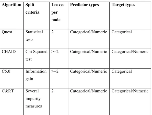
The central point in building a decision tree is the choice of the split attribute. There are several split criteria as shown in Table 1.1-1. The simplest split criteria is as this: Select an attribute, Ai, (to simplify lets consider all attributes and target are binary) and divide the data in 2 sets: one where Ai is 0 and other where Ai is 1. For first set let y0 be the most common value of the target value in it. For second set define y1 the same way. The number of errors by choosing Ai as the split attribute is then the number of examples where the target value is different from y0 and y1 in the respective sets. The selected attribute at each step is the one that minimizes this error.
The described split criteria is very simple and doesn’t give very good results. Other split criteria are shown in Table 1.1-1. To know how they work please read chapter 3 of [1.1-7] and section 3.2.1 of [1.1-4].
Figure 1.1-2 Sample decision tree (taken from [1.1-11])
Understanding a decision tree is straightforward. At each node, starting by the root node, some attribute is being tested. If it is of a certain value we follow a certain branch of the tree, if not we follow other branch. This is done recursively until a leaf node is reached. At a leaf node a certain prediction is made. One can easily rewrite a decision tree as a set of if-then rules to improve its readability.
The main advantage of a decision tree is precisely its readability (in opposition to a neural network where a human cannot understand the reasoning behind a prediction).
Algorithm Split
criteria
Leaves
per
node
Predictor types Target types
Quest Statistical tests
2 Categorical/Numeric Categorical
CHAID Chi Squared
test
>=2 Categorical/Numeric Categorical/Numeric
C5.0 Information gain
>=2 Categorical/Numeric Categorical
C&RT Several impurity measures
2 Categorical/Numeric Categorical/Numeric
Table 1.1-1 Decision tree algorithm comparison
Improving accuracy through boosting
Boosting consists of building several models -the number of models to build is a parameter of the boost mode- each one specialized in the records the previous model failed to classify correctly. The whole set of models is the final model and a voting system is used to decide the final prediction. Boosting frequently improves the accuracy but takes much longer to train.
1.2 Protein Background
Proteins are organic molecules composed of subunits called amino acids. There are twenty different amino acids types available in proteins (list in Appendix B, AII. 1). Amino acids are connected to make proteins by a chemical reaction in which a molecule of water (H2O) is removed, leaving two amino acids residues (i.e. the part
of the amino acid that is left when the water molecule is removed) connected by a peptide bond. Connecting multiple amino acids in this way produces a polypeptide [1.2-7]. A protein might be composed of several polypeptides (i.e. chains).
Figure 1.2-1 Process of connecting amino acids (picture adapted from [1.2-7])
Figure 1.2-1 shows the process of connecting amino acids as has been described above. As we will see during this thesis, amino acids are mainly divided in two categories, hydrophilic (i.e.: tend to be in contact with the solvent) and hydrophobic (i.e.: avoid being in contact with the solvent).
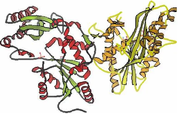
Figure 1.2-2 Image of protein with pdb_id 1n2o
Proteins are an essential part of any living organism and they participate in every process of a cell, many of them being enzymes catalyzing chemical reactions.
The amino acid sequence (simply a string of single letters) is called the primary structure of a protein and uniquely determines the folding of the protein. The final folded shape of a protein (its tertiary structure) is strongly correlated with the protein function in the organism.
One of the major open problems in biology is precisely how to determine the folding of a protein given its amino acid sequence. The solution for this problem will cause a revolution in biology and medicine as it make possible to develop custom assembled proteins to achieve certain functions.
For simplicity, during this thesis, we will often use the term amino acid when technically we should have used the term amino acid residue.
1.2.1 Methods of Structural Classification of
Proteins
Proteins have structural similarities with other proteins. That fact created the necessity of developing methods to classify proteins according to their structure.
There are three main structural classification techniques (SCOP, CATH and Dali). In [1.2-6] an exhaustive comparison between the three is made:
• SCOP (Structural Classification of Proteins) is manually maintained by a group of experts.
• CATH (Class Architecture Topology Homologous) uses a combination of manual and automated methods to define and classify domains.
• Dali (Distance mAtrix aLIgnement) is a fully automated method to define and classify classifying domains.
It is known that automatic assignment algorithms cannot identify all structural and evolutionary relationship between proteins. In this work, we have opted for SCOP because it is considered the more reliable classification method and the “de facto” standard. The release of SCOP used on this thesis was 1.67 from February 2005.
1.2.2 About SCOP
Protein chains in SCOP appear as leafs of a tree with four levels. The levels of the hierarchy are, in this order: class, fold, super family and family. These hierarchy levels pretend to reflect the structural and evolutionary similarities between the proteins.
As quoted from [1.2-10], the major levels in the SCOP hierarchy are:
• class - a very broad description of the structural content of the protein.
• fold - broad structural similarity but with no evidence of a homologous relationship.
• superfamily - sufficient structural similarity to infer a divergent evolutionary relationship but no detectable sequence similarity.
• family - significant sequence similarity.
There are 11 SCOP classes: a, b, c, d, e, f, g, h, i, j, k and l. Each class describes the major structural characteristics of its proteins. Below is the characterization of each of the 11 classes, as quoted from [1.2-10]:
a) proteins with only α-helices b) proteins with only β-sheets
c) proteins with both α-helices and mainly parallel β-sheets (as beta-alpha-beta units)
d) proteins with both α-helices and mainly anti parallel β-sheets (as separate alpha and beta domains)
e) multi domain proteins
f) membrane and cell surface proteins and peptides (not including those involved in the immune system)
g) small proteins with well-defined structure h) coiled-coil proteins
i) low-resolution protein structures j) peptides and fragments
1.2.3 PDB Files Format
PDB is one of the most used formats to store molecule structure related data. It’s a semi structured text file and its format is described in [1.2-5]. A PDB file specifies the position in space of every atom of every amino acid of a given molecule. A protein is a special case of molecule that we are interested in this project.
Figure 1.2-3 shows the beginning of a pdb file.
Figure 1.2-3 Excerpt of the header of 1hvr pdb file
The first rows of a pdb file describe generic information about a protein. The first column of a pdb file describes the type of the row that follows. For instance, the
HEADER row contains the name of the molecule and the date it was deposited at the Protein Data Bank and the EXPDTA row contains the experimental technique used to obtain the protein.
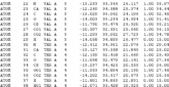
Figure 1.2-4 Excerpt of the body of 1hvr pdb file
The second column in an ATOM row is the atom number, the third column the atom description, the fourth column the three letter amino acid name, the fifth column the chain letter and the sixth column the amino acid number (not necessarily sequential).
Sometimes a letter follows the amino acid number, which we refer as the
CodeResid column. It is this column in conjunction with the amino acid number that uniquely identify an amino acid inside a pdb file because, although rare, in a pdb file two amino acids may have the same amino acid number but different
CodeResids.
The seventh, eighth and ninth columns are the X, Y and Z coordinates of the atom inside the molecule (in angstroms). The last two columns are the occupancy and temperature factor.
In early 2005, when we started the loading process of the pdb files, there was already a beta version of this format in XML. The reason we have choose the txt format was because, despite its problems, it still was better documented. Besides, it occupies much less disk space and is much faster to parse and load.
crystallographic symmetry operations (e.g. : rotations, translations) can be applied to generate a unit cell. The unit cell is the component that is stacked multiple times to generate the entire crystal.
The pdb files we will use during this thesis are biological units (the macromolecules that are believed to be functional). A biological unit (biounit) pdb file is derived from the original asymmetric unit and might be part of the asymmetric unit, the whole asymmetric unit or several asymmetric units. A complete explanation of biological and asymmetric units can be found in [1.2-11].
In sub section 2.1.2 we will thoroughly explain the loading process of the pdb files into our database.
1.2.4 Definition of Secondary Structure of
Proteins
DSSP stands for Definition of Secondary Structure of Proteins. It is a widely used program to calculate, among other things, the secondary structure (e.g. : alfa helix, beta sheets) of a pdb file. It is available for several platforms from [1.2-1] and is free for academic purposes.
DSSP receives as input a pdb file and outputs a dssp file with information about each amino acid. For each amino acid the DSSP program computes its accessible solvent area (the value we are most interested in this thesis), the secondary structure element to which it belongs, the angles the amino acid forms with its predecessor and successor.
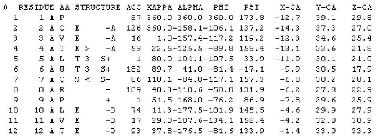
Figure 1.2-5 Excerpt of DSSP classification for 1hvr pdb
In order for the figure to fit the page width, we have eliminated some columns that we do not use in our work. For a complete description of the DSSP output file format please read [1.2-2].
The first column of the DSSP file is a sequential amino acid number, the second is the pdb amino acid number, possible followed by a CodeResid letter. The third column is the chain letter and the fourth column the single letter amino acid code. The fifth column is also a single letter representing the motif to which the amino acid belongs. The most common motifs are H: Alfa Helix (31.8% of all amino acids) and E: Extended Strand in a Beta Ladder (21.8%).
Column ACC contains the amino acid exposed area in Angstroms2, and the KAPPA, ALPHA, PHI and PSI are bond and torsion angles with the neighbouring amino acids. The X-CA, Y-CA and Z-CA columns are simply an output of the coordinates of the alpha carbon atom as found in the pdb file.
1.3 Problem History
The main problem solved in this thesis is the prediction of residue solvent accessibility. This is an interesting problem by itself that can aid in understanding the 3D protein structure.
The initial motivation to tackle this problem was due to the work of other researcher from our group, Marco Correia. In his Master thesis ([1.3-1]) he tested some heuristics to improve the PSICO (Processing Structural Information with Constraint Programming and Optimization) algorithm [1.3-2]. In an important part of his heuristics, the algorithm needs to decide which half of an atom domain should be excluded.
The initial idea behind this thesis was to develop a better heuristic for the placement of atoms inside a protein since the original heuristics only considered geometrical features, not taking into account bio-chemical properties of the atoms or amino acids. Because treating information at the atom level is much more complex than at the amino acid level, we simplified the problem by assuming that all atoms of the same amino acid would have the same burial status of its amino acid.
The burial status of an amino acid is defined as the ratio between its exposed area to the solvent (depends on the protein conformation) and its total area (a constant).
In the literature this problem is called Relative Solvent Accessibility (RSA) prediction. The common values used are twenty and twenty five percent since, from the biochemical point of view, that is the lower bound for chemical interaction.
threshold for comparison with the literature (although, as we will later see why, the results are not directly comparable).
2
Deve lopm e nt of
a Prot e in
Dat a ba se
2
2
In this chapter:
Section 2.1
Loading data
Section 2.2
Cleaning data
Section 2.3
Exploring the database
Section 2.4
Preparing data
Section 2.5
Mining with Clementine
Section 2.6
Chapter Organization
In this chapter we describe the creation of a protein database that contains all the relevant information to solve the problems proposed before. The database, from now on called ProteinsDB, was developed in SQL Server 2005 Developer Edition running over Windows XP Service Pack 2.
The following sections explain the process of building ProteinsDB and the preparation for the data mining phase. We follow the CRISP-DM Methodology described in 1.1.3.
Previous section 1.3, Problem History, roughly corresponds to the first phase of CRISP-DM, the Business Understanding, where the goals for this mining project are described.
Sections 2.1 (Loading PDBs), 2.2 (Cleaning data) and 2.3 (Exploring the database) correspond to the second phase of CRISP, the Data Understanding, where collecting the data, ensurance of data quality and the first insights on the data are performed.
Section 2.4, Preparing data, corresponds to the third phase, Data Preparation, where the requirements and construction of the datasets for mining is described. A specific program with the sole purpose of building these datasets was developed to meet the requirements.
In section 2.5, Mining with Clementine, a description of the data mining stream, starting from the data mining table generated in the previous phase and ending with several models for predicting the burial status of an amino acid is introduced. This roughly corresponds to the fourth phase of CRISP, Modeling.
2.1 Loading data
Loading data into a database is often one of the most time consuming issues, mainly because it is rare that the data might be added promptly to the database without any transformation. This project was no exception and the phase of data loading was particularly time consuming due the amount of data to load and because the not so friendly format of some data sources. There are four main data sources: Tables with amino acid information, PDB files, the DSSP program and the SCOP 1.67 table.
The following sections describe the process of loading those several sources.
2.1.1 Loading amino acid information
As shown before, proteins are composed of sequences of amino acids, and there are twenty different amino acids types. Each amino acid type is described, more or less accurately, via a number of different features. For the purpose of this work we have used two amino acid information sources.
The first source, [2.1-1], is very simple and has only six properties for each amino acid (Hydropathy, Polarity, H_Donor, H_Acceptor, Aromaticity, Charge at Ph7). This data was loaded to table Aminoacids. We will refer to these features of amino acids as information Simple.
The second, [2.1-2], is the most complete we found and has 37 properties (full list in Appendix A, Figure A-8) for each amino acid. This data was loaded to table
Aminoacids_Complete. We will refer to these features of amino acids as information Complete.
Recall that the main aim of this thesis is to predict the Residue Solvent Accessibility (RSA) exposure state. RSA is simply the ratio between Residue Exposed Area (REA) and Residue Total Area (RTA). REA varies with the position of the amino acid inside the protein (and is one of the outputs of DSSP) and RTA is roughly constant for each of the twenty amino acids types.
To calculate the residue total area (RTA) of an amino acid, most papers in the literature use their surface areas available in several tables. However, each table has its own values. For instance, in papers [4.1-2], [4.1-4] and [4.1-1], RTA values are taken from experimental data published on the 1970s or 1980s (Shrake and Rupley(1973) [2.1-3], Chotia(1976) [2.1-4],and Rose et al(1985) [2.1-5] respectively).
We have opted not to use any of those tables and calculate the RTA using also DSSP because all papers consensually calculate REA with DSSP. We calculate the RTA values by using DSSP in a special way. As said before DSSP gives the exposed area of an amino acid inside a protein (which is given in a PDB file). We developed a program to parse a pdb file and, for each amino acid present, isolate it to a new pseudo pdb file. Then, by running DSSP on those new small pseudo PDB files, we have, among other things, the exposed area to the solvent of the selected amino acids (the value is not constant because the amino acid might be taken from different conformations). This computation is performed for many amino acids taken from about two hundred randomly selected pdb files. The results are then averaged to find the solvent accessibility area for each amino acid type.
The fact that each paper uses its own amino acid area tables and data sets makes the prediction values not directly comparable. Regarding the PEA level, however, for papers using amino acid area with table [2.1-4], like [4.1-4], as the denominator for the REA calculation it is possible to do some indirect comparison. Since the values in table s surface area are about 1.7 times smaller than the solvent accessible areas, our percentage of exposed area (PEA) roughly corresponds to other papers PEA/1.7. For instance, if other papers are using a 20% PEA value, we should compare it with our 11.7% PEA level (our closest PEA level is 10%).
In Table 2.1-1 we summarize the results of the described computations, with also the Relative Frequency of each amino acid and the Minimum, Maximum and Standard Deviation of the solvent accessible areas.
A. acid Rel. Freq. Min SA Max SA Avg SA Std. Dev SA [2.1-4]
ALA 8,8% 189 234 214 2,02 115
ARG 5,5% 188 379 352 15,01 225
ASN 4,9% 213 300 275 6,54 150
ASP 6,3% 212 293 274 5,84 160
CYS 1,0% 234 266 243 3,41 135
GLN 3,7% 192 324 303 8,99 190
GLU 5,8% 211 328 301 11,75 180
GLY 7,7% 185 214 191 2,76 75
HIS 1,9% 289 326 302 4,28 195
ILE 5,3% 213 302 281 4,33 175
LEU 9,7% 267 312 285 3,73 170
LYS 7,2% 210 351 315 13,78 200
MET 2,4% 212 323 298 5,87 185
PHE 3,7% 305 337 321 4,6 210
PRO 3,3% 213 266 243 2,96 145
SER 5,4% 211 257 234 3,15 115
THR 6,1% 214 278 254 3,26 140
TRP 1,6% 344 379 363 5,5 255
TYR 3,9% 211 362 343 6,23 230
VAL 5,9% 213 277 257 2,83 155
Table 2.1-1 Amino acids area statistics
We can confirm that the standard deviation is small which indicates the average area is a good approximation of the correct area. All these indicators were added to the Aminoacids table although only the Average Solvent Accessible Area (ASAA) will be used on calculations. The ASAA here forth is a synonymous for the amino acid exposable area and is the denominator in the percentage of exposed area (PEA) equation: Current amino acid accessible area to solvent/Total amino acid accessible area to solvent.
2.1.2 Loading PDBs & DSSPs
The source for the pdb files was the Protein Data Bank (www.rscb.org). We did a local mirror from their FTP server (ftp.rcsb.org) in April 2005. The mirror gave us about 20 gigabytes of compressed data. From those 20 gigabytes, for the context of this work, we are only interested in the biological units (available here:
ftp://ftp.rcsb.org/pub/pdb/data/biounit/coordinates/all). These biological units, as of April 2005, were 5.24 gigabytes of compressed data and about 35.000 files, each file representing a bio unit (a protein or a protein complex).
The file name of a protein file is of the form PDB_ID.pdbX, being pdb_id the four-letter code of the PDB and X a variable we called biounit_id, which is usually 1. Only 30% of the pdb_ids have more than one bio unit.
To load the DSSP information we do not need any of these CSV files or tables. It just requires as input the original pdb file. The output of the DSSP program is a text file (its format was already presented in sub section 1.2.4), which needs to be parsed to be added to the database. We did a simple parser that converts that text file into a CSV file in order to be then easily loaded to the database.
To load the set of CSV files to the ProteinsDB, we have used the SQL Server 2005 command line utility, BCP (Bulk Copy Program), which is quite efficient. To make the loading more efficient we have also turned off the foreign key constraints on the tables involved in this process. The total loading time for a pdb file is highly dependant on the protein size, but on average, it takes about 0.3 seconds, with DSSP being responsible for the majority of the cpu time. The loading itself is mainly an I/O bound task with little cpu overhead.
After all the pdb files are loaded, so is the majority ProteinsDB. The database occupies about 15 gigabytes, with the pdb_data table just by itself occupying near 14 gigabytes. It has approximately 217 million rows, each describing one atom of some amino acid. The dssp_data is the second largest one with near 800 megabytes. It has approximately 12 million rows, each describing an amino acid.
The remaining tables are very small compared to these two. Chain_Headers has 55.476 rows with one per chain and PDB_Headers has 29.841 rows, one per PDB (these numbers do not consider the new pdb files loaded in June 2006 for validation purposes).
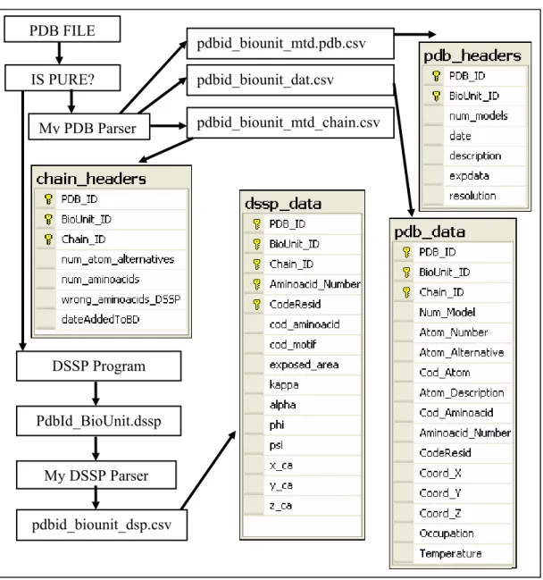
My PDB Parser PDB FILE
pdbid_biounit_mtd.pdb.csv
pdbid_biounit_mtd_chain.csv pdbid_biounit_dat.csv
My DSSP Parser DSSP Program
PdbId_BioUnit.dssp
pdbid_biounit_dsp.csv IS PURE?
Figure 2.1-1 Scheme of processing a single PDB File
For the main purpose of this project, to build a model to determine if an amino acid residue is buried or exposed inside a protein, the pdb_data table is not needed. Nevertheless, this table can be of great use for other projects where information at the atom level is required.
2.1.3 Loading SCOP
SCOP is available as a set of four text files: dir.des.scop.txt_VER,
dir.cla.scop.txt_VER, dir.hie.scop.txt_VER and dir.com.scop.txt_VER with VER
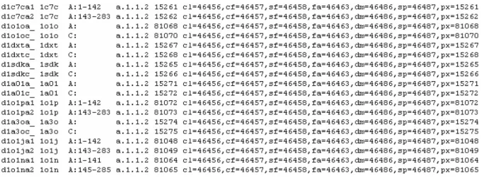
being the name of the scop version. The only file that we need to parse is the classification file-dir.cla.scop.txt. The figure below shows an excerpt of it.
Figure 2.1-2 Excerpt of the SCOP dir.cla.scop.txt_1.67 file
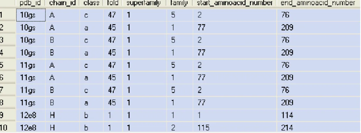
Each line of the scop text file represents the classification of an interval of amino acids inside a chain. The first column is a string with six characters identifying the line, but we will ignore it. The second column is the four letter PDB code (the pdb_id column in our tables), the third column is the chain letter (the chain_id column) plus an optional amino acid interval. Finally, in the fourth column, there are, separated by dots, the class, fold, super family and family classification.
In the third column, after the two dots ‘:’ following the chain identifier, there might be, the amino acid interval for which the family classification applies. If no interval is specified, the family classification applies to the whole chain, which is the more common situation.
Since the scop file is ordered by family classification, Figure 2.1-2 does not show cases where the same chain belongs to different families. We will illustrate those cases, along with further comments to scop, in section Cleaning data.
The cl, cf, sf, fa, dm and sp.numbers are not relevant to our problem but we still loaded them because they might be useful in further projects supported by this database. These numbers are related to the domain classification of the chains.
The px column is a unique identifier of the scop line and is used as the key for the
SCOP table. The table scheme can be seen in Appendix A, Figure A-4.
We developed a simple parser to convert the scop text file into a CSV file and then this CSV file was loaded to the SCOP table in the database throughout the same procedure described in the previous sub section.
2.2 Cleaning data
At this stage we have the database created and loaded with the needed data but we still need to join and clean the information gathered. The main task is to clean the
scop table and merge it with the dssp_data table. We will describe the process in this section.
Let us consider first the scop table. Recall that there are cases where parts of the chain are separately classified. When that happens, we will call the chain irregular. SCOP 1.67 has family information for 51.376 chains with 40.144 (78.5%) regular and 11.062 (27.5%) irregular. Figure 2.2-1 shows examples of some chains belonging to different families.
Figure 2.2-1 Some chains which have amino acids belonging to different families
What interests us most in SCOP is not the number of chains but more the number of families represented by them. The 51.376 chains in SCOP represent 2.886 families. The subset of regular chains represents 2.302 families, 79.8% of the total number of families.
In SCOP a very small number of chains, 65, appear twice with the exact same information (all columns equal except px). For those cases we eliminated the ones with lower px. In addition, a small number of chains, 157, although regular, appear as belonging to two different families. Figure 2.2-2 shows some regular chains which belong to several families.
Figure 2.2-2 Examples of regular chains that belong to several families
To maintain a one to one relationship between a chain and its family classification, we eliminated those chains from the data mining process. These two steps eliminated 65+2*157 chains, leaving us with 39.765 regular chains suitable for data mining but keeping the 2.302 families. The set of regular chains is available from the database view PureScopChains.
The dssp_data table, as of April 2005, has 54.365 chains, representing about 12 million amino acids. A small percentage of them, about 0.5%, appear as lower case letters in the cod_aminoacid column, which should only contain upper case single letter amino acid codes. In accordance to the DSSP manual, which states lower case amino acid letters mean a SS-bridge Cysteine, these lower case amino acid letters were converted to the upper case letter ‘C’, meaning a Cysteine amino acid.
Of the 54.365 chains present in the dssp_data table, 38.736 are in common with the
This subset of 29.379 chains, from 13.441 different pdbs, represents 1.742 families, which is 72.3% of the total possible families if we had also considered the irregular chains. The suitable pdbs for data mining are available from the database view
2.3 Exploring the database
In this section we aim to explore the database to get better acquainted to the data before entering the core data mining process.
As we have seen from the previous section, there are 29.384 chains belonging to 1.742 distinct families on SCOP v1.67 that are suitable for data mining purposes. The distribution of the chains along these families is not homogeneous at all. Figure 2.3-1 shows the top 10 common families. The count column represents the number of chains that belong to the specified family.
Figure 2.3-1 Top 10 SCOP families of all possible chains for DM
On the other hand, the large majority of those 1.742 families have very few chains representing each family. 1.180 families have less than 10 chains representing it, with 339 families represented by a single chain. Table 2.3-1 shows the class distribution of the suitable chains for data mining.
SCOP Class D C B A G J F H K E I Total
Chains count 364 362 303 289 115 107 75 41 38 33 15 1742
Table 2.3-1 Class distribution of suitable chains for DM
Figure 2.3-2 Visualization of chain A of pdb id 1o1p, which has two equal domains
An interesting insight for the residue solvent accessibility problem is the percentage of amino acids exposed at less than X%. Recall that the percentage of exposed area of an amino acid is given by current exposed area/total amino acid exposable area (see 2.1.1). Table 2.3-2 shows the percentage of amino acids exposed at less than each one of the 2, 10, 20, 25 and 30% thresholds, for all the chains up to April 2005.
Percentage of exposed area 2% 10% 20% 25% 30%
Percentage of amino acids exposed at <= X %
27.48% 48.88% 65.79% 73.17% 79.98%
Table 2.3-2 Percentage of amino acids exposed at <= X% in all chains up to April 2005
Percentage of exposed area 2% 10% 20% 25% 30%
PEAM model accuracy 72.52% 51.12% 65.79% 73.17% 79.98%
Table 2.3-3 PEA model accuracy for all chains up to April 2005
2.3.1 Baseline for residue solvent accessibility
The percentage of exposed area model shown just takes into account the percentage of exposed area and returns a unique answer regardless of the input. The idea of the baseline classifier is to improve it by taking into account the exposition of each of the twenty amino acid types.
In [4.1-2], Richardson and Barlow present a paper with a baseline for residue accessibility prediction models. Their baseline consists in assigning a residue into the particular exposure category in which it is most frequently found, not considering its local surrounding sequence. This baseline is the standard by which the literature measures its results. In chapter Experimental Results, we always present our models accuracy as improvement over this baseline classifier.
The baseline classifier works as follow: given a set of proteins as a dataset, it is split in training and test set as usual. In the training set we determine, for each amino acid, the frequency of its appearing in a certain class (i.e.: exposed/buried) for a certain degree of exposition (2%, 10%, 20%, 25% or 30%). The baseline model simple assigns an amino acid to the class where it appears more often (e.g.: if Alanine appears 60% of the time as exposed in the training set, our prediction for all Alanines in the test set is that they are exposed).
The baseline is hence dependent on the dataset and, more specially, on the cut off value for determining if a residue is exposed or buried. It can be considered as a special, very fast to calculate, classifier that has amino acid information Minimal
and window size equal to zero.
![Figure 1.1-1 Architecture of a feed-forward Neural Network with a single hidden layer (figure taken from [1.1-3])](https://thumb-eu.123doks.com/thumbv2/123dok_br/16519802.735603/32.892.133.658.144.515/figure-architecture-forward-neural-network-single-hidden-figure.webp)
![Figure 1.1-2 Sample decision tree (taken from [1.1-11])](https://thumb-eu.123doks.com/thumbv2/123dok_br/16519802.735603/36.892.138.780.140.607/figure-sample-decision-tree-taken-from.webp)
![Figure 1.2-1 Process of connecting amino acids (picture adapted from [1.2-7])](https://thumb-eu.123doks.com/thumbv2/123dok_br/16519802.735603/38.892.148.532.501.784/figure-process-connecting-amino-acids-picture-adapted.webp)