Ricardo Jorge Palheira Mestre

(1)

Ricardo Jorge Palheira Mestre

Licenciado em Engenharia Informática

Improvements on the KNN Classifier

Dissertação para obtenção do Grau de Mestre em Engenharia Informática

Orientador : Joaquim Francisco Ferreira da Silva, Prof. Auxiliar, Universidade Nova de Lisboa

Júri:

Presidente: Prof. Doutora Carla Maria Gonçalves Ferreira (FCT-UNL)

Arguente: Prof. Doutora Maria da Graça de Figueiredo Rodrigues Gaspar (FCUL)

(2)

(3)

iii

Improvements on the KNN Classifier

(4)

(5)

(6)

(7)

Acknowledgements

The development of this dissertation has been one of the most significant academic challenges I have ever had to face. However, this report represents the culmination of an academic goal to which I dedicated myself and would not be completed without the help of several people.

First of all, I would like to express my deepest sense of gratitude to my Ph.D. advisor, Dr. Joaquim Ferreira da Silva. I thank him for the continuous guidance and great effort he put into training me in the scientific field. His wisdom, knowledge and commitment to archive great goals inspired and motivated me.

I would like to thank my friends and colleagues António Mota, João Luis, João Silva, Nuno Gomes, Patrícia Espada and Tiago Melo for walking me through the process of writing this dissertation, always offering their strength, help, and companionship.

(8)

(9)

Abstract

The object classification is an important area within the artificial intelligence and its application extends to various areas, whether or not in the branch of science. Among the other classifiers, theK-nearest neighbor(KNN) is among the most simple and accurate especially in environments where the data distribution is unknown or apparently not parameterizable. This algorithm assigns the classifying element the major class in the

Knearest neighbors. According to the original algorithm, this classification implies the calculation of the distances between the classifying instance and each one of the training objects.

If on the one hand, having an extensive training set is an element of importance in order to obtain a high accuracy, on the other hand, it makes the classification of each object slower due to itslazy−learningalgorithm nature. Indeed, this algorithm does not provide any means of storing information about the previous calculated classifications, making the calculation of the classification of two equal instances mandatory. In a way, it may be said that this classifierdoes not learn.

This dissertation focuses on the lazy-learning fragility and intends to propose a solution that transforms the KNN into an eager-learning classifier. In other words, it is intended that the algorithm learns effectively with the training set, thus avoiding redundant calculations.

In the context of the proposed change in the algorithm, it is important to highlight the attributes that most characterize the objects according to their discriminating power. In this framework, there will be a study regarding the implementation of these transformations on data of different types: continuous and/or categorical.

(10)

(11)

Resumo

A classificação de objectos é uma área importante no âmbito da inteligência artificial e a sua aplicação estende-se às mais variadas áreas, sejam estas ou não no ramo das ciências. Entre os demais classificadores, o algoritmoK-nearest neighbor(KNN) está entre os mais simples e eficientes especialmente em ambientes onde a distribuição dos dados é desconhecida ou aparentemente não parametrizável. Este algoritmo atribui ao elemento a classificar, a classe maioritária nosKvizinhos mais próximos. Esta classificação implica, segundo o algoritmo original, o cálculo das distâncias entre a instância a classificar e cada um dos objectos de treino.

Se o fato de um conjunto de treino ser extenso é um elemento importante para se obter uma precisão elevada, por outro lado, torna a classificação de cada objeto mais lenta devido à naturezalazy-learningdeste algoritmo. Com efeito, este algoritmo não contempla qualquer forma de guardar informação sobre as classificações calculadas anteriormente, o que torna o cálculo da classificação de duas instâncias iguais, obrigatório. De certo modo, poder-se-ia dizer que este classificadornão aprende.

Esta dissertação debruça-se sobre a fragilidadelazy-learninge pretende propor uma solução que transforme o KNN num classificadoreager-learning. Por outras palavras, pretende-se que o algoritmo aprenda efetivamente com o conjunto de treino, evitando assim, cálculos redundantes.

No contexto da alteração a propor no algoritmo, torna-se importante valorizar os atributos caracterizadores dos objetos segundo o seu poder discriminante. Neste enqua-dramento, será ainda feito um estudo com vista à aplicação destas transformações em dados de diferentes naturezas: contínuos e/ou categóricos.

(12)

(13)

List of Figures

2.1 Removing outliers and creating the final training set. . . 7

2.2 Accuracy values using differentεthresholds using 80% of the samples as the training set. . . 7

2.3 Centroid-Based Document Classifier (CBDC) Vs. Removing Outliers (RO) comparison. . . 7

2.4 Misidentified outlier example.. . . 8

2.5 Inappropriate threshold example. . . 8

2.6 SSR Tree structure. . . 11

2.7 Classification time comparison on 1000 samples. . . 11

2.8 Identified Core Set examples. . . 12

3.1 Data structure division step. . . 16

3.2 Simple dataset with fifteen samples over two dimensions and three classes. 16 3.3 Fixed Grid structure using three intervals. . . 17

3.4 QuadTree structure example. . . 19

3.5 KD-Tree structure example. . . 20

3.6 InTree structure example. . . 21

3.7 Different attribute set discriminant power example. . . 22

3.8 Eye color attribute transformation axis. . . 26

4.1 Data structures classification times. . . 34

4.2 Data structures learning times. . . 34

4.3 QuadTree classification test1s using HDH.. . . 34

4.4 QuadTree classification tests using HDH. . . 34

4.5 QuadTree classification tests using SDH. . . 34

4.6 QuadTree classification tests using normalized data and HDH.. . . 35

4.7 QuadTree classification tests using normalized data and SDH. . . 35

4.8 KD-Tree classification tests using HDH. . . 35

(16)

xvi LIST OF FIGURES

4.10 KD-Tree classification tests using normalized data and HDH.. . . 35

4.11 KD-Tree classification tests using normalized data and SDH. . . 35

4.12 InTree classification tests using HDH. . . 35

4.13 InTree classification tests using SDH. . . 35

4.14 InTree classification tests using normalized data and HDH. . . 36

4.15 InTree classification tests using normalized data and SDH. . . 36

(17)

List of Tables

3.1 Eye color distribution over hemispheres.. . . 24

3.2 Eye color conditional probabilities. . . 25

4.1 Dataset collection features. . . 32

4.2 Classification accuracy for different data structures. . . 37

4.3 RecommendedKvalues for data structures variants. . . 38

4.4 Data structures differences applying attribute weights. . . 39

(18)

(19)

1

Introduction

This chapter introduces the topic of this thesis. It will present the context and motivation of this work. The drawbacks associated to this scope will be detailed, as well as the expected contributions as a consequence of the solutions that will be proposed.

Also the outline of the document will be presented.

1.1 Context

In the context of artificial intelligence, pattern recognition is one of the most interesting topics. By definition, pattern recognition is the science that deals with description and classification of objects [MdS00]. Its application extends to several areas beyond computer science such as psychology, psychiatry, ethology, astronomy, biochemistry, microbiology, physics, etc. Regarding computer science, it is common to find references to several applications such as speech recognition, document classification, handwriting recognition, image processing, etc.

Pattern recognition systems/classifiers are typically analysis of information, compris-ing feature extraction mechanisms to be used in a classification algorithm. The process that selects and analyzes information regarding the characteristics and builds class prototypes is called learning or training [AF03]. The better the attributes are selected, this is, how much they characterize classes, the bigger is the tendency to get them separated in the vector space dictated by the attributes. Training phase is followed by the classification phase which is based on the learning previously built.

(20)

1. INTRODUCTION 1.2. Motivation and Problem Description

minimize errors when classifying new elements later on. Over time, different methodolo-gies have been developed for learning phase, typically being divided into unsupervised and supervised learning.

In the unsupervised learning there is no knowledge of the set of classes or the classes associated with each training sample. This method has the advantage of learning new classes over time. Therefore it can be considered as a dynamic learning with regarding the set of classes. On the other hand, dispensing human supervision normally shows poorer results in the classification phase of new objects.

Supervised learning is distinguished by a set of characteristics: set of classes to analyze it is known à prioriand in the training set, each sample is associated with the class to which it belongs. There are several algorithms that fall under this approach, we highlight the classic Naive Bayes classifier, C4.5, SVM and KNN, the latter being the focus of this dissertation.

1.2 Motivation and Problem Description

The KNN classifier has a very simple philosophy. A sample is classified according to the same class that predominates in itsK closest instances. In addition to their simple implementation, the main advantages are: has few parameters (only the distance and the valueK) and its robustness, supporting noise between classes, this means the classes do not need to be linearly separated, which can be explained for not depending on the distribution model of data, but only from its nearest neighbors. The KNN algorithm is thus a nonparametric classifier. However, KNN as any other classifier has disadvantages. Although withstand noise, the choice of the attributes must be careful. If there are irrelevant or too noisy attributes, they may deviate estimates [Asc03,dat].

The biggest problem of KNN and the main focus of this work has to do with the trend that this classifier has to be slow. This feature is due to the fact that the KNN classifier is a lazy-learning algorithm since for classifying each instance it needs to calculate the distances to all other known instancesN (training samples). This algorithm has a time complexity of O(N.D) for each classification, being D the number of attributes that characterize. This is especially problematic for large data sets and/or with a large number of attributes. In a sense, we can consider that this classifier does not learn, since it can not take any advantage of the classifications already made, as alike as the elements to be classified are.

Besides the disadvantage lazy-learning, another problem of this algorithm is in the data types that it tries to classify. As we know, the KNN classifier is based onKnearest neighbors, but the concept of "nearest" may have different points of view. If the training set contains data characterized by continuous attributes, it is natural that the distance between two samples refers directly as Euclidean distance. However there is room to improve the set of attributes that characterize the training set. One of the typical ways consists in assigning different weights to the attributes as the discriminating power of

(21)

1. INTRODUCTION 1.3. Outline of the Document

each. Although there are already several approaches for assigning weights, these may or may not be appropriate in the context of the solution that will be proposed to minimize the lazy-learning problem.

Often it is up to the algorithm to deal with discrete data. This type of data can also be ordinal or nominal/categorical. This first type of data refers intervals continuous values (eg ranges of heights, weights, etc.) and so, if the attribute is informative enough, the Euclidean distance can be applied. However, categorical data values do not refer nor quantitative or qualitative categories (eg blood type, race, etc.), getting the Euclidean distance apparently inadequate. Typically, the difference between two instances containing categorical information is equal to the number of attributes that contain different values. Although this is a way to find differences, this may not show correctly how different two samples really are.

In order to address this problem, it will be developed a solution that seeks to establish the notion of distance between subcategories of each categorical attribute.

1.3 Outline of the Document

Chapter2highlights three types of issues associated with the KNN algorithm. "State of art" approaches are presented as previous research on those subjects is analyzed, revealing their flaws.

In Chapter3we discuss the challenges to overcome the previously exposed weaknesses. Also, solutions are outlined and their processes are detailed.

Chapter4focuses in testing previously discussed solutions. Datasets are presented in4.1and in Subsections4.2,4.3and4.4test and performance results of our proposed approach are analyzed and interpreted.

(22)

1. INTRODUCTION 1.3. Outline of the Document

(23)

2

Related Work

Given the weaknesses of the KNN classifier due to its nature, the "state of art" may be divided into three areas: a) training sample reduction; b) changing the weight of attributes and the weight of vote; c) minimization of the lazy-learning problematic.

In general, the approaches regarding a) attempt to summarize the training set into a minimum number of representatives. The idea is to minimize the inherent computational work in the classification phase of new elements. The proposals regarding b) try to incorporate as informative only attributes with discriminating power, sometimes assigning different importance to different attributes. In addition, each nearest neighbor voting weight may not be the same. For group c) approaches try to reduce the searching space commonly by using tree structures, trying to group elements with similar characteristics, improving classification time without penalizing accuracy levels obtained in the KNN original solution.

While this review may be not exhaustive regarding to all existing documents since the KNN algorithm was designed, it is complete for the three areas in which this algorithm can be improved. I tried to do it by analyzing the most recent work in this area as these would naturally accumulate all the improvements up to date.

2.1 Reducing the Training Sample

In [SAH06], authors proposed an approach for classifying documents by eliminating training sample outliers in oder to obtain more accurate classifications. Outliers are elements that deviate significantly from the normal pattern of the class to which they belong.

(24)

2. RELATEDWORK 2.1. Reducing the Training Sample

[HK00] to obtain the centroid of each class.

In centroid based classification algorithm (Centroid-Based Document Classifier), doc-uments are represented using vector-space model. In this model, each documentdis represented by a vector of terms/keywords. These terms are typically words with dis-criminating power. In its simplest form, each document is represented by the term-frequency vector (TF)dtf = (tf1, tf2, . . . , tfn), wheretfi is the ith term frequency in the

document. This model has been refined to weigh each term throughInverse Document Frequency(IDF) in all training documents set. This is done by multiplyingtfibylog(_dfNi),

where N is the number of total of training documents, and dfi the number of

docu-ments that containithterm. Thus, the vector-space model assumes the following form:

dtf idf = (tf1log(_dfN₁), tf2log(_dfN₂), . . . , tfnlog(_dfNn)). In this model, the similarity between two

documentsdianddjis measured using the cosine metric:

cos(di, dj) =

di.dj

||di||2× ||dj||2 (2.1)

where "." denotes, in this case, the inner product of two vectors. Once the document vectors are previously normalized to length 1, Equation2.1can be simplified to:

cos(di, dj) =di.dj (2.2)

The centroid of a class is defined by:

Cc = 1

||Sc||

X

d∈Sc

d (2.3)

whereScis the set of representative vectors of class’ documents. Thus, the centroid is a

vector obtained by averaging the weights of the different terms in class’ documents.

The distance between each class’ centroid and the document vector is computed through Equations2.2and2.3. According to the authors, it was observed that the ele-ments that are too far from the centroid of its class (outliers) may reduce accuracy when classifying new elements. Therefore, those elements should be discarded in order to form a new training set.

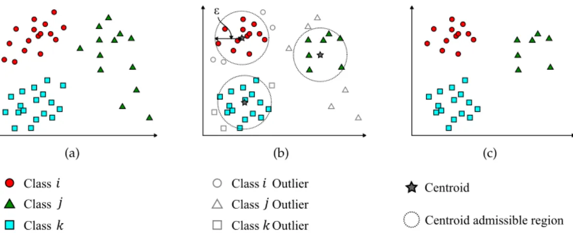
To determine which documents should be considered outliers, the authors established a threshold ε, after several experiments. Figure 2.1 shows the sequence of steps for obtaining the new training set, as Figure 2.1(a) illustrates the initial set; Figure 2.1(b)

outliers identification; and Figure2.1(c)the new training set.

Having this new training sample, the original KNN rule is applied, that is, identifying the majority class in theKnearest documents of the document being classified.

In the particular case of the centroid classification-based approach [HK00], the final set of training is reduced to the set of centroids. Thus, this approach can be viewed as a KNN technique in whichK= 1.

(25)

(a) (b) (c)

Figure 2.1: Removing outliers and creating the final training set.

Figure 2.2: Accuracy values using differentεthresholds using 80% of the samples as the training set.

(26)

The obtained results for the different threshold values are shown in Figure2.2. Fig-ure2.3evaluates the impact of removing the outliers in the Centroid-Based Document Classifier.

This approach has three drawbacks: it is inadequate for multimodal distributions; the threshold value may not be suitable for different densities, and classification remains being lazy-learning.

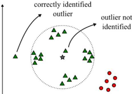
Figure 2.4: Misidentified outlier example.

In the case of each class having multimodal distributions in the vector space as shown in Figure2.4, it is possible that some outliers are not identified as such. The element next to the centroid of the class identified by triangles would never be identified as an outlier once it is very close to the centroid. However, the leftmost element is correctly identified as an outlier.

Figure 2.5: Inappropriate threshold example.

Figure2.5shows the same threshold (illustrated by the circle) is inadequate to detect outliers in both classes. It is easy to accept that elements outside the circumference should not be considered outliers, as there is a balanced distribution between those four elements relative to the class’ centroid. Furthermore, the threshold value is obtained empirically for each training set as there has not been developed any automatic way to compute it.

Finally, for each new instance to be classified, it is still necessary to compute the distance between the element to classify and all training samples, leaving the lazy-learning issue unsolved.

In [ZTD12], the authors propose reducing the number of training samples by introduc-ing the "Essential Vector" which is a mechanism that is not clearly explained. However,

(27)

2. RELATEDWORK 2.2. Changing Attributes Weight and its Vote Weight

according to the authors, the gains in reducing the complexity are significant. Still, the results only address one specific area: documents classification. There is no reference on applying this approach in numerical Vs. categorical attributes.

2.2 Changing Attributes Weight and its Vote Weight

In [AKS], the authors use theApriori– a Data Mining algorithm for automated association rules extraction – in order to improve the initial set of attributes quality, selecting a subset of them that are able to continue to characterize and discriminate training/learning objects’ classes. In other words, considering that in the classifier learning process, the training objects are usually characterized by a set of attributes/features that may contain some redundancy (wholly or in part), it would be beneficial that the number of attributes could be as reduced as possible. Indeed, if there is a mechanism which is able to select a subset of those attributes in such way that the objects’ classes remain discriminable, the classification training and classification processes will be faster and more simplified.

In the particular case of KNN, given the nature of this classifier, such attribute reduction is reflected by a time efficiency improvement only in the classification phase. In this phase, the object being classified has to be compared with all the training objects since this classifier does not build patterns for each known class.

The approach presented in [AKS] selects the "Prominent Attributes" that best character-ize the classes and assigns them a weight according to its importance. According to the authors, there were performance increases up to 40%. This improvement was observed especially in classification accuracy compared with the original KNN where all attributes have the same weight, which sometimes causes misclassifications.

This approach may provide significant improvement for most classifiers. However, if the initial attributes in a set of objects contain no redundancy and they have similar discriminating power, this approach will not benefit KNN as this classifier biggest disad-vantage relates to its lazy-learning nature. In other words, the improvement shown in this approach does not avoid that each object has to be, still, compared to all training elements, which makes it extremely inefficient in cases where the set is very large.

As in [AKS], other authors, for example [PSFA11], propose improvements in the scope of attribute’s weight for computing the distance between the object to be classified and the training elements. One of the first proposals is in [SA76]. In this paper, the author introduces the method of weighting votes (WKNN), where the nearest neighbors are given more weight than the farthest ones by using the weighted distance function. Thus, for a chosenKvalue, the weight assigned to theithneighbor follows three steps: it computes the distance from theKth _{neighbor to the object being classified, lets call it} _A_{; the it}

(28)

2. RELATEDWORK 2.3. Minimizing the Lazy-Learning Problematic

determination. In some cases, WKNN got some improvements compared to the original KNN.

In [ZWZZ07], the authors propose a method they callKernel Difference-Weighted Nearest Neighbor(KDF-WKNN). This method defines the KNN rule as a constrained optimization problem. The authors also propose an efficient solution to compute the different nearest neighbors weights according to their distance to the object to be classified. According to the authors, the KDF-WKNN performs better than the original KNN and WKNN, and it is comparable to some of the "state of the art" methods in terms of classification accuracy.

In [GDZX12], the authors developed a new KNN rule namedDistance-Weighted K-Nearest Neighbor(DWKNN). The motivation for it lies on the problem of the sensitivity of the K value when using KNN classifier, aiming to improve accuracy results. The results presented by the authors show robustness regarding the chosenKvalue and good accuracy when compared to other KNN approaches.

Previous approaches ([AKS,SA76,ZWZZ07,GDZX12]) are proposal examples to com-pute the distances in order to improve the KNN’s achieved accuracy, either through filtering the best attributes, or by assigning weights based on distance for voting pur-poses in the class assignment. However, regarding the accuracy obtained, even in the original version, this classifier is comparable to the best ones in some environments, even managing to overcome some, particularly in circumstances where it is difficult to obtain data distribution models in the vector space defined by characterizing attributes. Also, these approaches do not offer any solution for the biggest disadvantage of KNN when compared to other classifiers, that is, its lazy-learning characteristic.

2.3 Minimizing the Lazy-Learning Problematic

In [WW07] a solution to minimize the lazy-learning problem is proposed. The presented TFKNN method can quickly find theKnearest neighbors. The algorithm uses a SSR tree data structure (a type ofB+−T ree) where each non-leaf nodes are classified according to the distance between its centroid and its parent’s centroid. With this structure, it is possible to reduce the search scope, and hence the computation time. We may take an example of this structure in Figure2.6.

The tree structure is as it follows:

• A non-leaf node is a minimal region that contains all its child nodes;

• All leaf nodes are at same depth and each leaf corresponds to an individual training sample;

• A non-leaf node represents a training set that contains: centroid, radius, distance between parent node and itself; pointer to parent node; number of children and pointers to them;

• Besides the sample, a leaf includes the distance and the pointer to its parent node.

(29)

Figure 2.6: SSR Tree structure.

The tree must satisfy the following conditions:

• Root node has at least two child nodes, unless it is a leaf itself;

• All non-leaf nodes have a number of children between a pre-defined minimum and maximum;

• All non-leaf nodes are sorted in ascending order of distances between their centroid and its parent’s center point.

Selecting theK closest elements is performed by seeking through the tree taking into account the closest nodes to the object being classified.

Figure 2.7: Classification time comparison on 1000 samples.

Figure2.7shows important improvements in classification time when compared to the original KNN andarray-indexKNN [YW05] (which is a method that uses the KNN rule applied to afuzzy decision tree). However, the authors state that this approach needs to be improved in terms of classification accuracy, which suggests a decrease in performance at this domain.

The authors do not mention the problem regarding the nature of the attributes (cate-gorical Vs. numerical) in the context of this approach.

(30)

the same class, then it would not be necessary to divide further down and the subsequent searches would be faster.

In [Jua11], the authors propose a tree approach in order to minimize the lazy-learning problem, the TKNN. The algorithm characterizes the training elements based on the highest similarity that separates the training set inCore Sets, thereby reducing the search range. Tree nodes correspond to each training set elements’ average, in each core, being its elements close enough, according to the Euclidean distance. When a new training element comes up, the algorithm decides which Core Set it belongs to; the decision may result in the creation of a new Core Set.

Different sequences of scanning training set elements may end up building different trees. One of the objectives of the approach is to be able to build compact trees. TKNN’s accuracy depends on the distance’s radius value which was set initially and it is a param-eter that influences the number of Core Sets. The tree nodes are therefore the Core Sets that belong to different regions, each one characterized by elements near to each other. Thus, different regions distribution determines tree structure and consequently its search efficiency in the classification phase.

In order to ensure a good performance, training samples are used to estimate the best radius distance to be used.

According to the results, in some tests, TKNN shows better accuracy values; but slightly worse for some data sets. The algorithm takes linear time proportional to the training set size.

In my point of view, this approach has a drawback: if class distribution is not separated enough in the vector space, each Core Set will represent a region containing multiple classes elements, which would lead to misclassifications as is shown in Figure2.8. The Core Set depicted by the lower circumference contains elements of more that just one class could result in subsequent misclassifications.

Figure 2.8: Identified Core Set examples.

An algorithm is presented in [PQS04] that aims to improve the original KNN’s accu-racy and which scope is the pattern recognition in image domain. This technique uses an important toolMean Vector, which is used to reduce the search range. The core idea of this approach focuses on rejecting vectors that are impossible to be included in theK

(31)

2. RELATEDWORK 2.4. Resume

closest vectors set. Thus, classification time is reduced and the accuracy of the classifi-cation keeps close to the original KNN, according to the authors. Basically, to find the

Kclosest elements, the original vectors are transformed byHaar Waveletand sorted by theirApproximate Coefficients(the Mean Vectors) calculated in the same Wavelet scope - see [PQS04] for more details. To extract image features, the spline wavelet is used. According to the authors, when the size of features vector is not a power of 2, the length of the vector transformed by Haar Wavelet increases, which implies the need for more computational memory. The authors do not discuss the potential application of this technique in different contexts rather than images, taking into account the attributes of different data types (numerical Vs. categorical).

2.4 Resume

Given the weaknesses mentioned in the introduction of this chapter and the solutions proposed by different authors, the following should be emphasized:

(a) The training sample reduction proposals may lead to misclassification, especially in the cases where class boundaries are not well defined. However, in many cases, it ends up by improving classification. This group of solutions does not aim to solve the lazy-learning problem;

(b) In the scope of weighted attributes, the proposed solutions are efficient if the attributes are expected to have different discriminant capabilities or there is some redundancy between them; but only in these cases. Regarding the efficiency of assigning weight to votes depending on the distance of nearest neighbors, we can say that in cases where the training set is distributed into clearly separated class’ clouds, these techniques minimize the sensitivity regards the user’s selectedKvalue. In fact, if the classes are clearly separated, for anyKchosen value, there is a tendency for the nearest neighbor to determine the class assignment, since it got the most weighted vote, hence reducing theK value sensitivity. However, this weight assignment becomes detrimental in cases where the quality of the attributes does not allow a clear classes distribution into separate clouds. In short, the impact of assigning weights to attributes is highly dependent on the quality of the attributes. This class of solutions does not address the lazy-learning issue, as well;

(32)

2. RELATEDWORK 2.4. Resume

attributes of different natures (categorical, numeric, . . . ). This issue is not mentioned by the authors.

(33)

3

Improving KNN – Solutions

Considering that the original KNN does not use previous classifications as a learning source, this algorithm tends to be very inefficient when working with large data sets, as it was mentioned before.

In order to cope this problem, providing KNN algorithm some intelligence, we consid-ered a set of alternative structures organized in order to implement a learning (training) phase. Although this training phase may be heavy, it happens only once for each data set. Then, once this phase is completed for a given data set, the performance in the classification phase is highly rewarding.

3.1 Structures to Support the Learning Phase

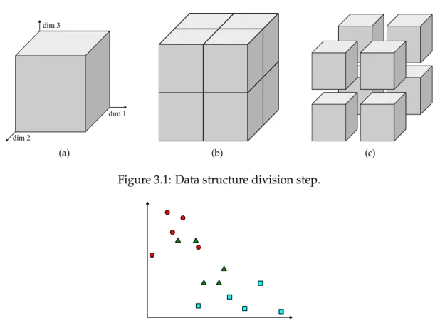
The learning phase consists of two steps: division and pre-classification. In the division, each dataset attribute represents a dimension. The range of each attribute (represented in Figure3.1(a)) is segmented, so the original vectorial space is split successively in smaller blocks (as show in Figure3.1(b)and Figure3.1(c)) while the data structure is created. The final blocks granularity is defined by a criterion which be explained later. In order to conclude the learning phase, each one of those final blocks is associated with a class.

The idea is to divide the vectorial space such that there is a very high probability that each block ispopulatedby elements of just one class.

(34)

3. IMPROVINGKNN – SOLUTIONS 3.1. Structures to Support the Learning Phase

(a) (b) (c)

Figure 3.1: Data structure division step.

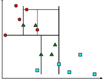
Figure 3.2: Simple dataset with fifteen samples over two dimensions and three classes.

3.1.1 Fixed Grid

The first alternative approach regarding the implementation of an intelligent KNN algo-rithm consists of a rough division of each dimension range as it is divided intoI equally intervals.

Basically, Fixed Grid transforms the dataset into a multidimensional matrix.

3.1.1.1 Learning Phase

After computing interval size for each dimension, the resulting intersections will be represented in aID matrix, which I call pre-classification matrix, whereDis the number of attributes.

As the matrix structure is set, each cell now will represent a region limited through the interval size of each dimension. Each one of those regions will associate a class. This associated class will be the result of classifying the region’s central point using the original KNN. This means, comparing the distances from the region’s central point to the whole dataset and selecting the majority class in theKnearest samples. Thus, the learning-phase space complexity isO(ID)and this phase has anO(ID×N D)time complexity, whereN

is the number of samples in the dataset.

In the example below (Figure3.3) each dataset attribute range is divided in three equal divisions.

(35)

Figure 3.3: Fixed Grid structure using three intervals.

3.1.1.2 Classification

The upside of this structure is the classification-phase time. The classification of a new element (or a sample) involves computing each dimension’s index and accessing the pre-classification matrix. Recall that each pre-pre-classification matrix cell contains an associated class representing the whole cell region. Therefore, classifying a new element is anO(D)

time operation.

Looking at Figure 3.3, if we want to classify a new element whose attributes, for example, point to the top left rectangle[1,3], and(K= 5)is used, its pre-classification will associate the "red circle" class two this new element. Actually, if we were about to classify any sample within this cell region, it would always result in "red circle" for(K= 5).

3.1.1.3 Resume

Although being a very simple way for providing KNN with intelligence, it is also a very rudimentary and rigid method due to its inability to adapt to the dataset. Since every dimension is divided into the same I equally spaced intervals, this does not guarantee that each cell contains a clear majority of elements of the same class. Besides, it may result in contiguous empty cells (having no samples) or it may result in an avoidable over-division of the space when contiguous cells are populated with samples from just one and the same class.

The learning-phase time complexity and the disadvantages mentioned above moti-vated me to research other alternative structures. However, this will be used as base of comparison to other structures.

3.1.2 QuadTree

The QuadTree structure is a first evolution from the Fixed Grid.

As said before, Fixed Grid structures division is susceptible to produceempty divisions

and over-divided regions. In order to solve these problems, a matrix based structure still would not be optimal. To maintain the advantages of the fast indexing regions, this QuadTree solution is based on a tree data structure.

(36)

for each attribute in the data set. Each node represents a region and all dataset samples contained in it. In this structure, a node does not contain child nodes (leaf) either because it does not contain any samples in its region or because its data has what we consider a majority class. When a subset of data consists of high percentage of a given class, it is considered to have a majority class. For this high percentage I choose 99%.

Division is a recursive and breadth-first process that for a node (containing data) will split each dimension in two equal halves, resulting in2D _{child nodes, where}_D_{is the number}

of dimensions. Each one of these child nodes will repeat the process until either it has no data or a majority class arises.

This is considered to be a more efficient method due to its division rules since empty regions will not be divided, therefore there will be no "over-computation". The same happens to divisions where a class is considered to be the major class. In other words, this resolves the problem of the overly divided regions. These two situations are presented in the example at Figure3.4.

After this vector space division phase is finished, a pre-classification phase (similar to the one used in the Fixed Grid) is applied. In this phase, each leaf will be associated to a class. This class may be set by one of the two following ways:

• Simple Distance Heuristic (SDH) – as in the the Fixed Grid structure, each leaf’s central point will be used to compute the distance from itself to each of all data sample; then, as in the case of Fixed Grid, the nearestKsamples decide which class represents the region;

• Hierarchical Distance Heuristic (HDH) – it is similar to SDH, but instead of consid-ering all data samples, it just takes into account theKclosest samples considering the hierarchical structure where the leaf’s central point belongs to. In other words, if the number of samples within the leaf’s region is less thanK, the leaf’s parent level is considered in order to get enough samples (K). If still not enough, this step may be repeated. Again, as in the resulting data samples are used as in SDH to locate the

Knearest ones and the leaf’s class representative.

The process that defines QuadTree structure regions, this is, the dividing phase, takes in average, timeO(N)using SDH heuristic, while its spatial complexity will beO(N). For the pre-classification phase, it takes timeO(LN D), whereLif the number of resulting leafs after division phase. When using HDH, this pre-classification phase is more dependent on the data distribution through classes then the SDH.

To classify a sample is as direct as search through the pre-classification tree. This means the classification of a sample has complexityO(log₂D(N)).

(37)

Figure 3.4: QuadTree structure example.

3.1.2.3 Resume

The main advantage of this QuadTree structure is that it handles regions better, avoiding to over compute either blank or meaningful regions. This results in an improvement on both training and sample classification times.

3.1.3 KD-Tree

As the QuadTree tree structure makes successiveblind divisions, always splitting each dimension in two halves. This isn’t optimal in datasets containing really dense clusters (not containing a majority class). The problem with this is that successive iterations may not be splitting those clusters. KD-Tree structure tries to overcome that brack.

Like QuadTree, KD-Tree is also a tree based structure. The big difference between these structures is the way they divide the dataset attribute ranges. Instead of having each node dividing all dimensions in two halves, each KD-Tree node divides just one dimension at a time based on its dimension subsample mean value. Its child nodes will repeat the process using other dimension.

Each of KD-Tree node has a flag indicating if the node itself is a left or right child, the dimension and value where this node spits the subset and it may have two child nodes.

Like QuadTree, KD-Tree division is a recursive and breadth-first process. Each node computes the contained subset mean value over a given dimension. This value is set to the node and it is used to split the contained subset in two parts. Each one of these child nodes will repeat the process using another dimension until either it has no data or it has a majority class.

This way, even the clusters that might took QuadTrees structure several iterations to start dividing, would be detected and split earlier.

(38)

Creating the tree structure for KD-Tree when using SDH heuristic takes in average timeO(N)as spatial complexity will beO(N). Pre-classifying this tree structure, as in QuadTree, takes timeO(LN D).

In Figure3.5it is possible to notice how divisions are made at each iteration on each axis (dimension). Every division considers the mean value of its dimension/attribute subset.

Figure 3.5: KD-Tree structure example.

Analogously to QuadTree, a sample’s classification is as complex as searching through the pre-classification tree. This means the classification of a sample has complexityO(log₂(N)).

3.1.3.3 Resume

Contrary to QuadTree that may overloop in very condensed clusters, KD-Tree forces its separation in early iterations. Also, because KD-Tree uses dimension’s mean values to split subsets, it does not allow the formation of blank divisions, which results in fewer divisions. These are the reasons why KD-Tree’s learning phase turns to be faster than QuadTree.

We can compare both examples shown in Figure3.4and Figure3.5. Figure3.4resulted in a QuadTree with 22 leafs which 10 have no data in its regions while Figure3.5shows that KD-Tree divided the same set on 11 leafs.

3.1.4 Interval Tree

Although this structure still follows the same ideas as the previous ones, it has a different approach regarding the division phase.

The problem when making divisions in the QuadTree and KD-Tree structures is defining the dividing point on the dataset. Instead of roughly dividing the whole dataset, Interval Tree (InTree) structures tries to divide the set in order to minimize the number of future divisions.

Despite the differences regarding division phase, InTree structure is the same as the KD-Tree as pre-classification and classification phases work the same way. However,

(39)

InTree nodes have three additional informations: a flag indicating if the node itself is a left or right child; the dimension identification and value where it spits the subset. Each node may have two child nodes.

Instead of trying to divide the dataset until it either has no data or it has a majority class, for each InTree iteration, it computes all class ranges at a given dimension. The class whose limit is closer to the dimension’s mean value of the dataset will be used for dividing the set (as shown in Figure3.6). This way, every iteration guarantees at least one class is full contained in one of these new divisions.

As in the previous structures, the final tree structure will be scanned and each leaf will be associated to a class. This association is made as before, using either of the two presented heuristics. This is: either by running the original KNN algorithm, using its leaf’s central point to compute distances to the whole set, or considering the firstK samples in its hierarchy.

Once the InTree is slightly different than KD-Tree, so its division phase is also different and takes timeO(CN), where SDH heuristic is considered andCrepresents the number of classes in the dataset. This difference can be explained by the need of finding the class’ limit which is the nearest one to the dimension’s center on each iteration. The spatial complexity for this phase isO(N). Similarly to QuadTree and KD-Tree structures, pre-classification timeO(LN D).

Figure 3.6: InTree structure example.

Classifying a sample using the InTree structure is just like QuadTrees and KD-Tree struc-tures where its complexity is as searching through pre-classification tree, this means

Olog₂(N)on average.

3.1.4.3 Resume

(40)

3. IMPROVINGKNN – SOLUTIONS 3.2. Weighted Attributes

3.2) contains no clearly separated clusters, InTree final structure contains just 7 leafs. Comparisons concerning performances of these different approaches will be shown in Sections4.2and5.2.

3.2 Weighted Attributes

In general, a dataset may be seen as the content of a single database table where each column represents a characteristic. Those characteristics (attributes) may be indispensable to define a group’s class or may not be necessary at all. The attributes choice should be careful and meaningful, but in practice, there are attributes which have more discriminant power than others. In these cases, KNN classification may be mislead once all attribute are treated as having the same importance. One way to face this problem is setting a weight to each attribute. These weights are usually used as a multiplying factor in order to set different importances to the attributes according to each attributer’s discriminating capacity.

There are already some approaches regarding this methodology, however, once data tree structures were adapted in the context of this thesis, an adapted weight setting approach was also developed in which we believe it may help to increase classification precision and potentiates the reduction of attributes (feature reduction).

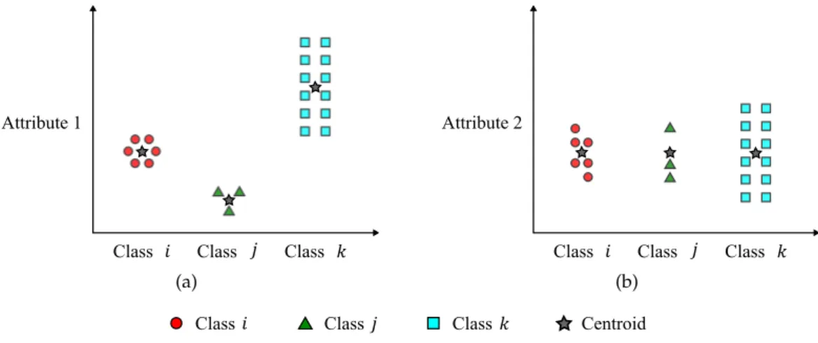
In order to assign weights to attributes, it is necessary to create an evaluation method for setting their discriminant power. We could say that the ideal attribute would present different average values for each class, but a constant value within each class. Figure

3.7 shows an example where attribute 1 can be considered discriminant but attribute 2 cannot. In fact, attribute 1 presents different centroid (average) values for each class, but similar centroid values for attribute 2. Besides, attribute 2 present higher dispersion values considering their centroid for classiand classj, than attribute 1. These two factors indicate the attribute 1 should be considered better than attribute 2.

(a) (b)

Figure 3.7: Different attribute set discriminant power example.

Thus, we value two factors in attributes: higher variances among class centroids and

(41)

3. IMPROVINGKNN – SOLUTIONS 3.2. Weighted Attributes

lower variance within each class regarding its elements.

We defineImportanceof an attribute (Equation3.1), in short, as being the quotient of how much the attribute value deviates through classes and how much it deviates inside each class. In other words, we can set the Importance as being the ratio between the variance of the average value of that attribute for each class (Equation3.2) and the average of the local variances (Equation 3.5). By local variances we mean the variance of the attribute value within each class, regarding its elements (Equation3.6).

Keeping this idea in mind, we can define the Importance of attribute a,Imp(a), by the expressions below presented.

Imp(a) = VM(a)

MV(a) (3.1)

VM(a) = 1

#Classes.

X

ci∈Centroids

(ci−c)2 (3.2)

c= 1

#Classes.

X

ci∈Centroids

ci (3.3)

ci=

1

#Elements in Classi

. X

e∈Classi

ve,a (3.4)

MV(a) = 1

#Classes.

X

ci∈Classes

LV(a, ci) (3.5)

LV(a, ci) =

1

#Elements in Classi

. X

e∈Classi

(ve,a−v.,a)2 (3.6)

v.,a=

1

#Elements in Classi

. X

e∈Classi

(ve,a) (3.7)

To calculate how much an attribute a deviates through classes we start by computing each class centroidc, this is, computing mean value for attribute a using class elementsve,a

as expressed by expression (Equation3.4). Having this result, the average centroid value is set asc, shown in expression (Equation3.3). Then, these values are used to determine how much those centroids deviate from their average value, and it is set asVM by expression (Equation3.2). As it was mentioned, the higher theVM(a)value the more important the attribute is, it will be placed as the dividend ofImp(a).

In expression (Equation3.6), each local variance,LV(a, ci)value uses all attributea

values of classcelements, represented asve,aabove and computes its mean value asv.,a

as in expression (Equation3.7). As lower local variances correspond to stronger attributes,

(42)

3. IMPROVINGKNN – SOLUTIONS 3.3. Converting Categorical Data to Continuous Data

3.3 Converting Categorical Data to Continuous Data

As mentioned earlier, continuous attributes such as ages, heights, weights, etc, allow precise measurements. Any data set of this data type can be placed in ascending or descending order. So, the distance/difference between two values can be highly accurate computed.

On the other hand, categorical data usually represents characteristics such as gender, blood type, marital status, etc. Despite categorical attributes may take numerical values, they may not represent mathematical values, for example categories codes or color rep-resentations, among others. Therefore there is no intuitive way to compute differences between two values from different categories of this data type. Typically, this problem is solved by setting this difference as 1 if values are different or 0 if they are the same. Not only does this method is not sensitive enough to accurately evaluate categories regarding their realdistances, but it also does not take into account the impact of the category values in terms of class distribution. Moreover, using categorical data on the data structures presented before would result in highly inaccurate classifications, once the approach we are using is highly dependent on the accuracy of distance measurements.

To address this problem, instead of adapting the structure in any way that would fit this data type, our approach involves transforming categorical data to numerical data. In other words, for each categorical attribute, we transform all possible values into numeric values. The major obstacle applying this method is that even if it was possible to assign distinct numeric values to each categorical value of a categorical attribute, it is even harder to set the displaying order.

Table 3.1: Eye color distribution over hemispheres.

Gender Eye Color Hemisphere

Male Blue North Male Green North Male Green North Male Green South Male Green South Male Dark North Male Dark South Female Blue North Female Blue North Female Green North Female Green North Female Green South Female Dark North Female Dark South Female Dark South

As an example, by Table3.1, apparently there is no obvious way to order the different

(43)

colors concerning the ability to discriminate both classes (North or South).

However, this table hides important information that can lead us to find such order. The transformation proposed in this thesis takes conditional probabilities as its base. Thus, if we consider the given example for the eye color attribute, we get the following conditional probabilities:

Table 3.2: Eye color conditional probabilities.

P(EyeColor|Hemispher) Eye Color South North

Blue 0 0.33

Green 0.5 0.44

Dark 0.5 0.22

Considering the South and North classes as being the edges of the interval [0,1]

respectively, it is possible to compare different eye color values. If we consider the blue eyes conditional probabilities (from Table3.2), even if it is known that only 33.3% of all individuals in the north hemisphere have blue eyes, we can conclude that any individual who has blue eyes is for surely from the north hemisphere. It is possible to make such affirmation due its representation in the overall world, due to its percentage: ₍₀₊₀0.33_.₃₃₎ = 1. This introduces a functionScaleCatdefined as:

ScaleCat(Cat, Classi, Classj) =

P(Cat|Classi)

P(Cat|Classi) +P(Cat|Classj)

where for example, Cat is "Blue" andClassiandClassj is "South" and "North". When

applying this function to all color eye attribute values we get:

ScaleCat(”Green”,”N orth”,”South) = P(”Green”|”N orth”)

P(”Green”|”N orth”) +P(”Green”|”South”) = 0.44

(0.44 + 0.5)

= 0.47

ScaleCat(”Dark”,”N orth”,”South”) = 0.22

(0.22 + 0.5)= 0.31

ScaleCat(”Blue”,”N orth”,”South”) = 0.33

(0.33 + 0) = 1

(44)

of "Blue" in that scale, only ScaleCat(”Green”,”South”,”N orth”) must be used; not

ScaleCat(”Green”,”N orth”,”South”).

This approach enables more thorough measurements since distances do not only take the two typical values (0 and 1 for different and equal classes respectively). Although it would be easy to say that individuals having blue eyes would be somehow more related with the north hemisphere, we were not able to quantify how much they would differ from dark and green eyes individuals. By this approach we transform data in such way we can even say that the difference between green and dark eyed individuals is smaller than either of them towards blue eyed individuals. In a general perspective, this means that we can generate an axis as show below in Figure3.8.

Figure 3.8: Eye color attribute transformation axis.

The same process must be applied to the other attribute and its categories, that is,

ScaleCat(”M ale”,”N orth”,”South”)andScaleCat(”F eale”,”N orth”,”South”)must be computed.

This method ables the comparison of categorical attributes values between any two classes. So in this particular example, the dataset which contains just two categorical attributes over two classes would be transformed into another dataset but containing two numerical attributes.

In a general way, any dataset containingAcategorical attributes overKclasses will be transformed into a new set containing K₂

×Anumerical attributes. This may end up in a large number of new attributes, as being the result of all combinations representing all possible pairs of classes. Apparently, this turns out to be the downside of this solution once increasing the number of attributes implies a greater computational weight in the learning phase. Despite that, it may happens that not all new attributes are meaningful once their implicitScaleCat(., ., .)values present no discriminant ability in the context of some pairs of classes. Thus, it is possible to use the previously presented attribute’s weights or PCA (Principal Component Analysis) to select and use only the more meaningful attributes.

In [CAdC11], theValue Difference Metricmeasures distances between pairs of categor-ical values. Although, by using it, it is not possible to sort those values in a numercategor-ical axis. The authors in [IPM09] also focus the problem of defining a distance between pairs of values of the same categorical attribute. They consider it to be a difficult task once those categorical values are not ordered. Instead of the learning-classification context, the au-thors try to obtain good clustering performance by using numerical instead of categorical data. The key intuition of their approach,DILCA, is that the distance between two values of a categorical attributeXcan be determined by the way in which the values of the other attributesY are distributed in the dataset objects: if they are similarly distributed in the groups of objects in correspondence of the distinct values ofXa low value of distance is

(45)

obtained. More specifically, it is a two-step method. In the first step, for each categorical attributeX, first a suitable context constituted by a set of attributesY 6=Xis identified, such that each attribute belonging to the context is correlated to the attributeX. In the second step, a distance matrix between any pair of values (xi,xj) ofXis computed: the

distribution ofxi andxj in objects having the same values for the context attributes is

(46)

(47)

4

Results

4.1 Dataset Collection

In order to test the developed tools, a collection of datasets were considered. Gathering datasets was somehow a subjective task since there were no evaluation methods to select them. Still, some characteristics were considered. The content of the considered datasets should be, if possible, meaningful or helpful to some purpose. Another important feature in this gathering was the number of classes in the dataset and having a reasonable balance between class distributions. Furthermore, in order to evaluate the tools proposed in this thesis, dataset should have a considerable number os attributes (at least three).

Restrictions on attribute’s quality were not applied, since feature correlation and low quality of the attributes is a reality and may be present in any dataset.

To test the developed tools, it was essential to have datasets based on numerical and categorical data. Considered datasets containing numerical data were:

• Iris (IRIS) dataset is one of the most popular dataset in pattern recognition. It describes 3 types of iris plant over 4 numerical features reflecting sepal and petal length/width. It has a perfect balanced class distribution, having 50 records for each of 3 classes;

(48)

4. RESULTS 4.1. Dataset Collection

• Auto-Mpg Data (AMPG) is an adapted dataset which aims to classify the origin of an automobile based on 4 numerical attributes: fuel consumption in mpg, engine displacement, engine horsepower and automobile’s total weight. In this dataset, the whole 392 automobiles can come from 3 continents: America, Europe or Asia, whose distributions are respectively 62.5%, 17.3% and 20.2%;

• Haberman’s Survival Data (Haberman) contains 306 cases from a study conducted between 1958 and 1970 at the University of Chicago’s Billings Hospital on the survival of patients who had undergone surgery for breast cancer. Each case is characterized by 4 numerical attributes: age of patient at time of operation, patient’s year of operation and number of nodes detected. Each case is classified into two classes which indicate if patient has survived or not within 5 year. In 73.5% of the cases, patients survived;

• Thyroid Disease (TD) is a study on hyperthyroidism regarding 215 subjects. Each subject is characterized through 5 numerical features regarding hyperthyroidism tests: T3 Resin, Thyroxine and Triiodothyronine hormones and 2 Thyroid-Stimulating Hormone tests. Hyperthyroidism is present in 16.3% of the subjects;

• Blood Transfusion Service Center Data Set (BT) contains information from a Blood Transfusion Service Center in Hsin-Chu City in Taiwan. This dataset was elaborated in order to build a FRMTC model and describes 748 donors at random from the donor database. Donators data consist on 4 numerical attributes: months since their last donation, number of donations, total blood donated in c.c. and the number of months since first donation. Individuals are separated in two classes, representing whether if he/she donated blood in March 2007. Having 2 classes, 23.8% of the individuals have donated at the specified month. The datasets based on categorical data were:

• Census-Income (Census) is also one of the most popular dataset in pattern recog-nition. It consists on an extraction done by Barry Becker from the 1994 Census database. From the 30725 samples considered in this dataset, about 24.9% are classi-fied as making over 50K a year. Each sample has categorical information relative to a person’s: age, work class, education, marital-status, relationship, race and gender;

• Car Evaluation Database (CED) contains information regarding automobile quality. It was derived from a simple hierarchical decision model originally developed for the demonstration of DEX (a system shell for decision support). This dataset contains 1728 examples with 6 categorical attributes: buying price, maintenance price, doors, passenger capacity, luggage boot size and safety. Automobiles can be classified in 4 quality classes: "unacceptable", "acceptable", "good" and "very good", whose distributions are respectively 70%, 22.2%, 4% and 3.8%;

(49)

4. RESULTS 4.2. Data Structures

• Nursery Dataset (Nursery) reflects a hierarchical decision model originally devel-oped to rank applications for nursery schools. It was used during several years in 1980’s when there was excessive enrollment to these schools in Ljubljana, Slovenia, and the rejected applications frequently needed an objective explanation. The 12960 subjects in dataset were evaluated based on several characteristics: parents’ occu-pation, child’s nursery, form of the family, number of children in family structure, housing conditions, financial standing of the family and family’s social and health conditions. Final classification may result in 5 possible evaluations which are dis-tributed in the following way: "not recommended" (33.33%), "recommended" (0.02 %), "very recommended" (2.53%), "priority" (32.91%) and "special priority" (31.21%);

• Wisconsin Breast Cancer Database (WBC) was obtained from the University of Wisconsin Hospitals, Madison from Dr. William H. Wolberg. Its data contains information about 699 individuals whose nodles had been tested for breast cancer. Each subject’s test is characterized over 9 features: clump thickness, uniformity of cell size (and shape), marginal adhesion, single epithelial cell size, bare nuclei, normal nucleoli and bland chromatin mitoses. Having 2 possible classes, 65.5% of subjects are classified as "benign";

• Contraceptive Method Choice (CMC) is a subset of the 1987 National Indonesia Contraceptive Prevalence Survey. The samples are married women who were either not pregnant or do not know if they were at the time of interview. Those interviews result in a dataset with 1473 samples over 9 categorical features: age, education, husband’s education, successful births, religion, employed (yes/no), husband’s occupation, "standard-of-living index", media exposure. Every interview results in a contraceptive usage class. These classes distributions are: "no use" (42.7% of the dataset), "long-term" (22.6%) or "short-term" (34.7%);

• Hayes-Roth & Hayes-Roth (Roth) dataset involves human subjects study containing 132 instances. It has information over 4 categorical attributes: hobby, age, educational level and marital status. This dataset includes 3 classes, which are distributed in the following proportions: 38.6%, 38.6% and 22.7%.

Table4.1summarizes dataset’s main characteristics.

4.2 Data Structures

4.2.1 Characterization of the Tests

Data structures were developed so that by introducing a learning phase, the classifica-tion of new objects would become faster. As important as reducing classificaclassifica-tion time, maintaining accuracy is imperative.

(50)

Table 4.1: Dataset collection features.

Name Data Type Samples Attributes Classes

IRIS Numerical 150 3 3

Vehicles Numerical 3100 4 3

AMPG Numerical 392 5 3

Haberman Numerical 306 4 2

TD Numerical 215 5 2

BT Numerical 748 4 2

Census Categorical 30725 7 2

CED Categorical 1728 6 4

Nursery Categorical 12960 8 5

WBC Categorical 699 9 2

CMC Categorical 1473 9 3

Roth Categorical 132 4 3

datasets were split 150 times into two disjoint subsets, the training set, containing 97% of the whole data, and test sets. Each time, one of these sets used the training set as the knowledge base and tried to classify the remaining samples (as new objects) in the test set resorting to all data structures. This way, in order to compare the performance of the different datasets, all datasets are processed using the same dataset split, considering severalKnearest neighbors (up to 13). This was repeated for the 150 splits.

Those same data set splits will be maintained for testing weighted attributes, which are described in Section 3.2. Furthermore, the same data splitting method is applied to categorical data for testing categorical-to-continuous data conversion in Section3.3. Original KNN and Fixed Grid structures performance values were used as reference.

Testing data structures also involves testing the following variants:

• Original KNN runs as expected, using euclidean distances. Its results will be used as basis for comparison for all developed data structures;

• Fixed Grid is a very straightforward structure as it does not include variants. As referred, it has disadvantages associated. However, as it was the starting point in developing other structures, its test results are relevant to follow up the structures enhancement process;

• QuadTree has 4 variants. The first variant interferes with the learning phase process, more specifically with each one of the two heuristics to be used, as it was detailed in the learning phase in Subsection3.1.2. The second one relies on a study about the impact of data normalization in the final outcome, which can be used or not;

• KD-Tree uses the exact same 4 variants as the QuadTree. This was considered due to these data structures similarity;

• InTree is analogous to QuadTree and KD-Tree in so many aspects that it makes sense to have the same variants to be tested.

(51)

4.2.2 The Most SuitableK

Somehow, the burden of choosing theKvalue in the classification process of the Original KNN algorithm may be seen as a consequence of its lazy-learning nature. Using the non-lazy-learning approach proposed on this thesis, it is possible to recommend aKvalue (or a short set ofKvalues) which were previously evaluated as being the most suitable one to get the best accuracy for each specific dataset.

Every time a data structure variant is tested on a dataset split (a run), the test set is classified 13 times, corresponding to the 13 consideredK values. The highest and lowest accuracy obtained from these tests are kept, and the highest one can be recommend the user. As we will see in next subsection (Subsection4.2.3), for each test combining a data structure variant and a dataset, terms%Hand%Lrepresent this extremes.

Lower extremes were not discarded from some tables and figures in order to show the influenceK value has in the accuracy for each case.

4.2.3 Results

The following graphics are the results from the 150 runs on each possible combination between datasets, data structures and its own variants. To interpret these results it is mandatory to understand that each graphic represents the tests over a data structure variant. Each data structure graphic contains pairs os columns. Each pair represents the highest and lowest accuracy results on average for the 150 runs for a dataset – by highest and lowest we mean the best and the worst suitableKnearest neighbor accuracy value –. Our reference accuracy values are also present an intervals. The interval between the highest and the lowest accuracy values (in average) for Original KNN data structure is represented by two black small horizontal lines. For the Fixed Grid, interval is represented by the two red lines also meaning highest and lowest accuracy.

As an example, let us take the case of Figure 4.7, which depics the accuracy value results for the QuadTree structure tests using normalized data and SDH heuristic over all datasets. Thus, taking the BT dataset pair of columns, the dark and light blue bars represent respectively the best and the worst accuracy considering the differentKvalues, for this QuadTree structure variant. The top and bottom black lines represent the best and the worst accuracy obtained for the considered set ofKvalues using the Original KNN. The top and bottom red lines have the same meaning but for the Fixed Grid.

In this particular example, we can conclude that for BT dataset, this QuadTree structure variant classifies new objects obtaining higher accuracy values than both Original KNN and Fixed Grid. As for the lowest accuracy values, while it has been beaten by the Original KNN, it is still better than the Fixed Grid.