A modified potential for HO
2with spectroscopic accuracy
João Brandão,1,a!Carolina M. A. Rio,1and Jonathan Tennyson2
1
Departamento Química Bioquímica e Farmácia, FCT, Universidade do Algarve, Campus de Gambelas, 8005-139 Faro, Portugal
2
Department of Physics and Astronomy, University College London, Gower Street, London WC1E 6BT, United Kingdom
sReceived 6 November 2008; accepted 24 February 2009; published online 3 April 2009d Seven ground state potential energy surfaces for the hydroperoxyl radical are compared. The potentials were determined from either high-quality ab initio calculations, fits to spectroscopic data, or a combination of the two approaches. Vibration-rotation calculations are performed on each potential and the results compared with experiment. None of the available potentials is entirely satisfactory although the best spectroscopic results are obtained using the Morse oscillator rigid
bender internal dynamics potential fBunker et al., J. Mol. Spectrosc. 155, 44 s1992dg. We present
modifications of the double many-body expansion IV potential of Pastrana et al.fJ. Chem. Phys. 94,
8093 s1990dg. These new potentials reproduce the observed vibrational levels and observed
vibrational levels and rotational constants, respectively, while preserving the good global properties
of the original potential. © 2009 American Institute of Physics.fDOI:10.1063/1.3103491g
I. INTRODUCTION
The hydroperoxyl radical HO2 is an important
interme-diate in combustion as well as playing a role in interstellar
chemistry. For this reason, and because HO2 represents an
intermediate in the reaction H + O2↔ O + OH, there have
been many studies of the potential energy surface of its
X ˜ 2
A9 ground state, see, for example, Refs.1–10and
refer-ences included in those articles.
As a result of these studies there are a variety of
poten-tials available for performing dynamical studies on HO2,
both in order to determine its rovibrational states and for modeling chemical reactions. Furthermore, in the commonly
used many-body expansionsMBEd approach to building
po-tential energy functions,11the potential of HO2represents an
important, but relatively poorly defined, component of the
potential of the important H2O2molecule. For this reason we
considered it worthwhile to undertake a systematic and
criti-cal survey of the potentials available for the HO2 radical.
Here we report the results of this study.
II. POTENTIAL ENERGY FUNCTIONS
Out of the published potentials which represent the
po-tential minimum sminimad on the X˜ 2A
9 ground electronic
state of HO2, we decided to test those potentials we consider
to be the most accurate and those which cover the different procedures used in their construction. The seven potentials
we choose4–10 include the most accurate and recent ones.
Below we consider them in turn, in order of date of publica-tion.
The MBE potential of Farantos et al.4uses a MBEsRef.
11d whose parameters have been fitted to reproduce the
ex-perimental geometry,12well depth,13and the harmonic force
field deduced from the experimental vibrational data of
Ogilvie.12 The MBE potential does not include any
correc-tion for anharmonicity effects.
The DMBE IV potential of Pastrana et al.5is a double
MBE potential.14It was mainly fitted to the ab initio points
of Walch et al.,15 semiempirically corrected using the
DMBE-scaled-external correlation method,16 augmented by
ab initio data from the work of Melius and Blint,17 and
Walch and Rohlfing.18The potential was forced to reproduce
the experimental equilibrium geometry,19 dissociation
energy,15 and quadratic force constants4,20 of the
hydroper-oxyl radical. Again the vibrational information was included using the harmonic force field.
The third potential is the Morse oscillator rigid bender
internal dynamicssMORBIDd function21,22due to Bunker et
al.6This potential was obtained by fitting the more recent ab
initio calculations of Walch and Duchovic,23 and further points computed at the request of Bunker et al. Four param-eters of the potential, so obtained, were adjusted using MOR-BID calculation to reproduce the four known vibrational
energies24,25 and associated rotational constants. The
MOR-BID method is approximate which has been shown to give results with an average overestimate of the band origins by
1.1 cm−1with a standard deviation of 6.4 cm−1 from those
calculated using an exact kinetic energy operator for the H2O
molecule.26 These errors are in turn reflected in potential
functions fitted by this way. However, Bunker et al.6checked
their MORBID results with an independent discrete variable
representationsDVRd based method. It should be noted that
our calculations reported below do not agree exactly with the
DVR calculations of Bunker et al.,6being in close agreement
sless than 0.5 cm−1d with their MORBID results. The main
discrepancies come from levels s100d and s200d where the
differences are 1.1 and 4.7 cm−1, respectively. Our
imple-mentation of the potential is precisely that given in the paper of Bunker et al. and, despite discussions with the authors, it
ad
Electronic mail: [email protected].
THE JOURNAL OF CHEMICAL PHYSICS 130, 134309s2009d
remains unclear what is the cause of this discrepancy. Fi-nally, the functional form used in this potential does not re-produce the symmetry needed to describe the exchange of the H atom between the two O atoms.
The Walch, Dateo, DuchovicsWDDd potential was
con-structed by Dateo7 using the same ab initio data of Walch
and Duchovic.23Although using a different functional form,
the WDD surface has two- and three-body terms, each with short- and long-range terms, in a similar fashion to the DMBE method.
A different diatomics-in-molecules27,28 sDIMd approach
was taken by Kendrick and Pack.8 Using the DIM model,
Kendrick and Pack were able to fit accurately a large set of
ab initiocalculations from Walch and co-workers.15,18,23,29,30 The DIM model is a multisurface approach and the DIM potential is able to correctly reproduce the conical
intersec-tions known to exist for HO2at C2vand collinear geometries.
All the other potentials used here are single valued surfaces which cannot reproduce these features. However, as pointed out by Kendrick and Pack, the diatomic potentials are based on Morse potentials and cannot accurately describe vibra-tionally excited states beyond the third vibrational level.
The next potential we use in this work is the DMBE
IV-S potential of Varandas et al.9These authors adjusted the
DMBE IV potential in order to reproduce the fundamental
frequencies of the H16O
2radical.
25,31
This was achieved us-ing rigorous vibrational calculations and a trial-and-error scaling of the internal coordinates. As noted by the authors, the scaling procedure they use slightly modifies the equilib-rium properties of the original DMBE IV potential energy surface, and hence introduces small errors in the rotational constants relative to the unscaled surface.
Recently, Guo and co-workers10,32,33 published a global
analytical potential based on a cubic-spline fit of 15 000
high-quality sDavidson corrected internally contracted
mul-tireference configuration interaction or icMRCI+ Qd ab initio
points with a largesaug-cc-pVQZd basis set, this new
poten-tial is denoted XXZLG PES. These authors comment that
their potential energy surface sPESd provided a much
im-proved agreement with experimental fundamental vibrational
frequencies with errors less than 10 cm−1as opposed to the
100 cm−1 found with the DMBE IV PES.10 Lin et al.34,35
also showed that the XXZLG PES gives much better agree-ment with the available spectroscopic data than the DMBE IV PES.
In summary, in this work we test potential energy sur-faces with different genesis. They range from the exclusive
use of the force field, MBE,4use of ab initio calculations and
force field, DMBE IV,5 mix of ab initio calculations and
MORBID vibrational calculations,6 only ab initio
calcula-tions fitted to a single valued function, WDD,7or to a DIM
model, DIM,8using rigorous vibrational calculations, DMBE
IV-S,9 and the XXZLG PES sRef. 10d that is based on a
cubic spline of about 15 000 ab initio points.
Of those potential energy surfaces, only the MORBID function of Bunker et al. does not aim to span all of configu-ration space. Designed for spectroscopic studies, this poten-tial does not reproduce the dissociation to diatomic frag-ments nor the internal isomerization of HOO into OOH, a
process which is known to be allowed at all collision ener-gies. All the other potentials are designed to reproduce the
main features of the HO2potential energy surface.
Recent developments on the multiphoton technique ca-pable of probing the vibration-rotation states of water just above and just below its dissociation limit with spectroscopic
accuracy, see Ref. 36, and on the dynamics of the
intramo-lecular energy transfer in the isotopic branching ratio on the
O + HD reaction37have shown the necessity of global
poten-tial energy surfaces, accurate for all the configuration space and useful for both spectroscopic and dynamic studies. This is a goal nowadays feasible for small polyatomic systems.
A comparison of the predictions for the location, depth,
and force field of the HO2 potential minimum is given in
TablesIandII. The last two rows of those tables refer to the
new potentials sDMBE IV-V and DMBE IV-VRd, proposed
in this work, see Sec. IV for details. We note that only the MBE and DMBE IV potentials, although using different sources, were explicitly fitted in order to reproduce the ex-perimental information available for the geometry, well depth, and force field. The MORBID, WDD, and DIM po-tentials used the ab initio energy values of Walch et al. as source data. The small differences we find in the predictions from those potentials came from the set of points used, the
TABLE I. Properties of the minimum and C2vsymmetry saddle point for the
HO2electronic ground states potential energy surfaces used in this work.
RO–O sa0d RO–H sa0d aOOH sdegd De a sEhd Minimum Empiricalb 2.5144s16d 1.8344s38d 104.29s31d 20.279 0 MBEc 2.570 1.861 106.0 20.274 66 DMBE IV 2.5143 1.8345 104.29 20.278 97 MORBID 2.5134 1.8358 104.31 ¯ WDD 2.5166 1.8357 103.84 20.267 55 DIM 2.524 1.839 100.61 20.274 07 DMBE IV-S 2.4930 1.8386 102.28 20.278 97 XXZLGd 2.521 1.836 104.12 20.273 69 DMBE IV-V 2.5143 1.8345 104.29 20.278 97 DMBE IV-VR 2.5263 1.8588 106.08 20.278 18 RO–O sa0d RO–H sa0d aOHO sdegd Ve sEhd Saddle point MBEc 2.422 2.205 66.63 0.066 8 DMBE IV 2.806 2.272 76.27 0.064 9 MORBID ¯ ¯ ¯ ¯ WDD 2.686 2.184 75.89 0.061 1 DIM 2.663 2.207 74.21 0.060 4 DMBE IV-S 2.758 2.256 75.36 0.064 9 XXZLGd 2.724 2.192 76.80 0.061 3 DMBE IV-V 2.802 2.270 76.22 0.065 3 DMBE IV-VR 2.802 2.271 76.20 0.064 6 a
Well depth energy relative to the three isolated atoms.
b
See Refs.15and19, values in parentheses represent estimated uncertain-ties.
c
This potential has used, as input data, the experimental values given in Refs.12and13.
d
See Ref.10.
e
functional form used, and from the quality of the fit. Note that the MORBID potential has been, in a second step, read-justed to reproduce observed spectroscopic data, and so, it has a slightly different harmonic force field. Comparing the properties of the DMBE IV and DMBE IV-S potentials, we can also see the effect of the scaling procedure used to adjust the DMBE IV-S potential.
It is interesting to note in Table II that the potentials
fitted to the ab initio data or the observed vibrational fre-quencies have larger values for the force constants, in
par-ticular, F11, F22, and Faa, when compared to the values
de-duced from experiment. This is particularly notable when comparing these values for the DMBE IV and DMBE IV-S potentials: the DMBE IV potential exactly reproduces the experimental force field, but the DMBE IV-S potential, which is a recalibration of the DMBE IV potential to repro-duce the observed vibrational spectra, does not.
Another important feature, when computing spectra of this radical, is the saddle point for the exchange of the H
atom between the two O atoms. In TableIwe also compare
the geometry and energy of this point on the different poten-tials. Bunker and co-workers pointed out that this feature
snear 13 000 cm−1d would not have a significant effect on
the low-lying vibrational energies. Note, however, that its position determines the difference between odd and even states for the vibrational wave function. Our calculations low found differences between the amount of splitting be-tween states which are odd and even with respect to the
interchange of O atoms, see Barclay et al.,38for example, for
the various potentials tested. For the highest states discussed
below our calculation found splittings of about 0.001 cm−1
between odd and even symmetry calculations. Splittings of this magnitude are probably not significant, especially when one considers that this and previous studies ignore any
ef-fects of spin on the rotational levels. Furthermore, for H16O
2
at least, this splitting cannot be determined experimentally, and for this reason we do not pursue this aspect of the prob-lem here.
It has been pointed out that the X˜ 2A9ground state of the
HO2radical correlates with a P state at collinear geometries
and, due to the degeneracy with the A˜ 2A8first excited state,
the Renner–Teller effect should be considered.39,40However,
the collinear saddle point of the DMBE IV potential lies
17100 cm−1above the bottom well, which is a high energy
when compared to those used in our calculations. We have computed the probability of finding the system in configura-tions close to the collinear geometry,
E
0aS
E
0`E
0`C2su,r,RddrdR
D
du.When using the wave function ofs200d level for the DMBE
IV potential, we find the probabilities to be 1.13 10−4, 3.8
3 10−7, and 1.33 10−10fora= 30°,a= 20°, and a= 10°,
re-spectively. We found lower values for the other levels. This results show that this probability fast decreases to zero as the system approaches collinearity and, similar to other
calcula-tions in the same systems,9,35the Renner–Teller effect can be
neglected in this work.
Finally it should be noted that the low-lying excited
electronic state, A˜ 2A8, lies 7029 cm−1 above the ground
state24 and can thus be expected to perturb excited levels
associated with the ground state. This should particularly be borne in mind when considering the highest observed
vibra-tional band of the ground state, the s200d band, which is
known experimentally to be perturbed.24,41Indeed in
discuss-ing their observations, Fink and Ramsay42appeared to doubt
even the correctness of this assignment.
In their observational paper, Fink and Ramsay42
con-cluded with a plea for better data on the vibrational levels of
the ground potential energy surface at about 7000 cm−1 in
order to identify the perturbed they identified in their spectra. We have analyzed the results of the calculations on each the potentials discussed above and find that none satisfy the cri-teria of Fink and Ramsay in terms of vibrational band origin and rotational constants.
The interaction between these two electronic states has
been subject of accurate studies by Jensen and
co-workers.39,43,44Using ab initio calculations on both states,
these authors characterized the Renner–Teller effects at col-linear geometries and the spin-orbit interaction between the
X
˜ s112d vibronic state and the J,51/2 rotational levels of
the A˜ s000d state located at 7030 cm−1. With reference to
interaction between rovibrational states of the ground and
TABLE II. Force constants for the HO2electronic ground state potential energy surfaces used in this work.
F11 sEha0 −2 d F22 sEha0 −2 d Faa sEhd F12 sEha0 −2 d F1a sEha0 −1 d F2a sEha0 −1 d Expt.a 0.3774 0.4286 0.2211 ¯ 0.0414 ¯ MBEb 0.370 0.409 0.252 0.0093 0.0520 20.0549 DMBE IV 0.377 0.429 0.221 0.0063 0.0414 20.0621 MORBID 0.415 0.482 0.239 0.0161 0.0798 20.0118 WDD 0.459 0.504 0.239 0.0142 0.0941 20.0109 DIM 0.438 0.509 0.248 0.0189 0.0642 20.0185 DMBE IV-S 0.401 0.455 0.258 20.0156 0.0376 20.0740 XXZLG 0.412 0.476 0.234 0.0140 0.0831 20.0098 DMBE IV-V 0.420 0.468 0.271 20.0426 0.0265 20.0401 DMBE IV-VR 0.431 0.476 0.268 0.0104 0.0104 0.0168
aFitted values neglecting the effect of the anharmonicity, see Ref.20. b
This potential used a refinement by Mills and Carter of the force field given in Ref.12.
excited PESs, they comment that “at 7034 cm−1, however,
the A˜ 2A8 rovibronic states emerge and interaction becomes
more likely.”44 Furthermore, no such interaction between
these two states has been observed in the
6603.2– 6685.5 cm−1 region used to assign the 2n
1 band
constants45 used in this work. As a consequence no
off-diagonal electronic interactions are considered here when
computing the rovibrational energies for the X˜ s200dN=0 or 1
states.
III. ROTATION-VIBRATION CALCULATIONS
Calculations were performed using theDVR3D program
suite46in atom-diatom scattering coordinates which represent
the O2 as a diatomic with H as the atom. These coordinates
are natural for the HO2molecule, but it should be noted that
they automatically treat both symmetry-related minima in a nuclear motion calculation. This is a point discussed further below.
In our final calculations, the angular motions were
rep-resented using 40 grid points based onsassociatedd Legendre
polynomials. Grids for both the O2stretch and H – O2stretch
were based on the zeros of Morse oscillatorlike functions46
which are associated Laguerre polynomials. These functions
were characterized by parameter sets sre, De, wed sRef. 46d
equal, in atomic units, to s2.514,0.272 93,0.005 1204d and
s2.467,0.102 89,0.013 2207d, respectively. The final
calcula-tion used a grid of 28 points for the O2stretch and 20 points
for the H – O2 stretch. For N = 0 calculations, a final
Hamil-tonian of dimension 3100 was diagonalized. For N = 1 it was found that, in the second step of the calculation, a
Hamil-tonian of dimension 1000 was required to give converged
results for the C rotational constant of thes200d state.
Extensive tests were performed to check the conver-gence of our rotation-vibration calculations. In particular, it was found necessary to perform quite large calculations for
some potentials to obtain reliable results for thes200d
vibra-tional state. This state varied between numbers 28 and 31 in our J = 0 even calculations depending on which potential en-ergy surface was used. In some cases the state shows heavy mixing with other vibrational modes. For each potential we
assigned the s200d state on the basis of energy differences
and expectation values for the radial O–O and H–OO dis-tances. The OH stretching overtone should have a large
kRH–OOl value as well as a small value for kRO–Ol. For the
MBE, WDD, and DIM potentials, this method was
unam-biguous and allows us to assign it to the 31 sMBEd or 28
sWDD, DIM and XXZLGd levels. For the DMBE IV and DMBE IV-S potentials, we have been able to assign the level
31 to this state but, like Varandas et al.,9 we found some
mixing with level 30 that can be assigned to states103d. The
coupling between two states, levels 29 and 30, is most evi-dent for the MORBID potential which showed a particularly heavy mixing. As Bunker et al. fitted their potential to level 29, we chose to quote our results for this level. However, it should be noted that experimentally the assignment relies more heavily on transition intensity considerations which we have not tested in this work. Our final calculations are
con-verged to within 0.1 cm−1for thes200d state and much
bet-ter than this for the lower vibrational bet-term values. Within these error bars, our results agree with other accurate pub-lished results for these potentials.
TABLE III. Experimental values for vibrational energies and for rotational constantssA, B, Cd, in cm−1, the
number in parentheses is one standard error in units of the last quoted digits.
Evib A B C Ref. s000d 20.356 523 8s19d 1.118 034 0s17d 1.056 319 2s17d 59 s001d 1097.6258s1d 20.309 080s50d 1.105 532s37d 1.042 649s38d 31 s010d 1391.7540s2d 20.957 46s67d 1.116 40s180d 1.050 08s183d 60 s100d 3436.1951s4d 19.584 15s67d 1.122 41s40d 1.058 25s37d 25 s200d 6651.1876s38d 18.903 3s17d 1.122 3s38d 1.050 8s21d 45
TABLE IV. Calculated vibrational term values, in cm−1, for the potentials used in this work.
s001d s010d s100d s200d sviba Expt.b 1097.63 1391.75 3436.20 6651.19 MBE 1075.54 1136.96 2871.77 5385.09 704.80 DMBE IV 1065.50 1296.40 3333.73 6492.37 107.06 MORBID 1097.47 1391.75 3436.49 6646.24c 2.48 WDD 1139.49 1413.75 3516.53 6783.33 80.86 DIM 1149.29 1410.30 3524.02 6794.63 88.46 DMBE IV-S 1097.83 1392.03 3436.59 6687.62 18.22 XXZLG 1089.97 1388.77 3433.09 6633.97 9.67 DMBE IV-V 1097.63 1391.75 3436.20 6651.19 0.00 DMBE IV-VR 1097.63 1391.75 3436.20 6651.19 0.00 as vib=
Î
s1 / Ndoi=1 4 sx i exp− x i cald2, where xiare the vibrational energies.
b
See all figures and errors on TableIII. For more detail see Refs.25,31,45, and60.
c
The role of nuclear spin statistics in the levels of H16O2
has been the subject of some debate.47However, only states
represented by even angular grid are spectroscopically ob-servable and we only present results for these. This is in
contrast to some other studies,48–52which have instead
pre-sented results only for the odd states.
Next, we compare our results with the experimental data
quoted in TableIIIalong with their quoted uncertainties.
Table IV compares the various vibrational term values
computed in this work with the available experimental data. The MBE potential performs particularly poorly for the
s100d H – O2stretching fundamental. The ab initio WDD
po-tential is also 90 cm−1 in error for this mode and 50 cm−1
too high for thes001d bending fundamental. Perhaps not
sur-prisedly, the two potentials which give the best estimates for the fundamentals are those which used these data directly in fitting: the MORBID and DMBE IV-S potentials. Comparing with these potentials, the ab initio XXZLG potential agrees better with experiment than the DMBE IV-S potential only
for thes200d H – O2stretching overtone. Conversely the
po-tentials which used harmonic data do not give a satisfactory representation of vibrational fundamentals.
Following Bunker et al.6and others, we assess the
rota-tional data against experimentally determined rotarota-tional
con-stants. From ourDVR3Dbased procedure we used two ways
of determining these constants. The first is by performing
N= 1 calculations and using the three rotational term values
so determined to define the constants. This method assumes that centrifugal distortion effects are negligible for N = 1 and that none of the N = 1 levels in question are perturbed. For each state we calculate the three rotational energies for N
= 1 sk = −1 , 0 , 1d, then we obtain the rotational constants sA,
B, and Cd using the following equations:
A= 0.5 3sE10+ E11− E1−1d,
B= E11− A,
C= E10− A. s1d
The second method is to explicitly use the N = 0 wave func-tions to give vibrational averages for the appropriate
instan-taneous, inverse inertia tensor using the programXPECT3of
theDVR3Dsuite.46We have compared these two approaches
for all the potentials considered, and TableVsummarizes the
results obtained for the DIM potential which can be regarded as typical. The level of agreement between the two ap-proaches is generally very good, even for the rotational
con-stants ofs200d. Below we consider only results obtained
us-ing expectation values as the constants computed from our
N= 1 calculations proved rather sensitive to convergence of
this calculation.
Table VI compares rotational constants obtained by us
for all five vibrational states for which the corresponding constants have been experimentally determined. The DMBE IV and WDD potentials perform notably well for these con-stants, in contrast to their ability to reproduce the vibrational data. This is undoubtedly due to the accuracy with which these potentials reproduce the observed equilibrium structure
ssee TableId. Of the empirically determined potentials, only
the MORBID potential, which is based about the correct equilibrium geometry, gives satisfactory rotational constants. Similar results have been found for the XXZLG ab initio
TABLE V. Comparison, for the DIM potentialsRef.8d, between rotational constants, given in cm−1, computed
using expectation values or from energy levels, see Ref.61.
State
From expectation values From energy levels
A B C A B C s000d 19.75 1.113 1.053 19.74 1.117 1.053 s001d 19.71 1.099 1.039 19.70 1.103 1.039 s010d 20.37 1.107 1.048 20.36 1.117 1.049 s100d 19.02 1.115 1.049 19.02 1.119 1.053 s200d 18.32 1.115 1.045 18.31 1.122 1.052
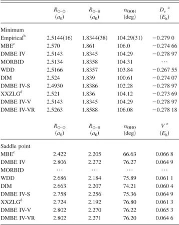
FIG. 1. Contour plot for the DMBE IV-VR potential for an O atom moving around an equilibrium OH diatomic with the center of the bond fixed at the origin. Contours are equally spaced by 0.01 Eh, starting at −0.277 Eh.
potential which also presents an equilibrium geometry close to experiment.
Most notably, the DMBE IV-S behaves poorly for the rotational constants. This potential, which gave excellent re-sults for the vibrational fundamentals, is a scaled version of the DMBE IV potential which gives good results for the rotational constants. However, the method of scaling used is to adjust the geometric parameters to improve the estimates
of the vibrational levels.9 Such a procedure has been
em-ployed by Bowman and Gazdy53,54for other triatomic
mol-ecules.
The importance of the true potential of a molecule giv-ing a reliable representation of both the vibrational and rota-tional levels of the molecule has been discussed at length
elsewhere.55 It would appear that the internal coordinate
scaling procedure applied to the DMBE IV-S potential is bound by construction not to achieve this result. This raises serious concerns about what such potentials represent and hence the method used for their construction.
IV. MODIFIED DMBE IV-V AND VR POTENTIALS
Due to the high quality of the dynamical results obtained using the DMBE IV potential, we improve its spectroscopic properties by adding a small term to modify the bottom well,
while retaining the overall behavior of the PES in those re-gions that should play an important role in controlling the reaction dynamics in this system. The functional form used for this extra term is a polynomial multiplied by a quadratic exponential term in the displacement coordinates from the equilibrium geometry. To ensure the permutation symmetry
of this system, we follow Schmelzer and Murrell56 and
de-fine coordinates invariant to the exchange of the two oxygen
atoms, i.e., the exchange of the R2 and R3 interatomic
dis-tances. Hence, the integrity basis is R1, S1= R2+ R3 and S2
=sR2− R3d2. Due to the existence of two symmetric minima
in this system, we use as displacement coordinates,
R1d= R1− R1eq, S1d= 1
Î
2fsR2+ R3d − sR2eq+ R3eqdg, s2d S2d= 1 2fsR2− R3d2−sR2eq− R3eqd2g,where the values for R1eq, R2eq, and R3eqare the quoted
ex-perimental equilibrium geometry1 2.5143a0, 1.8346a0, and
3.4592a0, respectively. These coordinates are simpler than
those used in the DMBE IV PES and are all zero at the two equivalent reference geometries.
TABLE VI. Rotational constants, in cm−1, calculated for the potentials used in this work.
s000d s001d s010d s100d s200d srota A 20.357 20.309 20.957 19.584 18.903 Expt.b B 1.118 1.106 1.116 1.122 1.122 C 1.056 1.043 1.050 1.058 1.051 A 20.43 20.43 21.92 29.04 485.89 MBE B 1.062 1.051 1.048 1.036 1.006 120.60 C 1.008 0.997 0.997 0.990 0.974 A 20.46 20.21 21.25 19.68 18.95 DMBE IV B 1.118 1.094 1.119 1.125 1.117 0.089 C 1.058 1.036 1.062 1.061 1.049 A 20.55 20.50 21.16 19.81 19.48 MORBID B 1.115 1.101 1.108 1.120 1.089 0.183 C 1.056 1.043 1.050 1.056 1.026 A 20.50 20.46 21.18 19.76 19.36 WDD B 1.113 1.098 1.105 1.118 1.105 0.149 C 1.054 1.040 1.047 1.055 1.040 A 19.75 19.71 20.37 19.02 18.32 DIM B 1.113 1.099 1.107 1.115 1.115 0.340 C 1.053 1.039 1.048 1.049 1.045 A 19.89 19.70 20.57 19.06 18.69 DMBE IV-S B 1.143 1.119 1.142 1.151 1.130 0.266 C 1.079 1.057 1.081 1.082 1.060 A 20.526 20.489 21.146 19.785 19.429 XXZLG B 1.109 1.095 1.101 1.113 1.087 0.167 C 1.050 1.038 1.044 1.050 1.025 A 20.47 20.31 21.17 19.61 18.87 DMBE IV-V B 1.118 1.101 1.115 1.123 1.109 0.063 C 1.058 1.043 1.057 1.059 1.042 A 20.36 20.31 20.95 19.58 18.90 DMBE IV-VR B 1.114 1.106 1.118 1.126 1.118 0.0024 C 1.053 1.043 1.050 1.060 1.055 as rot=
Î
s1 / Ndoi=1 15sx i exp− x i cald2, where xiare the rotational constants.
b
The functional form adopted for this additional term is a
third degree polynomials13 freely adjustable coefficients cid
multiplied by a decay term with four fixed terms ci fixsi
= 1 , 2 , 3 , 4d, T= c1+ c2R1d+ c3S1d+ c4R1d 2 + c 5S1d 2 + c 6R1dS1d+ c7S2d + c8R1d 3 + c9R1dS1d 2 + c10R1d 2 S1d+ c11R1dS2d+ c12S1d 3 + c13S1dS2d, DEC = c1fixR1d 2 + c2fixS1d 2 + c3fixR1dS1d+ c4fixS2d 2 , s3d
VRspect= T exps− DECd.
To achieve the accuracy of 0.01 cm−1 necessary to fit
the s200d state rotational constants, we changed to 80 grid
points for the angular motions, 60 grid points for the O2
stretch, and 40 grid points for the H – O2 stretch, instead of
the above referred 40, 28, 20 grid points used in theDVR3D
integration.
The derivatives of the vibrational energies with respect to the coefficients were computed using the Hellmann–
Feynman theorem,57 ]En ]ci =
E
Cnp]Hˆ ]ci Cndt=E
Cnp]VRspect ]ci Cndt. s4dThe necessary integrals were evaluated using the package
XPECT3of the DVR3Dsuite46 and the computed wave func-tions. The nonlinear fitting procedure was accomplished
us-ing the Marquardt algorithm.58
In a first step, we started fitting the four vibrational
en-ergies using only quadratic terms in Eq.s3d, but with c7S2d
2 to
guarantee values of zero for the first derivatives at the equi-librium geometry, and in this way keep the same geometry, i.e., T= c4R1d 2 + c5S1d 2 + c6R1dS1d+ c7S2d 2 . s5d
In this step we found that a constant value of 2.0 for the four
fixed terms ci fixsi = 1 , 2 , 3 , 4d in DEC was sufficient to yield
an exact fit to the vibrational levels with minor changes in the rotational constants of the DMBE IV PES and confine this term to the region of the bottom well. We call this
po-tential DMBE IV-Vsand the reduced additional term, Vspectd,
where V stands for vibration only. As shown in TableVIthis
potential slightly improves the rotational constants.
In a second step, starting from this potential, we add three linear and six cubic terms to fit the rotational constants. Derivatives of the rotational constants were computed using the derivatives of the three rotational term values given by
Eq.s1d. To combine the vibrational and rotational constants
in a same fit, we weigh the vibrational levels by 1.0, the A rotational constants by 10.0, and the B and C rotational con-stants by 100.0. The final potential, DMBE IV-VR, from vibration and rotation, still reproduces the vibrational
ener-gies with errors less than 0.005 cm−1 ssee Table IVd and
closely approaches the rotational constants with errors less
than 0.0022, 0.0038, and 0.0042 cm−1, for A, B, and C,
re-spectivelyssee TableVId. The fitted coefficients scid obtained
on the modified DMBE IV potentials are summarized on
TableVII.
V. GENERAL OVERVIEW OF THE DMBE IV-V AND VR POTENTIALS
The general properties of these new DMBE IV-V and
VR potentials are quoted in TablesIandIIto compare with
the other studied potentials. Comparing with the original DMBE IV potential, there we can see that both PESs display
similar geometry for the C2v saddle point, but while the
DMBE IV-V potential has the same minimum geometry and energy, the DMBE IV-VR potential shows small changes on its position and energy. This result contrasts with previous findings linking the minimum position with the rotational constants, see comment on the DMBE IV-S potential in Sec.
III and TableI.
Figure1shows a contour plot of the DMBE IV-VR PES
for an O atom moving around an equilibrium OH molecule. This picture is similar to that of the original DMBE IV
potential.5 A perspective view for the VRspect term is
pre-sented in Fig.2for the same geometries.
Another interesting view of those surfaces is shown in
Figs.3 and4where we plot the H atom moving around an
equilibrium O2molecule. Figure3displays a contour plot for
the additional term VRspectand a close view of this term near
the minimum geometry. There we can see that the main
con-tribution is on the stretching of the OH bonding. In Fig.4sad
we present the DMBE IV-VR and a close view of the bottom
TABLE VII. Fitted coefficients, in a.u., for the DMBE IV-V and VR poten-tials. Vspect VRspect c1 ¯ 1.094 421 9 3 10−3 c2 ¯ 2.938 960 3 3 10−4 c3 ¯ −9.472 370 5 3 10−3 c4 4.237 461 6 3 10−2 7.145 913 3 3 10−2 c5 1.286 578 6 3 10−2 2.298 432 1 3 10−2 c6 −5.257 641 3 3 10−2 −4.832 550 4 3 10−2 c7 3.237 781 8 3 10−3a 4.723 445 0 3 10−4 c8 ¯ −5.977 740 9 3 10−2 c9 ¯ 1.812 823 9 3 10−2 c10 ¯ 6.418 464 3 3 10−2 c11 ¯ −1.138 416 1 3 10−2 c12 ¯ 1.261 962 8 3 10−3 c13 ¯ −2.902 956 3 3 10−3 a
The coefficient c7is multiplied by S2d 2
, in the function T, see Eq.s3d.
FIG. 2. Perspective view for the additional term VRspectfor the same
geom-etries as Fig.1.
well, for comparison we also display the original DMBE IV
PES, see Fig.4sbd. We can see that both potentials have the
same general features, but there are noticeable differences in the bottom well, see contours A and B.
VI. CONCLUSIONS
We have tested seven potential energy surfaces
con-structed for the ground state of HO2. It would appear that
none of the potentials are entirely satisfactory.
The MORBID potential of Bunker et al.6gives the best
representation of the spectroscopic data but does not disso-ciate correctly. Indeed this potential does not represent the barrier between the two symmetry-related minima correctly,
a feature one would expect to influence the spectroscopy of the system at energies where tunneling splittings become sig-nificant.
The DMBE IV potential of Pastrana et al.5represents the
global features of the HO2surface and gives satisfactory
ro-tational constants. However, vibrational frequencies pre-dicted using it are considerably in error. The discrepancies found with this potential clearly indicate the that force fields are bad input data for calibrating the potential energy
sur-face. An attempt to rectify this problem by Varandas et al.9
produced the DMBE IV-S potential which does indeed give good results for the known vibrational term values, but only at the expense of the rotational structure of the problem.
The most recent potential made by Guo and co-workers
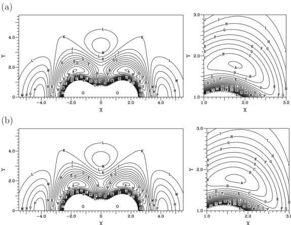
FIG. 3. Contour plot for the additional term VRspectfor a H atom moving around an equilibrium O2molecule with the center of the bond fixed at the origin,
at the right a close view of this term near the minimum geometry. Contours are equally spaced by 0.0005 Eh, starting at −0.001 Eh.
(a)
(b)
FIG. 4. Contour plot for a H atom moving around an equilibrium O2molecule with the bond center fixed at the origin, at the right a close view of this term
near the minimum geometry. Contours are equally spaced by 0.01 Eh, starting at −0.277 Eh.sad for the DMBE IV-VR PES and sbd for the original DMBE
gives reasonable good results for the known vibrational term values, but the rotational structure obtained is worse than the DMBE IV and similar to the WDD and MORBID potentials.
With a small additional Vspectterm, we have been able to
correct the bottom well of the DMBE IV potential. The new DMBE IV-V PES accurately reproduces the vibrational lev-els giving slightly better rotational constants than those of the original DMBE IV potential. Using 13 terms in the
ad-ditional VRspect term, we also have been capable to fit the
rotational constants. The new DMBE IV-VR PES accurately
reproduces the vibrational levels serrors ,0.005 cm−1d and
the rotational constants sroot-mean-square deviation srot
= 0.0024 cm−1d. While the DMBE IV-V PES conserves the
equilibrium geometry and energy of the DMBE IV potential, the DMBE IV-VR potential gives small changes for this ge-ometry and energy. Both potentials retain the remaining fea-tures of the DMBE IV PES; this is important as these play an important role in reaction dynamics on this surface for which
the DMBE IV potential is known to perform well.5
ACKNOWLEDGMENTS
We thank the referees for helpful comments. This work was supported by the FCT and the British Council under Grant No. LIS/882 and by FCT under the PTDC/CTE-ATM/ 66291/2006 research project.
1
M. J. Bronikowski, R. Zhang, D. J. Rakestraw, and R. N. Zare,Chem. Phys. Lett. 156, 7s1989d.
2
A. Viel, C. Leforestier, and W. H. Miller, J. Chem. Phys. 108, 3489
s1998d.
3
J. Troe and V. G. Ushakov,J. Chem. Phys. 115, 3621s2001d.
4
S. Farantos, E. C. Leisegang, J. N. Murrell, K. Sorbie, J. J. C. Teixeira-Dias, and A. J. C. Varandas,Mol. Phys. 34, 947s1977d.
5
M. R. Pastrana, L. A. M. Quintales, J. Brandão, and A. J. C. Varandas,J. Phys. Chem. 94, 8073s1990d.
6
P. R. Bunker, I. P. Hamilton, and P. Jensen,J. Mol. Spectrosc. 155, 44
s1992d.
7
C. E. Dateo,sunpublishedd, see Ref. 38.
8
B. Kendrick and R. T. Pack,J. Chem. Phys. 102, 1994s1995d.
9
A. J. C. Varandas, J. M. Bowman, and B. Gazdy,Chem. Phys. Lett. 233,
405s1995d.
10
C. Xu, D. Xie, D. H. Zhang, S. Y. Lin, and H. Guo,J. Chem. Phys. 122,
244305s2005d.
11J. N. Murrell, S. Carter, S. C. Farantos, P. Huxley, and A. J. C. Varandas,
Molecular Potential Energy FunctionssWiley, Chichester, 1984d.
12
J. F. Ogilvie, Can. J. Spectrosc. 19, 171s1973d.
13
S. N. Foner and R. L. Hudson,J. Chem. Phys. 36, 2681s1962d.
14
A. J. C. Varandas,Mol. Phys. 53, 1303s1984d.
15
S. P. Walch, C. M. Rohlfing, C. F. Melius, and C. W. Bauschlicher, Jr.,J. Chem. Phys. 88, 6273s1988d.
16
A. J. C. Varandas,J. Chem. Phys. 90, 4379s1989d.
17
C. F. Melius and R. J. Blint,Chem. Phys. Lett. 64, 183s1979d.
18
S. P. Walch and C. M. Rohlfing,J. Chem. Phys. 91, 2373s1989d.
19
K. G. Lubic, T. Amano, H. Uehara, K. Kawaguchi, and E. Hirota, J. Chem. Phys. 81, 4826s1984d.
20
H. Uehara, K. Kawaguchi, and E. Hirota, J. Chem. Phys. 83, 5479
s1985d.
21
P. Jensen,J. Mol. Spectrosc. 128, 478s1988d.
22
P. Jensen,J. Chem. Soc., Faraday Trans. 2 84, 1315s1988d.
23
S. P. Walch and R. J. Duchovic,J. Chem. Phys. 94, 7068s1991d.
24
R. P. Tuckett, P. A. Freedman, and W. J. Jones, Mol. Phys. 37, 379
s1979d.
25
C. Yamada, Y. Endo, and E. Hirota,J. Chem. Phys. 78, 4379s1983d.
26
J. A. Fernley, S. Miller, and J. Tennyson,J. Mol. Spectrosc. 150, 597
s1991d.
27
J. C. Tully, in Semiempirical Methods of Electronic Structure Calcula-tion, edited by G. SegalsPlenum, New York, 1977d, p. 173.
28
P. J. Kuntz, in Atom-Molecule Collision Theory, edited by R. B. Bernstein sPlenum, New York, 1979d, p. 79.
29
S. P. Walch and R. J. Duchovic,J. Chem. Phys. 96, 4050s1992d.
30
S. P. Walch,sunpublishedd, see Ref. 8.
31
A. R. W. McKellar, J. Chem. Soc., Faraday Discuss. 71, 63s1981d.
32
S. Y. Lin, H. Guo, P. Honvault, and D. Xie,J. Phys. Chem. B110, 23641
s2006d.
33
D. Xie, C. Xu, T.-S. Ho, H. Rabitz, G. Lendvay, S. Lin, and H. Guo,J. Chem. Phys. 126, 074315s2007d.
34
S. Y. Lin, H. Guo, P. Honvault, C. Xu, and D. Xie,J. Chem. Phys. 128,
014303s2008d.
35
C. Xu, B. Jiang, D. Xie, S. C. Farantos, S. Y. Lin, and H. Guo,J. Phys. Chem. A 111, 10353s2007d.
36
L. L. Lodi, O. L. Polyansky and J. Tennyson,Mol. Phys. 106, 1267
s2008d.
37C. M. A. Rio and J. Brandão, Chem. Phys. Lett. 433, 268
s2007d.
38
V. J. Barclay, C. E. Dateo, and I. P. Hamilton,J. Chem. Phys.101, 6766
s1994d.
39
G. Osmann, P. R. Bunker, P. Jensen, R. J. Buenker, J.-P. Gu, and G. Hirsch,J. Mol. Spectrosc. 197, 262s1999d.
40
P. Jensen, G. Osmann, and P. R. Bunker, in Computational Molecular Spectroscopy, edited by P. Jensen and P. R. BunkersWiley, New York, 2000d, Chap. 15, p. 485.
41
R. P. Tuckett, P. A. Freedman, and W. J. Jones, Mol. Phys. 37, 403
s1979d.
42
E. H. Fink and D. A. Ramsay,J. Mol. Spectrosc. 185, 304s1997d.
43
P. Jensen, R. J. Buenker, J.-P. Gu, G. Osmann, and P. Bunker,Can. J. Phys.79, 641s2001d.
44
V. V. Melnikov, T. E. Odaka, P. Jensen, and T. Hirano,J. Chem. Phys. 128, 114316s2008d.
45
J. D. DeSain, A. D. Ho, and C. A. Taatjes,J. Mol. Spectrosc. 219, 163
s2003d.
46
J. Tennyson, J. R. Henderson, and N. G. Fulton,Comput. Phys. Commun. 86, 175s1995d.
47
V. J. Barclay, C. E. Dateo, I. P. Hamilton, B. Kendrick, R. T. Pack, and D. W. Schwenke,J. Chem. Phys. 103, 3864s1995d.
48
X. T. Wu and E. F. Hayes,J. Chem. Phys. 107, 2705s1997d.
49
D. H. Zhang and J. Z. H. Zhang,J. Chem. Phys. 101, 3671s1994d.
50
V. A. Mandelshtam, T. P. Grozdanov, and H. S. Taylor,J. Chem. Phys. 103, 10074s1995d.
51
J. Dai and J. Z. H. Zhang,J. Chem. Phys. 104, 3664s1996d.
52
R. Chen and H. Guo,Chem. Phys. Lett. 277, 191s1997d.
53
J. M. Bowman and B. Gazdy,J. Chem. Phys. 94, 816s1991d.
54
B. Gazdy and J. M. Bowman,J. Chem. Phys. 95, 6309s1991d.
55
J. H. Schryber, O. L. Polyansky, P. Jensen, and J. Tennyson,J. Mol. Spectrosc. 185, 234s1997d.
56
A. Schmelzer and J. N. Murrell, Int. J. Quantum Chem. XXVIII, 287 s1985d.
57
R. P. Feynman,Phys. Rev. 56, 340s1939d.
58
D. W. Marquardt,J. Soc. Ind. Appl. Math. 11, 431s1963d.
59
A. Charo and F. C. de Lucia,J. Mol. Spectrosc. 94, 426s1982d.
60
K. Nagai, Y. Endo, and E. Hirota,J. Mol. Spectrosc. 89, 520s1981d.
61
J. Tennyson, Computational Molecular SpectroscopysWiley, New York, 2000d, Chap. 9, p. 316.
62
K. V. Chance, K. Park, K. M. Evenson, L. R. Zink, F. Stroh, E. H. Fink, and D. A. Ramsay,J. Mol. Spectrosc. 183, 418s1997d.